Nitin Kumar Mishra | Ranu*
© 2022 IIETA. This article is published by IIETA and is licensed under the CC BY 4.0 license (http://creativecommons.org/licenses/by/4.0/).
OPEN ACCESS
Emissions are a major contributor to climate change. Some nations are now concentrating their efforts on lowering carbon emissions. In many nations, carbon taxes and caps are the main tools that are used to attain this goal. The majority of the inventory retailer-supplier model assumed that the retailer’s order cost should be paid to the supplier at that time when he gets their order. Few suppliers can expect to receive the entire or a portion of the total cost in advance from retailers in this real-life situation, and others will offer prepayment in numerous equal installments. The advance payment offers the customer the lowest price for the order, but it has the largest carbon footprint. The advance payment has a great impact on carbon emissions and production. Therefore, this study looked at a carbon tax and cap supply chain inventory model for deterioration with carbon emission-dependent demand, and Three payment options: Preliminary, cash, and post-payment have been considered. The model was constructed by first assessing the overall cost of supply chain participants with carbon tax regulation. Finally, we illustrate numerical examples of the proposed approach and its outcomes. The implications of adjusting the various parameters on the optimal total cost are also graphically and tabularly discussed in depth. With the help of Mathematica version-12, a sensitivity analysis was also performed. Several management takeaways are also emphasized. These findings are incredibly managerial and enlightening for enterprises seeking profitability while still fulfilling their environmental duties, and this study is extremely useful for any country’s government policy.
deterioration, carbon-dependent demand, preliminary payment, cash payment, post-payment, supply chain, finite planning horizon
The condition that is created due to greenhouse gases (GHG) and by some human activity, we call it global warming. The emission of carbon has been causing global warming for many years. Global warming has been receiving attention over the last few years.
Carbon emission gases like methane carbon dioxide, increase the temperature of our Earth and cause global warming, visit the page to see Climate Change Indicators: Atmospheric Concentrations of Greenhouse Gases. It causes severe damage to our earth as it has destructive, widespread, and lifelong effects. The global temperature rapidly destroys the biodiversity of our world, causing the disappearance of many species of plants and animals. Some natural phenomena such as Sea level rise, ozone layer depletion, the rising temperature of the earth, intensively stormy conditions, dryness, flooded conditions are all effects of global warming. In today’s time, global warming has become a big challenge. It greatly affects the living life around us. Reducing and lowering carbon emissions is a worldwide issue. Some countries or regulatory agencies are now concentrating their efforts on lowering their carbon footprints such as Toptal et al. [1] and Rout et al. [2] also explained that Kyoto Protocol is a global agreement connected to the UN Framework Convention on Climate Change. The UNFCCC came into effect on March 21, 1994. On December 11, 1997, The Kyoto Protocol was signed by 37 industrialized countries.
India also ratified the Kyoto protocol in 2002. The United Nations Climate Change holds every yearly conference in a different country that is called the COP. The Paris Agreement operationalizes the United Nations Framework Convention on Climate Change (UNFCCC) into action by committing developed and developing countries to reduce greenhouse gas (GHG) emissions. Encourage the business sector and developing economies to engage in the effort to reduce carbon emissions. Our supply chain represents a large portion of the overall global carbon footprint. Situations such as global warming are promoted by manufacturing fields as well as by inventory control and management. Chen et al. [3] introduced that in 2016, Walmart has taken a new decision to avoid 1 billion metric tons of carbon emissions from the global supply chain by 2030 to achieve this goal a Project Gigaton (https://www.walmartsustainabilityhub.com/project-gigaton/emissions- targets) was launched to address the fact that almost all emissions in the retail sector occurred in product supply chains and transportation rather than stores and distribution centers. Furthermore, one of the most significant economic benefits of reducing carbon emissions and deterioration is the reduction emission of carbon during the entire supply chain process Carbon emissions and deterioration from economic sectors are causing serious rising temperatures. One of the most pressing issues today is supply chain management for deteriorating goods with carbon reduction regulations, which is becoming a serious concern for urban areas. As a result, some national or international agencies, governments, and businesses are increasingly under pressure to reduce carbon emissions. Manufacturers can lower their carbon footprint by using modernizing carbon-reducing techniques. For instance, carbon tax and cap are the main regulation policies. The first phase focuses on carbon emission. Chen et al. [3] and Mishra et al. [4] explained carbon tax in their articles that a carbon tax is levied (imposed) by some government agencies on those business firms or industries that produce carbon dioxide during their work process and lead to environmental pollution. The main objective of the government agencies behind the imposition of tax is to control global warming and protect the environment. In other words, the carbon tax is also a fee that is imposed on those companies who use the environment-polluting raw material (fossil fuels) during their working process, they are recruited for global warming. Benjaafar et al. [5] and Qin et al. [6] defined carbon cap and trade term as a 'cap and trade scheme, in which a government or regulatory body sets an aggregate legal limit on emissions (the cap) for a specified period and A cap-and-trade policy has its own set of advantages, in that emissions credits can be distributed to reduce the policy's adverse effects on industry and predict emissions discharges. A carbon credit is a permit given by a government or regulatory agency for a specific time that allows a company to produce a specific amount of carbon emission. When an organization emits excess carbon than a limit, it is taxed and at the same time, it has to reduce the carbon emission for which it can purchase credit from those organizations that emit less amount from that limit. Less carbon emitted industries can sell their credit to other organizations that are emitting higher amounts of carbon. One carbon credit equal to one ton of carbon fuel.
Every natural thing alters its nature as it progresses through time. The rate of deterioration for any inventory management and control has become a critical concern. Deterioration usually means quality deficiency or utility deficiency. It is very common to have deterioration of inventory in our everyday life so we should not ignore deterioration in inventory control.
Inventory deterioration and carbon-price dependent demand is a major and important element of every business's operation. It is controlled and managed to ensure that it does not exceed the requirement and along with, there is no shortage occur. Excess inventory is a cause of worry for management since it prevents the company from making a profit. - For retailers and suppliers, developing the business to enhance customer demands is a challenging feat. Although, most of researchers assume that product demand is constant or price-sensitive, but because the carbon emission, demand for product will undoubtedly be influenced. And many research results have confirmed that, for instant Aliabadi et al. [7] and Huang [8] demand for good also depend upon carbon emission. It is generally recognised that consumer awareness of the environment has an effect on customers in a market, i.e., demand. In addition, pricing is always an important, demand may rise or fall according to price of items fall or rise.
Shi et al. [9] devoted their attention to that for a high-demand product, advance payment is a significant aspect of the relationship between distributors and buyers. advance payment beneficial for evaporating items, some perishable items and for those items that are near to their expiring date. in a highly competitive environment and due to unpredictable it is usual for suppliers to request some kind of advance payment from their customers. customers made advance payments to make sure that the order will be delivered on time. advance payment offers the customer the lowest price for the order but it has a large carbon emission. to enhance liquidity Industries have implemented a strategy of providing price discounts to customers who pay for their order in advance. the seller will be able to make more money from interest on liquidity that stimulates the production of more goods and carbon in a large amount. advance payment has a great impact on Carbon emission and production.
Similarly, cash and credit payment will be beneficial for inventory system.
Time horizon is the amount of time, in which any firm or organization will look into the future while preparing a strategic plan. a finite planning horizon, the replenishment cycle does not repeat and is also different that are dependent upon demand and other factors. To put it another way, the time it takes to replace stocks fluctuates from time to time.
The rest of this paper is laid out as follows. The relevant studies are discussed in Section: 1. Literature review has been discussed. The symbols and assumptions that will be followed throughout the article are introduced in Section 2. Section 3 presents the theoretical results as well as the mathematical models for various scenarios. Section 4 represents the Algorithm. Section 5 and Section 6 summarize the numerical examples and sensitivity analysis. Section 7-8 for table and figure formulation. Furthermore, in Section 9-11 the managerial suggestion, government implications, and conclusions are presented.
The first phase focuses on degradation inventory problems, with more and more scholars constantly expanding inventory models for deteriorating goods to reflect more authentic inventory features. The supply chain for deteriorating commodities is critical in the storing industry to stay competitive. Most of the fresh or trendy items fade and deteriorate with time because of evaporation, expiration, spoilage, and depreciation, among other factors. Ghare and Schrader [10] proposed an EOQ model with a constant deterioration rate in a pioneering publication. Constant degradation rate to a two-parameter Weibull distribution by Covert and Philip [11]. From constant demand to a linearly growing demand pattern, Dave and Patel 1981 developed the model for deteriorating products. For deteriorating goods, we refer to the investigations by Dye [12]; Singh et al. [13]; Dave et al. [14] and Singh et al. [15]. They developed model for deteriorating goods and also explained how technology investments impact decaying products. For deteriorating items, we’re talking about Pahl and Voß’s [16] research from a few years ago (2014). From the above review, we have a firm idea that deteriorating items with finite planning horizons along with carbon emission policies have been ignored.
The second phase focuses on carbon emission policies with deterioration. Furthermore, one of the most significant economic benefits of reducing carbon emissions and deterioration is the reduction of emission of carbon during the entire supply chain process Carbon emissions and deterioration from economic sectors are causing serious rising temperatures. One of the most pressing issues today is supply chain management for deteriorating goods with carbon reduction regulations, which is becoming a serious concern for urban areas. As a result, some national or international agencies, governments, and businesses are increasingly under pressure to reduce carbon emissions. Manufacturers can lower their carbon footprint by using modernizing carbon-reducing techniques. In today’s emerging economy, increasing rates of environmental degradation and deterioration of inventory are major challenges. Carbon dioxide emissions and degradation of inventory mostly occur due to different human activities. these human activities are directly or indirectly responsible for the degradation of the environment and our deteriorating rate cannot be avoided in the supply chain system which is a main key parameter of the Supply Chain in an inventory system. In inventory control, deterioration can be reduced only by reducing global warming and carbon emission only which is a very difficult task. For that, we have to take the help of carbon emission regulations. We have learned from here that reducing carbon emissions and deterioration will have a positive impact on global warming as well as profit. Reducing carbon emissions in the supply chain is an effective way to reduce greenhouse emissions. It will only be achievable if we implement a carbon tax and carbon cap approach. We can only effectively increase carbon emission reduction activities if we tackle the problem of carbon emissions reduction collaboration and coordination across supply chain firms. Otherwise, achieving the aim of reducing carbon emissions will be challenging. The government of any country and some regulatory agencies considered carbon emission schemes to decrease carbon emission. For instance, carbon tax and cap, carbon tax are the main regulation policies. The majority of the existing research on inventory models, on the other hand, has focused on maximizing profit or lowering cost. Only a few of them consider environmental issues, such as minimizing carbon emissions and deterioration. As Dye and Yang [17] examine a deteriorating inventory system under various carbon emission regulations, as well as the influence of trade credit risk, in this work. Researchers show how environmental restrictions may be included in a decision-making issue for a deteriorating item that involves both trade credit and inventory replenishment. Rout et al. [2] explained a carbon cap and tax scheme, a government or intergovernmental body sets an aggregate legal limit on emissions (the cap) for a specified period and after that limit, a tax will be imposed. A carbon tax is the most important policy for limiting and ultimately eliminating the use of fossil fuels, which are damaging and destroying our environment. A. Carbon dioxide and other greenhouse gas emissions are altering the atmosphere. A carbon tax places a price on such emissions, encouraging individuals, companies, and governments to generate less. Mishra et al. [18] explain a sustainable carbon tax and cap-based production inventory model with three cases; Sustainable carbon tax and cap-based production inventory model without shortages; with partial backorder; and with full back-ordering without and with green technology investment. According to Mishra et al. [4], it has been explained how carbon emissions and deteriorating items can be controlled in a sustainable supply chain model and what are their effect. Price Dependent Linear and Non-Linear Demand Used here to Reduce Carbon Emissions and deterioration rate. Back ordering and non-back ordering are both cases considered. We have learned from here that reducing carbon emissions and deterioration will have a positive impact on global warming as well as profit. Carbon emission-reducing policies like carbon cap and carbon tax have been considered in this sustainable inventory control model to control carbon emissions and maximize profits. Sepehri et al. [19] introduced a price-dependent demand model for deterioration commodities, including a carbon cap and trade, as well as allowed late payments for the buyer to manage inventories and build demand. It has been pointed out that there must be a trade-off between the investment in carbon emission reduction technologies and the profit generated by lowering emissions. With this study, we established the nonavailability of research considering deteriorating items with finite planning horizons along with carbon tax and cap.
The third phase focuses on the Preliminary payment, cash, and Post payment. An essential component of inventory management is an advance payment. Due to difficult economic conditions and customer uncertainty, it is common for suppliers to demand something of advance payment from their retailers. The manufacturer makes the advance payment to make sure that the order can be delivered on time. In exchange for the advance payment, the supplier offers a reduction in price, a credit facility, or some other type of opportunity to encourage business. Similarly, Cash and Post payments are also beneficial for both retailers and suppliers. Manna et al. investigated an inventory model for defective items in which the producer provides free transportation to the retailer in return for advance payment. Production and transportation decisions from producer to retailer are linked to carbon emissions. Due to environmental rules, the manufacturer is required to pay a carbon emission tax according to this article by Zhang [20] who established the optimal advanced payment approach for saving money and time by making a larger amount of payment in advance. Taleizadeh [21] created an advance-cash payment for an evaporating commodity with partial backordering. this article is slightly different in comparison to Zhang [20]. Simultaneously, Zhang et al. [22] investigated an advance payment schedule in which the retailer pays a proportion of the purchase price in advance to gain a discount, and then takes sufficient time to pay the remaining balance. Teng et al. [23] modified the EOQ model to include advance payments and the fact that a product’s expiration date affects the demand rate. Most advance payment researchers, on the other hand, assumed that the product could be marketed indefinitely. They failed to account for the fact that numerous products (such as baked products, meat, milk, vegetables, fruits, and so on) cannot be sold once they have passed their expiration dates. An EOQ inventory model for perishable products with expiration dates and advance-cash-credit payment systems was described by Wu et al. [24]. Barman studied A multi-cycle vendor buyer supply chain production inventory model with carbon emission regulations such as carbon tax is proposed in this study. The system’s products are assumed to deteriorate at a constant rate. The buyer paid the vendor the purchase cost in advance in some installments before the order quantity was replenished. Mishra et al. [18] have created an EOQ inventory coordination model in which the seller provides three payment options to the buyer: cash, advance, and installment payment, or credit payment, as well as also set a Carbon taxation policy that used to reduce carbon emissions. Mashud et al. [25] non-instantaneous deterioration, advance payments, and partial backorder approaches are all considered in this research article. This study provides appropriate green technology investment and preservation technology to reduce both carbon emissions and product deterioration, as well as illustrating the impacts of deterioration and carbon emissions on total inventory model profit. Wu et al. [24] Researchers introduce an inventory control model with deterioration and carbon emission rate that can be controlled under carbon emission policies such as carbon tax and carbon cap. Various payment approaches can be considered for fully, partially, and no backlogging, where demand is based on price and trade credit. This research examined how greenhouse operators enhance they are investing in preservation and green technologies, as well as introducing trade credit to enhance their earnings. From the above study, it is clear that the need of discussion on the items that are deteriorating in the nature have not been covered for carbon tax and cap policies with different payment options under finite planning horizons.
The fourth phase focuses on carbon-dependent demand. Li [26] investigates a model that explains the impact of carbon emissions and pricing on-demand, as well as supplier-retailer coordination. This article’s main goal is to reduce carbon emissions. Pang et al. [27] examines the centralized decision process and determines the criteria for carbon emission reduction and order quantity management in the supply chain. Second, it presents a supply chain cooperation and coordination based on a revenue-sharing contract based on an economic order quantity policy. Furthermore, the study presents techniques for determining the best order amount and the ideal level of carbon emissions through model optimization, considering that market demand is influenced by buyer environmental consciousness. Finally, it also looks into the effects of carbon trading prices on supply chain carbon emissions. Aliabadi et al. [7] established an EOQ model to lower the risk of default by reducing emissions through a carbon tax policy. The demand rate is concerned about the number of carbon emissions, the credit duration, and the selling price, which is used as a trade credit for deteriorating commodities with backlogging. Lu et al. [28] explained a sustainable counter-productive model was investigated in this study, which also considered carbon tax law and joint investment in carbon emission reduction technology. The level of raw material inventory and price-dependent demand were also recognized. In this phase, we identified the necessity of examining an inventory model taking carbon tax and cap policy and carbon dependent demand for deteriorating items and different payment options under finite planning horizon.
The fifth phase focuses on a finite planning horizon in inventory control and management. Wu and Zhao [29] investigate a model in which the researcher includes time and inventory dependent demand under a finite planning horizon. Singh et al. [13] proposed an EOQ inventory supply chain model with deteriorating items in a finite planning horizon for two scenarios: with and without payment delays. The re-manufacturing of inventories was covered by Singh et al. [15] under the centralized and decentralized planning horizon with deteriorated products. A trade credit policy was also incorporated under finite planning. Xu et al. [30] develop inventory models with partial backlogs for deteriorating items, investigate the effects of carbon emission controls on the inventory system, and also consider time-varying demand in the system because customer demands in a real deteriorating inventory system commonly vary with time. In inventory control and management, a supply chain model has yet to be proposed for deteriorating items, along with carbon tax and cap policy, different payment options, and carbon dependent demand a under finite planning horizon. Table 1 compares the above study to find out the research gap.
Research gap: There has been very little study before this that has described carbon emission in the supply chain for deterioration and carbon emission policies.
To the best of our knowledge, no prior research has taken a supplier-retailer inventory model for deteriorating items, with price or emission-dependent demand under a finite planning horizon. Also, none of the researchers have discussed supplier–retailer inventory coordination under carbon emission policies such as carbon tax and carbon cap for deteriorating products with price-carbon dependent demand and three payment options. This is a huge research gap and the work is also unique in that the problems discussed are relevant to purely economic terms and the environment. This research provides a joint decision on inventory control and carbon emission. Various parameters such as carbon emission demand with carbon emission policies, carbon tax and cap are considered to design a long-term sustainable supply chain.
Defining problem: Therefore, this research work is mainly focused on carbon emissions with Inventory Control and management and deterioration with carbon emission regulations and three payment options: Preliminary, Cash, and Post payment over a finite horizon.
Table 1. Comparison of the above study to find out the research gap
|
Article |
Carbon dependent demand |
Deterioration |
Preliminary payment |
Cash payment |
Post payment |
Carbon Emissions regulations |
Finite Planning horizon |
|
Ghare and Schrader [10] |
× |
√ |
× |
× |
× |
× |
× |
|
Chen et al. [3] |
× |
× |
× |
√ |
× |
√ |
× |
|
Toptal et al. [1] |
× |
× |
× |
× |
× |
√ |
× |
|
Taleizadeh et al. [21] |
× |
√ |
√ |
× |
× |
× |
× |
|
Dye and Yang [17] |
× |
√ |
× |
× |
× |
√ |
× |
|
Teng et al. [23] |
× |
√ |
√ |
× |
× |
× |
× |
|
Rout et al. [2] |
× |
√ |
× |
× |
× |
√ |
× |
|
Sepehri et al. [19] |
× |
√ |
× |
× |
× |
√ |
× |
|
Mashud et al. [25] |
× |
√ |
√ |
× |
× |
√ |
× |
|
Shi et al. [9] |
× |
× |
√ |
√ |
√ |
√ |
× |
|
Aliabadi et al. [7] |
√ |
√ |
× |
× |
× |
√ |
× |
|
Wu and Zhao [29] |
× |
× |
× |
× |
× |
× |
√ |
|
Xu et al. [30] |
× |
√ |
× |
× |
× |
× |
√ |
|
This Paper |
√ |
√ |
√ |
√ |
√ |
√ |
√ |
In this paper we have taken the followed and applied some essential assumptions and ratings as appropriate.
(1) The effects of carbon emissions on demand are expressed in the form: D (P, G) =a-b P-c G. The firm’s per-unit pricing is p, and the quantity of emissions produced per unit of product is G in this function. if the initial demand of the market is a, market demand depends upon price will be b, and c is the consumer’s sensitivity to carbon emissions per unit. That is, when the price rises by one unit, demand falls by b, and when carbon emissions per unit product rise by one unit, demand falls by c.
(2) There is no lead time because supplier has buffer inventory.
(3) The planning horizon is finite, and the replenishment cycles are of different lengths.
(4) Inventory depreciates at the same rate every time, it is used θ as a constant rate of deterioration of Inventory in this model.
(5) Because of technical advancements, shortages are not taken into consideration, and buyers generally don’t want to delay.
(6) For the model’s construction, one supplier and one retailer is taken since the same can be extended for multiple retailer. Several products can be included in the framework.
(7) Inventory replenishment order is not constant and instantaneous due to different demand in each cycle.
3.1 Notations
Furthermore, during the construction of this proposed model the following notations are used.
I: The inventory cost 0f an object in rupees per unit.
Oc: The amount spent in placing an order.
Dt: Deterioration cost of an item in rupees per unit.
Hc: Holding cost of an object in rupees per unit per year.
Ss: The set-up cost per cycle.
S: The retailer selling price, s ≥ pr ≥ 0.
W: wholesale price in rupees per unit.
Ac: Acquisition cost.
Cc: Capital cost.
Ic: Interest charges is calculated on a unit-of-time scale.
Ie: Interest earned is calculated on a unit-of-time scale.
Pr: Cost of each unit purchased cost.
cˆ: carbon emission cost per dollar.
Pˆr: The quantity of carbon emissions associated with the cost of each unit purchased cost.
hˆc: The quantity of carbon emissions associated with the cost of each unit holding cost.
N: In units of time, the advance payment period.
r: The amount of a price reduction for making advance payment.
n: An advance payment’s number of equal installments.
Mc: Where Mc≥0 is the credit duration granted by the seller to the retailer in time units.
θ: Rate of deterioration.
τ: tax paid for each unit of carbon released.
Ce: The total amount of Carbon dioxide emitted during a replenishment cycle.
Ti+1: Each replenishment cycle length.
T: The planning horizon.
TCR: Retailer′ s total cost during finite planning horizon T.
TCS: Supplier′ s total cost during finite planning horizon T.
si: The time in the ith replenishment cycle when the inventory level decreases to zero i=0, 1, 2, ..., m1−1.
Ri+1: During finite planning horizon, the order quantity for (i+1)th cycle at time si where j=0, 1, 2, 3, m1−1.
ILi+1(t): the inventory level for (i+1)th cycle at time t. si≤t≤si+1.
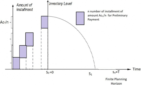
Due to no shortage, before the previous inventory level reaches zero, the retailer orders their products from the supplier. The supplier will then immediately replenish his order, with the same quantity as products ordered. Length of the cycle (T) varies in finite planning horizon. The amount of quantity (Ri+1) ordered is also not constant. The differential equation that represents the changes in inventory level is represented by the figure of inventory level (Figure 1).
Figure 1. Preliminary payment by Wu and Zhao [29]
$\frac{\left(I L_{i+1}(t)\right)}{d t}=-D(P, G)-\theta * I L_{i+1}(t)$ (1)
where, si≤t≤si+1.
$I L_{i+1}(t)=e^{-\theta t} \int_{t}^{s_{i+1}}(P, G) e^{\theta u} d u$ (2)
See Appendix.
where, ILi+1(si+1)=0 and ILi+1(si)=Ri+1.
$\mathrm{IL}_{\mathrm{i}+1}(\mathrm{t})=\int_{t}^{\mathrm{s}_{\mathrm{i}+1}}(\mathrm{P}, \mathrm{G}) \mathrm{e}^{\theta(\mathrm{u}-\mathrm{t})} \mathrm{du}$ (3)
$\mathrm{IL}_{\mathrm{i}+1}(\mathrm{t})=\frac{\mathrm{D}(\mathrm{P}, \mathrm{G})\left(\mathrm{e}^{\theta\left(\mathrm{s}_{\mathrm{i}+1}-\mathrm{t}\right)}-1\right)}{\theta}$ (4)
$R_{i+1}=I L_{i+1}\left(s_{i}\right)=e^{-\theta s_{i}} \int_{s_{i}}^{s_{i+1}}(P, G) e^{\theta t} d t$ (5)
$R_{i+1}=I L_{i+1}\left(s_{i}\right)=(P, G)\left. e^{\theta\left(s_{i+1}-s_{i}\right)}-1\right.$ (6)
Ordering cost
$O_{c}=\mathrm{m} 1 * O_{x}$ (7)
Holding cost
$H_{c}=\sum_{i=0}^{m_{1}-1} h_{c} \int_{s_{i}}^{s_{i+1}} \int_{t}^{s_{i+1}}(P, G) e^{\theta(u-t)} d u d t$ (8)
Deterioration cost
$\mathrm{Dc}=\sum_{i=0}^{m_{1}-1} \theta d_{c} \int_{s_{i}}^{s_{i+1}} \int_{t}^{s_{i+1}}(P, G) e^{\theta(u-t)} d u d t$ (9)
Carbon emission cost
$C e=\sum_{i=0}^{m_{1}-1} \mathrm{c}^{\hat{r}}+\hat{P}_{r} * R_{i+1}+\widehat{h_{c}} \int_{s_{i}}^{s_{i+1}} \int_{t}^{s_{i+1}}(P, G) e^{\theta(u-t)} d u d t$ (10)
4.1 Model for Preliminary payment under finite planning horizon
As demonstrated in Figure 2, retailer prepays the acquisition cost in n equal installments. Figure 2 displays one cycle out of several cycles in a finite planning horizon.
Figure 2. Preliminary payment by Shi et al. [9]
Acquisition cost
$\sum_{i=0}^{m_{1}-1}(1-\mathrm{r}) * P_{r} \int_{s_{i}}^{s_{i+1}}(P, G) e^{\theta\left(t-s_{i}\right)} d t$ (11)
Capital cost
$C c_{1}=\sum_{i=0}^{m_{1}-1} \frac{\mathrm{I} * \mathrm{~N}(\mathrm{n}+1)(1-\mathrm{r}) * P_{r}}{2 n} \int_{s_{i}}^{s_{i+1}}(P, G) e^{\theta\left(t-s_{i}\right)} d t$ (12)
Interest charges
$I c_{1}=\sum_{i=0}^{m_{1}^{-1}} I(1-r) P_{r} \int_{s_{i}}^{s_{i+1}} \int_{t}^{s_{i+1}}(P, G) e^{\theta(u-t)} d u$ (13)
Retailers overall cost
Total costTCR1=Ordering cost+ holding Cost + deterioration cost + Aquation cost + capital cost+ charges intrest + carbon cost.
$T C R_{1}=m_{1} * O_{c}+(1-r) * P_{r} \sum_{i=0}^{m_{1}-1} \int_{s_{i}}^{s_{i+1}}(P, G) e^{\theta\left(t-s_{i}\right)} d t$
$+\sum_{i=0}^{m_{1}-1} \frac{\mathrm{I} * \mathrm{~N}(\mathrm{n}+1)(1-\mathrm{r}) * P_{r}}{2 n} \sum_{i=0}^{m_{1}-1} \int_{s_{i}}^{s_{i+1}}(P, G) e^{\theta\left(t-s_{i}\right)} d t$
$+\sum_{i=0}^{m_{1}-1} I(i-r) P_{r} * \int_{s_{i}}^{s_{i+1}} \int_{t}^{s_{i+1}}(P, G) e^{\theta(u-t)} d u d t$
$+\sum_{i=0}^{m_{1}-1} h_{c} \int_{s_{i}}^{s_{i+1}} \int_{t}^{s_{i+1}}(P, G) e^{\theta(u-t)} d u d t$
$+\sum_{i=0}^{m_{1}-1} \theta d_{c} \int_{s_{i}}^{s_{i+1}} \int_{t}^{s_{i+1}}(P, G) e^{\theta(u-t)} d u d t+\sum_{i=0}^{m_{1}-1} \tau\left(Z-\left(\mathrm{c}^{\wedge}+\hat{P}_{r}\right.\right.$
$\left.\left.* R_{i+1}+\widehat{h_{c}} \int_{s_{i+1}}^{s_{i}} \int_{t}^{s_{i+1}}(P, G) e^{\theta(u-t)} d u d t\right)\right)$ (14)
$\frac{\partial T C R_{1}}{\partial s_{i}}=\left\{\left\{(1-r) * P_{r}+\frac{\mathrm{I} * \mathrm{~N}(\mathrm{n}+1)(1-\mathrm{r}) * P_{r}}{2 n}-\tau \hat{P}_{r}\right\}\right.$
$\left.+\frac{\left\{I(1-r) P_{r}-\widehat{h_{c}} \mathrm{\tau}+h_{c}+\theta d_{c}\right\}}{\theta}\right\} D(P, G) \sum_{i=0}^{m_{1}-1}\left\{e^{\theta\left(s_{i}-s_{i-1}\right)}\right.\left.-e^{\theta\left(s_{i+1}-s_{i}\right)}\right\}$ (15)
$\frac{\partial^{2} T C R_{1}}{\partial s_{i}{ }^{2}}=\left\{\left\{(1-r) * P_{r}+\frac{\mathrm{I} * \mathrm{~N}(\mathrm{n}+1)(1-\mathrm{r}) * P_{r}}{2 n}-\tau \hat{P}_{r}\right\}\right.$
$\left.+\frac{\left\{I(1-r) P_{r}-\widehat{h}_{c} \tau+h_{c}+\theta d_{c}\right\}}{\theta}\right\} D(P, G) \theta \sum_{i=0}^{m_{1}-1}\left\{e^{\theta\left(s_{i}-s_{i-1}\right)}\right.\left.+e^{\theta\left(s_{i+1}-s_{i}\right)}\right\}$ (16)
$\frac{\partial^{2} T C R_{1}}{\partial\left(s_{i}\right)\left(s_{i-1}\right)}=\left\{\left\{(1-r) * P_{r}+\frac{\mathrm{I} * \mathrm{~N}(\mathrm{n}+1)(1-\mathrm{r}) * P_{r}}{2 n}-\tau \hat{P}_{r}\right\}\right.$
$\left.+\frac{\left\{I(1-r) P_{r}-\widehat{h_{c}} \mathrm{\tau}+h_{c}+\theta d_{c}\right\}}{\theta}\right\} D(P, G) \sum_{i=0}^{m_{1}-1}-\theta\left\{e^{\theta\left(s_{i}-s_{i-1}\right)}\right\}$ (17)
$\frac{\partial^{2} T C R_{1}}{\partial\left(s_{i}\right)\left(s_{i+1}\right)}=\left\{\left\{(1-r) * P_{r}+\frac{\mathrm{I} * \mathrm{~N}(\mathrm{n}+1)(1-\mathrm{r}) * P_{r}}{2 n}-\tau \hat{P}_{r}\right\}\right.$
$\left.+\frac{\left\{I(1-r) P_{r}-\widehat{h_{c}} \mathrm{\tau}+h_{c}+\theta d_{c}\right\}}{\theta}\right\} D(P, G) \sum_{i=0}^{m_{1}-1} \theta\left\{e^{\theta\left(s_{i+1}-s_{i}\right)}\right\}$ (18)
$\frac{\partial^{2} T C R_{1}}{\partial\left(s_{i}\right)\left(s_{n}\right)}=0$ f or all $\mathrm{n}$ is $\mathrm{i}-1, \mathrm{i}+1, \quad$ and $\mathrm{I}$ (19)
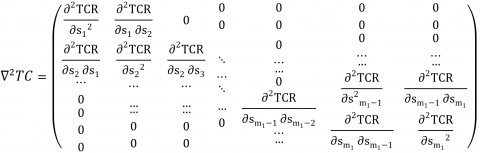
By Singh et al. [13, 15] and Sarkar et al. [31] the fact that the Hessian matrix of TCR is positive definite is sufficient for a total cost to be min as given in Figure 3.
Figure 3. Hesian matrix Sarkar et al. [31]
Condition to check positive definite:
$\begin{aligned} &\left|\frac{\partial^{2} T C R_{1}\left(m_{1}, s_{0}, s_{1} \ldots \ldots \ldots \ldots \ldots s_{m}\right)}{\partial s_{i}^{2}}\right| \\ &\geq\left|\frac{\partial^{2} T C R_{1}\left(m_{1}, s_{0}, s_{1} \ldots \ldots \ldots \ldots \ldots s_{m}\right)}{\partial\left(s_{i}\right)\left(s_{i-1}\right)}\right| \\ &+\left|\frac{\partial^{2} T C R_{1}\left(m_{1}, s_{0}, s_{1} \ldots \ldots \ldots \ldots \ldots s_{m}\right)}{\partial\left(s_{i}\right)\left(s_{i+1}\right)}\right| \end{aligned}$
$\left|\frac{\partial^{2} T C R_{1}\left(m_{1}, s_{0}, s_{1} \ldots \ldots \ldots \ldots \ldots s_{m}\right)}{\partial s_{i}^{2}}\right|-$
$\left|\frac{\partial^{2} T C R_{1}\left(m_{1}, s_{0}, s_{1} \ldots \ldots \ldots \ldots \ldots . \ldots s_{m}\right)}{\partial\left(s_{i}\right)\left(s_{i-1}\right)}\right|-$
$\left|\frac{\partial^{2} T C R_{1}\left(m_{1}, s_{0}, s_{1} \ldots \ldots \ldots \ldots \ldots s_{m}\right)}{\partial\left(s_{i}\right)\left(s_{i+1}\right)}\right| \geq 0$ (20)
Model for cash payment under finite planning horizon.
Acquisition cost
$A c_{2}=\sum_{i=0}^{m_{1}-1} P_{r} \int_{s_{i}}^{s_{i+1}}(P, G) e^{\theta\left(t-s_{i}\right)} d t$ (21)
Interest charges
$I c_{2}=\sum_{i=0}^{m_{1}-1} I * P_{r} \int_{s_{i}}^{s_{i+1}} \int_{t}^{s_{i+1}} D(P, G) e^{\theta(u-t)} d u d t$ (22)
Retailer’s overall cost
Total cost TCR2=Ordering cost + holding Cost + deterioration cost + Aquation cost + charges interest + carbon cost
$T C R_{2}=m_{1} * O_{c}+P_{r} \sum_{i=0}^{m_{1}-1} \int_{s_{i}}^{s_{i+1}} D(P, G) e^{\theta\left(t-s_{i}\right)} d t+I$
$* P_{r} \sum_{i=0}^{m_{1}-1} \int_{s_{i}}^{s_{i+1}} I L_{i+1} d t$
$+h_{c} \sum_{i=0}^{m_{1}-1} \int_{s_{i}}^{s_{i+1}} I L_{i+1} d t \theta d_{c} \sum_{i=0}^{m_{1}-1{ }_{s_{i+1}}^{s_{i}}} I L_{i+1} d t \sum_{i=0}^{m_{1}-1} \tau(Z \left.-\left(\mathrm{c}^{\hat{n}}+\hat{P}_{r} * R_{i+1}+\widehat{h_{c}} \int_{s_{i}} I L_{i+1}(t) d t\right)\right)$ (23)
$T C R_{2}=m_{1} * O_{c}+\left(P_{r}-P_{r} \tau\right) \sum_{i=0}^{m_{1}-1} \int_{s_{i}}^{s_{i+1}} D(P, G) e^{\theta\left(t-s_{i}\right)} d t$
$+\left\{I * P_{r}+h_{c}+\theta d_{c}\right.$
$\left.+\widehat{h_{c}} \tau\right\} \sum_{i=0}^{m_{1}-1} \int_{s_{i}}^{s_{i+1} s_{i+1}} \int_{t} D(P, G) e^{\theta(u-t)} d u d t+Z * \tau-\hat{c} \tau$ (24)
$\begin{aligned} \frac{\partial T C R_{2}}{\partial s_{i}}=\left\{P_{r}+\right.& \frac{\mathrm{I} * P_{r}-\widehat{h_{c}} \tau+h_{c}+\theta d_{c}}{\theta}\left.-\tau \widehat{P}_{r}\right\} D(P, G) \sum_{i=0}^{m_{1}-1}\left\{e^{\theta\left(s_{i}-s_{i-1}\right)}\right.\left.-e^{\theta\left(s_{i+1}-s_{i}\right)}\right\} \end{aligned}$ (25)
4.2 Model for post payment under finite planning horizon
In general, according to the market norm, the simplest method is to purchase a product and pay for it. Yet, Trade Credit is a practical choice for the majority of firms. In this case, the supplier gives the retailer a set amount of time to pay for the purchases. within this permissible limit, there are no losses for the supplier. Sometimes, to reduce the risk of default, the supplier usually offers a discount to promote early payment. Therefore, the retailer is given a specified credit period Mrby the supplier to the retailer in this situation.
The realtor’s acquisition cost per replenishment cycle time Ti+1 shown clearly by:
Acquisition cost
$A c_{3}=\sum_{i=0}^{m_{1}-1} P_{r} \int_{s_{i}}^{s_{i+1}}(P, G) e^{\theta\left(t-s_{i}\right)} d t$ (26)
Interest charges
$I c_{3}=\sum_{i=0}^{m_{1}-1} I * P_{r} \int_{M}^{s_{i+1}} \int_{t}^{s_{i+1}} D(P, G) e^{\theta(u-t)} d u d t$ (27)
Sub-case 1 of Mc ≤ T s
Since Mc≤T, the retailer in this sub-case must pay interest on the products in stock after time Mc
The interest charged per cycles:
$\mathrm{TCR}_{3} I E_{31}=I * I_{e} * S * D(P, G) M_{C}^{2}$ (28)
$T C R_{3}=m_{1} * O_{c}+\left(P_{r}-P_{r} \tau\right) \sum_{i=0}^{m_{1}-1} \int_{s_{i}}^{i+1} D(P, G) e^{\theta\left(t-s_{i}\right)} d t$
$+\left\{I * P_{r}+h_{c}+\theta d_{c}\right.$
$\left.-\widehat{h_{c}} \tau\right\} \sum_{i=0}^{m_{1}-1} \int_{s_{i}}^{s_{i+1}} \int_{t}^{s_{i+1}} D(P, G) e^{\theta(u-t)} d u d t+Z * \tau -\mathrm{c}^{\wedge} \tau-\left\{\mathrm{I} * I_{e} * \mathrm{~s} * \mathrm{D}(\mathrm{P}, \mathrm{G}) * M^{2}\right\}$ (29)
4.2.1 Model for Preliminary payment under finite planning horizon
The interest charged per cycles:
$I E_{32}=\sum_{i=0}^{m_{1}-1} I_{e} * S * D(P, G) T_{i+1}\left\{M_{c}-\frac{1}{2} T_{i+1}\right\}$ (30)
Interest charges $\left(I C_{32}\right)=0$ (31)
Retailers overall cost
Total cost (TCR32) =Ordering Cost+ Holding Cost + Deterioration Cost + Aquation cost+ Charges Interest- Interest Earn+ Carbon Cost
$T C R_{32}=m_{1} * O_{c}+P_{r} \sum_{i=0}^{m_{1}-1} \int_{s_{i}}^{s_{i+1}} D(P, G) e^{\theta\left(t-s_{i}\right)} d t+I *$
$P_{r} \sum_{i=0}^{m_{1}-1} \int_{M_{c}}^{s_{i+1}} I L_{i+1} d t+$
$h_{c} \sum_{i=0}^{m_{1}-1} \int_{s_{i}}^{s_{i+1}} I L_{i+1} d t+\theta d_{c} \sum_{i=0}^{m_{1}-1} \int_{s_{i}}^{s_{i+1}} I L_{i+1} d t+\sum_{i=0}^{m_{1}-1} \tau(Z-$
$\left.\left(c^{\wedge}+\hat{P}_{r} * R_{i+1}+\widehat{h_{c}} \int_{s_{i}}^{s_{i+1}} I L_{i+1}(t) d t\right)\right)-\sum_{i=0}^{m_{1}-1} I_{e} * s *$
$D(P, G) T_{i+1}\left\{M_{c}-\frac{1}{2} T_{i+1}\right\}$ (32)
$\begin{aligned} T C R_{32}=m_{1} * O_{c}+\left(P_{r}\right.&\left.-P_{r} \tau\right) \sum_{i=0}^{m_{1}-1} \int_{s_{i}}^{s_{i+1}} D(P, G) e^{\theta\left(t-s_{i}\right)} d t \\ &+\left\{h_{c}+\theta d_{c}-\widehat{h_{c}} \tau\right\} \\ &+\sum_{i=0}^{m_{1}-1} \int_{s_{i} s_{i+1} s_{i+1}} \int_{t} D(P, G) e^{\theta(u-t)} d u d t \\ &+Z * \tau-c^{n} \tau \\ &-\sum_{i=0}^{m_{1}-1} I_{e} * s \\ & * D(P, G)\left\{s_{i+1}-s_{i}\right\}\left\{M_{c}\right. \left.-\frac{1}{2}\left\{s_{i+1}-s_{i}\right\}\right\} \end{aligned}$ (33)
$R_{(i+1)}=\sum_{i=0}^{m_{1}^{*}-1} R_{i+1}^{*}$ (34)
Supplier total cost is given by the following equation.
$T C S=m_{1}^{*} S_{c}+\sum_{i=0}^{m_{1}^{*}-1} P_{r} * R_{i+1}^{*}$ (35)
Step 1: Create a new set of inputs: Oc, Dt, Hc, Ss, Ac, Cc, Ic, Ie, Pr, cˆ, Pˆr, hˆc, N, r, n, Mc, θ, … …. …. …τ, Ce, Ti+1, T etc.
Step 2: The forecasted total cost TCR (cost of retailer) and TCS (total cost of supplier) is a function of si, which may be calculated numerically.
Now, using the given input values in step 1, compute the values of si from the preceding equations $\frac{\partial \mathrm{TCR}}{\partial \mathrm{s}_{\mathrm{i}}}$=0 using the given input values in step 1.
Step 3: After calculating the si values in step 2, verify the condition: $\left|\frac{\partial^{2} \mathrm{TCR}}{\partial \mathrm{s}_{\mathrm{i}}^{2}}\right| \geq\left|\frac{\partial^{2} \mathrm{TCR}}{\partial\left(\mathrm{s}_{\mathrm{i}}\right)\left(\mathrm{s}_{\mathrm{i}-1}\right)}\right|+\left|\frac{\partial^{2} \mathrm{TCR}}{\partial\left(\mathrm{s}_{\mathrm{i}}\right)\left(\mathrm{s}_{\mathrm{i}+1}\right)}\right|$.
Step 4: Determine the most appropriate TCR values which will be the optimal expected average cost by Using the values of si obtained in step 3.
Step 5: Using the values of si obtained in step 2 and the equation given below, by which we will determine optimal order quantity. $R_{(i+1)}=\sum_{i=0}^{m_{1}^{*}-1} R_{i+1}^{*}$.
Step 6: After 5th step we can find TCS (Supplier total cost) which depend upon retailer replenish- ment policy.
Numerical data: This section give an information about numerical data; we’ll look at a numerical data to illustrate how various factors affect the overall cost of retailer’s and suppliers. Let a=0.15, n=10, r=0.5, hd=10, b=0.000001, c=0.0001, W=4, I=0.1, Sr=350, Ss=400, θ=2, cˆ=1, hc=2, hˆc =0.2, Cc=5, P=1, G=1, N=0.17, Mr=0.17, Ie=0.08, s=50, τ= 0.5, g= 0.00001, dc=1, Z = 0.002, Pr= 0.02, Pˆr=10 with the appropriate units. We will use Mathematica software(version-12) to solve Non-linear Eqns. (20) and (24). we can see tabulation and graphically presentation of the overall cost of suppliers and retailers and optimal quantity all of the different parameters and replacement cycles, i.e. for m1−1=1, 2, 3, and so on.
As according to Table 2 and Figure 4, if the value of r (the discount rate for preliminary payment) rises, the retailer’s and supplier’s overall cost remain constant. This result implies that with the increasing discount rate in the case of advance payment, no of ordering quantity decrease. As a result, has no relationship with overall retailer’s and supplier’s cost and a direct relationship with the number of replenishment cycles.
Table 2. Table for changes in r(discount rate)for Pre- liminary Payment under finite planning horizon
|
r |
Ri+1 |
TCR1 |
TCS1 |
|
0.240 |
3170.76 |
3.6054 ∗ 107 |
751125.74 |
|
0.245 |
3170.10 |
3.6054 ∗ 107 |
751125.74 |
|
0.250 |
3169.43 |
3.6054 ∗ 107 |
751125.74 |
|
0.255 |
3168.77 |
3.6054 ∗ 107 |
751125.74 |
|
0.260 |
3168.11 |
3.6054 ∗ 107 |
751125.74 |
In Table 3, Table 4 and their graphically presentation by Figure 5, Figure 6, Figure 7 and Figure 8 an increase in an (initial demand) increases the retailer, supplier, and order quantity as well. It is obvious the higher the initial demand the higher the order as well as TCR and TCS for all types of payment.
As per Table 3, Table 4, Figure 5, Figure 6, Figure 7 and Figure 8, if there is an increase in the value of θ (deterioration rate of the inventory) for the case of advance payment, the total cost of the retailer starts decreasing and total cost of retailer start increase. But, with the increase in the value of θ and the replenishment quantity, the total cost decreases which implies that if the inventory is replenished more frequently, the deterioration rate is less and so is the total cost. Thus, θ is directly related to total supplier cost and order quantity and indirectly with the total retailer cost. Similarly for credit payment in the case of Mc ≥ Ti ′s But, in cash payment and for the case Mc ≤ Ti ′s, θ is directly related to the total retailer, supplier cost, and order quantity.
Table 4 and Figure 8 explains the link between Mc(trade credit period) and finite planning horizon (T). Because the credit duration is longer than Ti, the retailer will have the more time to settle the entire payment, will extend the interest earned period.
As a result, the retailer’s earnings will rise, resulting in a reduction in total cost. and vice versa in case for Mc≤Ti′. Table 4 shows the sensitivity analysis for different parameters.
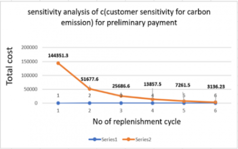
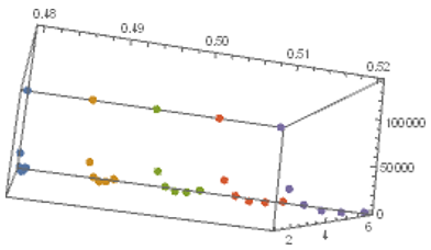
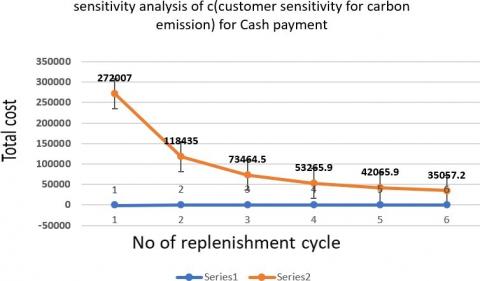
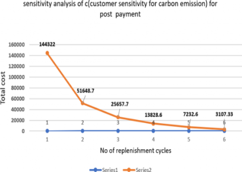
As c is the consumer’s sensitivity to carbon emissions per unit and when carbon emissions per unit product rise by one unit demand falls by c. as an increase in value of c in Table 4; Table 3 then there are no changes in Ri+1, TCR and TCS. But their graphical presentation in Figure 5, Figure 6, Figure 7 and Figure 8 analysis a decrease in carbon emission to its original value, and as a result total cost also decreases for a different payment scheme.
Table 3. Table for preliminary and cash payment under finite planning horizon
|
|
Preliminary payment |
Cash payment |
||||
|
Ri+1 |
TCR |
TCS |
Ri+1 |
TCR |
TCS |
|
|
a=240 |
360546.74 |
2799.04 |
9610.93 |
360533.82 |
18095.7 |
9610.68 |
|
a=245 |
368057.87 |
2805.52 |
9761.16 |
368044.94 |
18421.9 |
9760.90 |
|
a=250 |
375569.01 |
2812.00 |
9911.38 |
375556.07 |
18748.0 |
9911.12 |
|
a=255 |
383081.49 |
2822.67 |
10061.60 |
383067.19 |
19074.2 |
10061.30 |
|
a=260 |
390592.60 |
2829.06 |
10211.90 |
390578.32 |
19400.4 |
10211.60 |
|
c=0.48 |
3136.23 |
3.6054*107 |
751125.81 |
751112.36 |
35057.21 |
3.60534 ∗ 107 |
|
c=0.49 |
3136.23 |
3.6054*107 |
751125.81 |
751112.36 |
35057.21 |
3.60534 ∗ 107 |
|
c=0.50 |
3136.23 |
3.6054*107 |
751125.81 |
751112.36 |
35057.21 |
3.60534 ∗ 107 |
|
c=0.51 |
3136.23 |
3.6054*107 |
751125.81 |
751112.36 |
35057.21 |
3.60534 ∗ 107 |
|
c-0.52 |
3136.23 |
3.6054*107 |
751125.81 |
751112.36 |
35057.21 |
3.60534 ∗ 107 |
|
θ =0.96 |
28455.16 |
4672.37 |
1.36585 ∗ 106 |
28399.4 |
27189.4 |
1.36317 ∗ 106 |
|
θ =0.98 |
29963.13 |
4644.08 |
1.43823 ∗ 106 |
29909.7 |
27316.6 |
1.43567 ∗ 106 |
|
θ =1.00 |
31573.39 |
4616.31 |
1.51552 ∗ 106 |
31522.2 |
27444.8 |
1.51307 ∗ 106 |
|
θ =1.02 |
33307.18 |
4657.70 |
1.59875 ∗ 106 |
33244.0 |
27573.7 |
1.59571 ∗ 106 |
|
θ =1.04 |
35143.25 |
4626.32 |
1.68688 ∗ 106 |
35082.9 |
27703.5 |
1.68398 ∗ 106 |
|
τ = 0.240 |
751139.32 |
20001.30 |
3.60547*107 |
751112.29 |
35140.5 |
3.60547 ∗ 107 |
|
τ =0.245 |
751138.79 |
19674.40 |
3.60547 ∗ 107 |
751112.29 |
35138.90 |
3.60547 ∗ 107 |
|
τ =0.250 |
751138.27 |
19347.70 |
3.60547 ∗ 107 |
751112.29 |
35137.30 |
3.60547 ∗ 107 |
|
τ =0.255 |
751140.46 |
19037.70 |
3.60547 ∗ 107 |
751112.29 |
35135.70 |
3.60547 ∗ 107 |
|
τ =0.260 |
751139.88 |
18710.60 |
3.60547 ∗ 107 |
751112.29 |
35134.10 |
3.60547 ∗ 107 |
|
pˆr =4.8 |
751139.26 |
19922.60 |
3.60547 ∗ 107 |
751112.29 |
35062.80 |
3.60534 ∗ 107 |
|
pˆr =4.9 |
751138.73 |
19597.30 |
3.60547 ∗ 107 |
751112.29 |
35062.70 |
3.60534 ∗ 107 |
|
pˆr =5.0 |
751138.22 |
19272.10 |
3.60547 ∗ 107 |
751112.29 |
35062.50 |
3.60534 ∗ 107 |
|
pˆr =5.1 |
751140.39 |
18963.50 |
3.60547 ∗ 107 |
751112.29 |
35062.40 |
3.60534 ∗ 107 |
|
pˆr =5.2 |
751139.81 |
18637.90 |
3.60547 ∗ 107 |
751112.29 |
35062.30 |
3.60534 ∗ 107 |
|
hˆc = 20 |
751125.76 |
3214.06 |
17422.51 |
751112.29 |
35134.70 |
17422.20 |
|
hˆc = 20 |
751125.76 |
3212.56 |
17422.51 |
751112.29 |
35133.20 |
17422.20 |
|
hˆc = 20 |
751125.76 |
3211.06 |
17422.51 |
751112.29 |
35131.70 |
17422.20 |
|
hˆc = 20 |
751125.76 |
3209.58 |
17422.51 |
751112.29 |
35130.20 |
17422.20 |
|
hˆc = 20 |
751125.76 |
3208.08 |
17422.51 |
751112.29 |
35128.70 |
17422.20 |
|
S r =20 |
751125.73 |
1862.23 |
17422.51 |
751112.29 |
33783.20 |
17422.24 |
|
S r =20 |
751125.73 |
1886.73 |
17422.51 |
751112.29 |
33807.70 |
17422.24 |
|
S r =20 |
751125.73 |
1911.23 |
17422.51 |
751112.29 |
33832.20 |
17422.24 |
|
S r =20 |
751125.73 |
1935.73 |
17422.51 |
751112.29 |
33856.70 |
17422.24 |
|
S r =20 |
751125.73 |
1960.23 |
17422.51 |
751112.29 |
33881.20 |
17422.24 |
|
S s =20 |
751125.73 |
3136.23 |
16174.50 |
751112.29 |
35057.20 |
16174.24 |
|
S s =20 |
751125.73 |
3136.23 |
16198.50 |
751112.29 |
35057.20 |
16198.24 |
|
S s =20 |
751125.73 |
3136.23 |
16222.50 |
751112.29 |
35057.20 |
16222.24 |
|
S s =20 |
751125.73 |
3136.23 |
16246.50 |
751112.29 |
35057.20 |
16246.24 |
|
S s =20 |
751125.73 |
3136.23 |
16270.50 |
751112.29 |
35057.20 |
16270.24 |
|
pr =0.0096 |
751125.71 |
3101.69 |
9610.81 |
751112.29 |
35055.63 |
9610.68 |
|
pr = 0.0098 |
751125.71 |
3102.36 |
9761.03 |
751112.29 |
35055.66 |
9760.90 |
|
pr =0.0100 |
751125.71 |
3103.02 |
9911.26 |
751112.29 |
35055.69 |
9911.12 |
|
pr =0.0102 |
751125.71 |
3103.68 |
10061.50 |
751112.29 |
35055.72 |
10061.30 |
|
pr =0.0104 |
751125.71 |
3104.34 |
10211.70 |
751112.29 |
35055.75 |
10211.60 |
|
b=4.8*10−7 |
3136.23 |
3.6054*107 |
751125.73 |
35057.20 |
3.60534*107 |
751112.29 |
|
b=4.9*10−7 |
3136.23 |
3.6054*107 |
751125.73 |
35057.20 |
3.60534*107 |
751112.29 |
|
b=5.0*10−7 |
3136.23 |
3.6054*107 |
751125.73 |
35057.20 |
3.60534*107 |
751112.29 |
|
b=5.1*10−7 |
3136.23 |
3.6054*107 |
751125.73 |
35057.20 |
3.60534*107 |
751112.29 |
|
b=5.2*10−7 |
3136.23 |
3.6054*107 |
751125.73 |
35057.20 |
3.60534*107 |
751112.29 |
Table 4. Table for post payment under finite planning horizon
|
Parameters Post payment for Mc≤Ti′ s |
Post payment for Mc ≥T |
|||||
|
|
Ri+1 |
TCR |
TCS |
Ri+1 |
TCR |
TCS |
|
a=240 |
360533.82 |
18081.80 |
9610.68 |
1.30478 ∗ 107 |
49355.27 |
263356.50 |
|
a=245 |
368044.94 |
18407.70 |
9760.90 |
1.33197 ∗ 107 |
50335.45 |
268793.10 |
|
a=250 |
375556.07 |
18733.60 |
9911.12 |
1.35915 ∗ 107 |
51315.63 |
274229.70 |
|
a=255 |
383067.19 |
19059.50 |
10061.30 |
1.38633 ∗ 107 |
52295.80 |
279666.29 |
|
a=260 |
390578.32 |
19385.40 |
10211.60 |
1.41351 ∗ 107 |
53275.98 |
285102.89 |
|
c=0.48 |
751125.81 |
3107.33 |
3.6054 ∗ 107 |
2.7183 ∗ 107 |
100324.45 |
1.30478 ∗ 109 |
|
c=0.49 |
751125.81 |
3107.33 |
3.6054 ∗ 107 |
2.7183 ∗ 107 |
100324.45 |
1.30478 ∗ 109 |
|
c=0.50 |
751125.81 |
3107.33 |
3.6054 ∗ 107 |
2.7183 ∗ 107 |
100324.45 |
1.30478 ∗ 109 |
|
c= 0.51 |
751125.81 |
3107.33 |
3.6054 ∗ 107 |
2.7183 ∗ 107 |
100324.45 |
1.30478 ∗ 109 |
|
c=0.52 |
751125.81 |
3107.33 |
3.6054 ∗ 107 |
2.7183 ∗ 107 |
100324.45 |
1.30478 ∗ 109 |
|
θ =0.96 |
28399.40 |
27160.50 |
1.36317 ∗ 106 |
56941.20 |
48815.80 |
2.73318 ∗ 106 |
|
θ =0.98 |
29909.70 |
27287.70 |
1.36317 ∗ 106 |
61934.60 |
49388.30 |
2.97286 ∗ 106 |
|
θ =1.00 |
31522.20 |
27415.90 |
1.36317 ∗ 106 |
67479.40 |
49971.40 |
3.23901 ∗ 106 |
|
θ =1.02 |
33244.00 |
27544.80 |
1.36317 ∗ 106 |
67718.50 |
49244.1 |
3.25049 ∗ 106 |
|
θ =1.04 |
35082.90 |
27674.6 |
1.36317 ∗ 106 |
73836.00 |
49821.6 |
3.54413 ∗ 106 |
|
Pˆr =4.8 |
751112.29 |
35033.86 |
3.60534 ∗ 107 |
8.49346 ∗ 106 |
74212.8 |
4.07686 ∗ 108 |
|
Pˆr =4.9 |
751112.29 |
35033.75 |
3.60534 ∗ 107 |
8.62455 ∗ 106 |
74519.80 |
4.13978 ∗ 108 |
|
Pˆr =5.0 |
751112.29 |
35033.64 |
3.60534 ∗ 107 |
8.75935 ∗ 106 |
74831.60 |
4.20449 ∗ 108 |
|
Pˆr =5.1 |
751112.29 |
35033.54 |
3.60534 ∗ 107 |
8.89799 ∗ 106 |
75148.30 |
4.27103 ∗ 108 |
|
Pˆr =5.2 |
751112.29 |
35033.43 |
3.60534 ∗ 107 |
9.04062 ∗ 106 |
75469.90 |
4.3395 ∗ 108 |
|
τ = 0.240 |
751112.29 |
35111.56 |
3.60534 ∗ 107 |
8.69148 ∗ 106 |
74841.00 |
4.17191 ∗ 108 |
|
τ =0.245 |
751112.29 |
35109.96 |
3.60534 ∗ 107 |
8.82956 ∗ 106 |
75155.90 |
4.23819 ∗ 108 |
|
τ =0.250 |
751112.29 |
35108.36 |
3.60534 ∗ 107 |
8.97165 ∗ 106 |
75475.70 |
4.30639 ∗ 108 |
|
τ =0.255 |
751112.29 |
35106.76 |
3.60534 ∗ 107 |
8.4267 ∗ 106 |
74204.00 |
4.04482 ∗ 108 |
|
τ =0.260 |
751112.29 |
35105.16 |
3.60534 ∗ 107 |
8.55724*106 |
74509.10 |
4.10747 ∗ 108 |
|
S r = 168.0 |
751112.29 |
33754.30 |
3.60534 ∗ 107 |
2.7183 ∗ 107 |
99050.40 |
1.30478 ∗ 109 |
|
S r =171.5 |
751112.29 |
33778.80 |
3.60534 ∗ 107 |
2.7183 ∗ 107 |
99074.90 |
1.30478 ∗ 109 |
|
S r =175.0 |
751112.29 |
33803.30 |
3.60534 ∗ 107 |
2.7183 ∗ 107 |
99099.40 |
1.30478 ∗ 109 |
|
S r =178.5 |
751112.29 |
33827.80 |
3.60534 ∗ 107 |
2.7183 ∗ 107 |
99123.90 |
1.30478 ∗ 109 |
|
S r = 182.0 |
751112.29 |
33852.30 |
3.60534 ∗ 107 |
2.7183 ∗ 107 |
99148.40 |
1.30478 ∗ 109 |
|
S s =192 |
751112.29 |
35028.30 |
16174.2 |
2.7183 ∗ 107 |
100324.44 |
544812.51 |
|
S s =196 |
751112.29 |
35028.30 |
16198.2 |
2.7183 ∗ 107 |
100324.44 |
544836.51 |
|
S s =200 |
751112.29 |
35028.30 |
16222.2 |
2.7183 ∗ 107 |
100324.44 |
544860.51 |
|
S s =204 |
751112.29 |
35028.30 |
16246.2 |
2.7183 ∗ 107 |
100324.44 |
544884.51 |
|
S s = 208 |
751112.29 |
35028.30 |
16270.2 |
2.7183 ∗ 107 |
100324.44 |
544908.51 |
|
pr =0.0096 |
751112.29 |
35026.73 |
9610.67 |
25.8932 |
346.288 |
400.518 |
|
pr =0.0098 |
751112.29 |
35026.76 |
9760.90 |
26.4383 |
346.437 |
400.529 |
|
pr =0.0100 |
751112.29 |
35026.79 |
9911.12 |
26.9835 |
346.586 |
400.540 |
|
pr =0.0102 |
751112.29 |
35026.82 |
10061.34 |
27.5287 |
346.735 |
400.551 |
|
pr =0.0104 |
751112.29 |
35026.85 |
10211.56 |
28.0739 |
346.884 |
400.561 |
|
b= 4.8 ∗10−7 |
751112.29 |
35028.31 |
3.60534 ∗ 107 |
2.7183 ∗ 107 |
100324.44 |
1.30478 ∗ 109 |
|
b= 4.9 ∗ 10−7 |
751112.29 |
35028.31 |
3.60534 ∗ 107 |
2.7183 ∗ 107 |
100324.44 |
1.30478 ∗ 109 |
|
b=5.0 ∗ 10−7 |
751112.29 |
35028.31 |
3.60534 ∗ 107 |
2.7183 ∗ 107 |
100324.44 |
1.30478 ∗ 109 |
|
b= 5.1 ∗ 10−7 |
751112.29 |
35028.31 |
3.60534 ∗ 107 |
2.7183 ∗ 107 |
100324.44 |
1.30478 ∗ 109 |
|
b= 5.2 ∗ 10−7 |
751112.29 |
35028.31 |
3.60534 ∗ 107 |
2.7183 ∗ 107 |
100324.44 |
1.30478 ∗ 109 |
An increase in Sr(ordering cost) No changes in order cost as well supplier cost. But we can see a little change in retailer cost with the help of Table 4 and Table 3. Retailer total cost will be increased.
Table 3 and Table 4 gives the detail of the relationship between S s(supplier set up cost) and Ri+1, TCR and TCS. This case is directly opposite of S r. Here, changes occur in supplier cost only.
Table 4 and Table 3 shows that independently of the choice of parameter K; cˆh; ch;τ; Pˆr; Pr; b; for different value, the optimal solutions for Preliminary, post and payments on delivery retain the following relationship: TCR1≤TCR2≤TCR3 and Ri+1.
The demand in this study is based on carbon emissions, which is also extremely realistic in the actual world. The demand for a product may not always be constant. When demand for some items that produce a lot of carbon falls, so does the rate of emission. To achieve a high degree of carbon emission reduction in the supply chain, retailers should pay more attention to the carbon awareness of the circular economy, and suppliers and manufacturers should work harder to increase carbon emission reduction efficiency. Because some items, such as medications or other commodities, deteriorate with time, suppliers and manufacturers benefit from earlier payment for a variety of reasons. To ensure that the order can be fulfilled on time, the manufacturer provides an advance payment. The provider gives a discount, a credit, or some other type of incentive in return for the early payment. As per the proposed model, in the supply chain with advance payment and carbon dependent demand, a high degree of efficiency in the supplier and manufacturer’s carbon emission reduction, as well as an increase in buyers’ carbon awareness, can encourage the supplier or manufacturer to achieve greater carbon emission reduction. To encourage business growth and the development of the circular economy, supply chains members such as retailers, suppliers and manufacturers should understand the determinants of their judgment strategies during the supply chain process.
The government has a major role to play in encouraging the creation and management of the circular economy throughout the supply chain. The government’s actions have a significant impact on supply chain partners’ decision- making.
In our proposed model, we have focused on three different models that used carbon tax and cap regulations, which support the government in assigning carbon emission caps to industries to encourage them to reduce carbon emissions.
Our findings will help the government create carbon reduction regulations to help companies reduce carbon emissions and promote a sustainable business strategy.
Comparison study
To compare the proposed model to that of Shi et al. [9], in which the parameter values are the same as in Shi et al. [9] model (Table 5). Furthermore, the values of all of the additional parameters are introduced in Example. 1 of the current model.
In this comparison study, we can conclude that our proposed model tries to minimize retailer, supplier and carbon emission costs. This occurrence opposes Shi's observations. Therefore, the proposed model is more effective in comparison to the Shi model which is economical as well as environmentally sensitive.
Table 5. Comparison chart
|
|
|
R |
|
Ri+1 |
TCR1 |
TCS1 |
Ce |
|
Proposed model |
|
0.05 |
|
751126. |
3196. |
3.605403×10⁷ |
0.331594 |
|
ti |
0.668112 |
1.33565 |
2.0026 |
2.66898 |
3.33478 |
4. |
|
|
|
0.10 |
|
751126. |
3189.36 |
3.605403×10⁷ |
0.331595 |
|
|
|
0.20 |
|
751126. |
3176.08 |
3.605403×10⁷ |
0.331598 |
|
|
|
0.30 |
|
751126. |
3162.79 |
3.605403×10⁷ |
0.3316 |
|
|
|
0.40 |
|
751126. |
3149.51 |
3.605403×10⁷ |
0.331603 |
|
|
Shi et al. [9] model |
|
R |
T2 |
Q2 |
TC2 |
- |
Ce |
|
|
0.05 |
0.248 |
978.25 |
37300 |
- |
21875 |
|
|
|
0.10 |
0.253 |
999.14 |
35687 |
- |
21917 |
|
|
|
0.20 |
0.264 |
1045.30 |
32451 |
- |
22014 |
|
|
|
0.30 |
0.276 |
1098.80 |
29198 |
- |
22130 |
|
|
|
0.40 |
0.290 |
1161.50 |
25926 |
- |
22271 |
This research proposed a supplier retailer inventory model in which: (1) the seller provides the retailer the three-payment scheme (2) some products deteriorate at a fixed rate (3) there is a fixed carbon tax to stimulate enterprises to minimize carbon emissions and slow global climate change. Theoretical findings have then shown that for each of these parameters, there is a unique optimal solution to the issue. Numerical examples have also been conducted to show the concept under these different parameters.
Finally, sensitivity studies are used to investigate the effects of critical parameters on ordering behaviors, as well as the optimal overall retailer and supplier cost per unit time. The correlations between an important parameter and the optimal solution have also been studied. Future studies might take this study in a variety of directions. First, we may broaden the scope of the carbon-tax policy under consideration here to include a variety of additional carbon-tax rules (e.g., cap-and- trade, carbon offset, etc.) that could have a different impact on purchasers’ ordering behavior. Second, this intended study might be expanded to include fuzzy in the future. It’s also possible to include parameters such as trade credit, demand based on price, and demand based on advertising. Third, this study has only one goal: to reduce the overall store and supplier cost per unit of time. A multi-criteria decision analysis reducing both total relevant cost and carbon emissions at the same time would be an interesting and important study. The supplier-retailer coordination is only conducted to identify the trade credit period.
Solution of Eq. (2).
$\frac{\left(I L_{i+1}(t)\right)}{d t}=-D(P, G)-\theta * I L_{i+1}(t)$
where, $s_{i} \leq t \leq s_{i+1}$.
Integrating factor $=e^{\int \theta d t}=e^{\theta t}$.
Thus, solution will be given as:
$-I L_{i+1}(t) e^{\theta t}=-\int_{t}^{s_{i+1}} D(P, G) e^{\theta u} d u$
$I L_{i+1}(t)=e^{-\theta t} \int_{t}^{s_{i+1}} D(P, G) e^{\theta u} d u$
[1] Toptal, A., O¨zlu¨, H., Konur, D. (2014). Joint decisions on inventory replenishment and emission reduction investment under different emission regulations. International journal of production research, 52(1): 243-269. https://doi.org/10.1080/00207543.2013.836615
[2] Rout, C., Paul, A., Kumar, R.S., Chakraborty, D., Goswami, A. (2020). Cooperative sustainable supply chain for deteriorating item and imperfect production under different carbon emission regulations. Journal of Cleaner Production, 272: 122170. https://doi.org/10.1016/j.jclepro.2020.122170
[3] Chen, X., Benjaafar, S., Elomri, A. (2013). The carbon-constrained EOQ. Operations Research Letters, 41(2): 172-179.
[4] Mishra, U., Wu, J.Z., Sarkar, B. (2021). Optimum sustainable inventory management with backorder and deterioration under controllable carbon emissions. Journal of Cleaner Production, 279: 123699. https://doi.org/10.1016/j.jclepro.2020.123699
[5] Benjaafar, S., Li, Y.Z., Daskin, M. (2012). Carbon footprint and the management of supply chains: Insights from simple models. IEEE Transactions on Automation Science and Engineering, 10(1): 99-116. https://doi.org/10.1109/TASE.2012.2203304
[6] Qin, J.J., Ren, L.G., Xia, L.G. (2017). Carbon emission reduction and pricing strategies of supply chain under various demand forecasting scenarios. Asia-Pacific Journal of Operational Research, 34(1): 1740005. https://doi.org/10.1142/S021759591740005X
[7] Aliabadi, L., Yazdanparast, R., Nasiri, M.M. (2019). An inventory model for non-instantaneous deteriorating items with credit period and carbon emission sensitive demand: A signomial geometric programming approach. International Journal of Management Science and Engineering Management, 14(2): 124-136. https://doi.org/10.1080/17509653.2018.1504331
[8] Huang, J.X. (2016). Two-Echelon supply chain decision model with price-and-carbon-emission dependent demand. International Business and Management, 12: 71-77.
[9] Shi, Y., Zhang, Z., Chen, S.C., Ca´rdenas-Barro´n, L.E., Skouri, K. (2020). Optimal replenishment decisions for perishable products under cash, advance, and credit payments considering carbon tax regulations. International Journal of Production Economics, 223: 107514. https://doi.org/10.1016/j.ijpe.2019.09.035
[10] Ghare, P., Schrader, G. (1963). An inventory model for exponentially deteriorating items. Journal of Industrial Engineering, 14(2): 238-243.
[11] Covert, R.P., Philip, G.C. (1973). An EOQ model for items with Weibull distribution deterioration. AIIE Transactions, 5(4): 323-326. https://doi.org/10.1080/05695557308974918
[12] Dye, C.Y. (2013). The effect of preservation technology investment on a non-instantaneous deteriorating inventory model. Omega, 41(5): 872-880. https://doi.org/10.1016/j.omega.2012.11.002
[13] Singh, V., Mishra, N.K., Mishra, S., Singh, P., Saxena, S. (2019). A green supply chain model for time quadratic inventory dependent demand and partially backlogging with Weibull deterioration under the finite horizon. In AIP Conference Proceedings, 2080: 060002. https://doi.org/10.1063/1.5092937
[14] Dave, U., Patel, L. (1981). (t, s i) policy inventory model for deteriorating items with time proportional demand. Journal of the Operational Research Society, 32(2): 137-142. https://doi.org/10.1057/jors.1981.27
[15] Singh, P., Mishra, N.K., Singh, V., Saxena, S. (2017). An EOQ model of time quadratic and inventory dependent demand for deteriorated items with partially backlogged shortages under trade credit. In AIP Conference Proceedings, 1860: 020037. https://doi.org/10.1063/1.4990336
[16] Pahl, J., Voß, S. (2014). Integrating deterioration and lifetime constraints in production and supply chain planning: A survey. European Journal of Operational Research, 238(3): 654-674. https://doi.org/10.1016/j.ejor.2014.01.060
[17] Dye, C.Y., Yang, C.T. (2015). Sustainable trade credit and replenishment decisions with credit- linked demand under carbon emission constraints. 244(1): 187-200. https://doi.org/10.1016/j.ejor.2015.01.026
[18] Mishra, U., Wu, J.Z., Sarkar, B. (2020). A sustainable production-inventory model for a controllable carbon emissions rate under shortages. Journal of Cleaner Production, 256: 120268. https://doi.org/10.1016/j.jclepro.2020.120268
[19] Sepehri, A., Mishra, U., Tseng, M.L., Sarkar, B. (2021). Joint pricing and inventory model for deteriorating items with maximum lifetime and controllable carbon emissions under permissible delay in payments. Mathematics, 9(5): 470. https://doi.org/10.3390/math9050470
[20] Zhang, A.X. (1996). Optimal advance payment scheme involving fixed per-payment costs. Omega, 24(5): 577-582. https://doi.org/10.1016/0305-0483(96)00023-0
[21] Taleizadeh, A.A. (2014). An EOQ model with partial backordering and advance payments for an evaporating item. International Journal of Production Economics, 155: 185-193. https://doi.org/10.1016/j.ijpe.2014.01.023
[22] Zhang, Q., Tsao, Y.C., Chen, T.H. (2014). Economic order quantity under advance payment. Applied Mathematical Modelling, 38(24): 5910-5921. https://doi.org/10.1016/j.apm.2014.04.040
[23] Teng, J.T., Ca´rdenas-Barro´n, L.E., Chang, H.J., Wu, J., Hu, Y. (2016). Inventory lot-size policies for deteriorating items with expiration dates and advance payments. Applied Mathematical Modelling, 40(19-20): 8605-8616. https://doi.org/10.1016/j.apm.2016.05.022
[24] Wu, J., Teng, J.T., Chan, Y.L. (2018). Inventory policies for perishable products with expiration dates and advance-cash-credit payment schemes. International Journal of Systems Science: Operations & Logistics, 5(4): 310-326. https://doi.org/10.1080/23302674.2017.1308038
[25] Mashud, A.H.M., Roy, D., Daryanto, Y., Chakraborty, R. K., Tseng, M.L. (2021). A controllable carbon emission and deterioration inventory model with advance payments scheme. Journal of Cleaner Production, 296: 126608. https://doi.org/10.1016/j.jclepro.2021.126608
[26] Li, L. (2016). Coordination contracts for two-echelon supply chain with price-and-carbon-emission dependent demand. Modern Economy, 7(5): 606. https://doi.org/10.4236/me.2016.75066
[27] Pang, Q., Li, M., Yang, T., Shen, Y. (2018). Supply chain coordination with carbon trading price and consumers’ environmental awareness dependent demand. Mathematical Problems in Engineering, 2018. https://doi.org/10.1155/2018/8749251
[28] Lu, C.J., Lee, T.S., Gu, M., Yang, C.T. (2020). A multistage sustainable production–inventory model with carbon emission reduction and price-dependent demand under stackelberg game. Applied Sciences, 10(14): 4878. https://doi.org/10.3390/app10144878
[29] Wu, C., Zhao, Q. (2014). Supplier–retailer inventory coordination with credit term for inventory- dependent and linear-trend demand. International Transactions in Operational Research, 21(5): 797-818. https://doi.org/10.1111/itor.12060
[30] Xu, C., Liu, X., Wu, C., Yuan, B. (2020). Optimal inventory control strategies for deteriorating items with a general time-varying demand under carbon emission regulations. Energies, 13(4): 999. https://doi.org/10.3390/en13040999
[31] Sarkar, T., Ghosh, S.K., Chaudhuri, K. (2012). An optimal inventory replenishment policy for a deteriorating item with time-quadratic demand and time-dependent partial backlogging with shortages in all cycles. Applied Mathematics and Computation, 218(18): 9147-9155. https://doi.org/10.1016/j.amc.2012.02.072