Guillermo Federico Umbricht* | Domingo Alberto Tarzia | Diana Rubio
© 2022 IIETA. This article is published by IIETA and is licensed under the CC BY 4.0 license (http://creativecommons.org/licenses/by/4.0/).
OPEN ACCESS
In this work, a bar fully insulated on its lateral surface. composed by two different unknown materials is considered. For the analytical solution, it is assumed a perfectly assembly solid-solid interface, so no heat loss due to friction is present. This is an ideal scenario, so this loss and possible measurement errors are included by simulating noisy data for the estimation of the thermal conductivity of the unknown materials. A stationary heat transfer process along the bar is considered where a Dirichlet condition is imposed at the left that represents a source of constant temperature. At the other end of the bar, a Robin condition that models heat dissipation by convection, is assumed. The constant thermal conductivity coefficients of both solids are determined under two different situations: a) two noisy temperature measurements are available, one at the interface and the other at the right boundary; b) a temperature measurement at the interface and a heat flow measurement at the right edge of the bar are given. The bounds for the errors in the identification of the unknown coefficients are obtained based on the data measurements, the room temperature and temperature values at the boundary and interface. Numerical examples are given to illustrate the ideas used for the parameter identification and elasticity analysis is carried out to measure the dependence of the data on the estimated parameters.
elasticity analysis, heat transfer, interface problem, mathematical modeling, numerical simulation, parameter estimation
Heat transfer problems in multilayer, or solid-solid interface materials, have been extensively studied in recent years due to the multiple and different applications that have been found in science and engineering [1]. These problems have direct applications in different industries, including metallurgy [2], technology and electronics [3], automotive [4], aerospace and aviation [5].
The estimation of thermal conductivity was widely studied under various approaches. Numerical techniques for inverse problems were considered in some works, for instance in [6-10]. Specifically, some authors simultaneously estimate spatially varying thermal conductivity and heat capacity, see [6]. In Ref. [7], a finite differences scheme is used while in [8] the estimation was carried out under particular conditions, using the conjugate gradient method. On the other hand, to estimate the dependency of the thermal conductivity on the temperature, Yang [9, 10] proposed a linear inverse model and also used iterative methods. Other interesting estimation strategies can be seen in the studies [11-14].
This work aims to the simultaneous estimation of the thermal conductivities of two homogeneous materials, perfectly assembled, that form a bar of known length, laterally isolated.
The scheme used in this work represents an ideal scenario. This is an inverse problem. To solve it, we first solve the forward problem, which consist in calculating the temperature along the bar when the materials are known. In order to solve the inverse problem, we compare the measurement of the temperature with the solution to the forward problem (which depends on the material properties). Then, we obtain the values for the materials’ conductivity.
In order to incorporate heat loss at interface and possible measurement errors, noisy data are simulated for the estimation of thermal conductivity of the unknown materials. For the identification problem, a constant temperature source at the left edge and dissipation by convection at the right edge, are considered. The estimations are performed based on two over-conditions under different situations: a) two noisy temperature are available: one at the interface and the other at the right end; b) a temperature measurement at the interface and a heat flow measurement at the right edge of the bar are given. The bounds for the errors in the identification of the unknown coefficients are obtained based on the data measurements, the room temperature and temperature values at the boundary and interface. The proposed identification procedure is illustrated by few numerical examples. Moreover, elasticity analysis is carried out to measure the dependence of the data on the estimated parameters.
The stationary problem of heat transfer of a bar of length L[m] and diameter d[m], laterally isolated, with a solid-solid interface, is considered. The heat conduction is assumed to be one-dimensional. In addition, it is considered that the bar is composed of two consecutives, perfectly assembled, isotropic, homogeneous materials. The first section of the bar has a length l[m] so that the second section has length L-l.
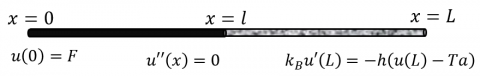
At the left end, a constant thermal source is assumed while the right end remains free allowing the process of convection. Figure 1 represents the stationary heat conduction problem.
Figure 1. Scheme for the mathematical model
This problem may be modeled by the following system of ordinary differential equations with boundary and continuity conditions:
$\left\{\begin{array}{rlr}u^{\prime \prime}(x) & =0, & 0<x<l \\ u^{\prime \prime}(x) & =0, & l<x<L, \\ u(0) & =F, & \\ u\left(l^{-}\right) & =u\left(l^{+}\right), & \\ \kappa_{A} u^{\prime}\left(l^{-}\right) & =\kappa_{B} u^{\prime}\left(l^{+}\right), & \\ \kappa_{B} u^{\prime}(L) & =-h\left(u(L)-T_{a}\right)\end{array}\right.$ (1)
where, u [℃] is the temperature of the bar, F [℃] is the value of the point source at x=0, $\kappa_{\mathrm{A}}$ and $\kappa_{\mathrm{B}}$ [W/m℃] are the thermal conductivity constants of the homogeneous materials of the bar (note that A is the material on the left and B is the material on the right), h [W/m2℃] is the convection heat transfer coefficient, Ta [℃] represents the room temperature, and
$u\left(l^{-}\right)=\lim _{x \rightarrow l^{-}} u(x), u\left(l^{+}\right)=\lim _{x \rightarrow l^{+}} u(x)$,
$u^{\prime}\left(l^{-}\right)=\lim _{x \rightarrow l^{-}} u^{\prime}(x), u^{\prime}\left(l^{+}\right)=\lim _{x \rightarrow l^{+}} u^{\prime}(x)$. (2)
The solution to the problem (1)-(2) is given by:
$u(x)= \begin{cases}F+\frac{\kappa_{B} h\left(T_{a}-F\right)}{\zeta} x, & 0 \leq x \leq l \\ F+\frac{h\left(T_{a}-F\right)\left(l\left(\kappa_{B}-\kappa_{A}\right)+\kappa_{A} x\right)}{\zeta}, & l<x \leq L\end{cases}$ (3)
where,
$\zeta=\kappa_{A} \kappa_{B}+\kappa_{A} h L+\left(\kappa_{B}-\kappa_{A}\right) h l .$ (4)
Details on the solution (3)-(4), its properties and examples, can be found in [15-17].
Without loss of generality, from now on it is assumed that F>Ta.
In this section, the inverse problem consisting in the estimation of the thermal conductivities of the material, is explained for two different situations. Analytical expressions for the thermal conductivities are obtained where the estimations depend on the available data for each case.
This is an inverse problem. To solve it, we first solve the forward problem, which consist in calculating the temperature along the bar when the materials are known. In order to solve the inverse problem, we compare the measurement of the temperature with the solution to the forward problem (which depends on the material properties). Then, we obtain the values for the materials’ conductivity.
3.1 Case 1: Estimation based on two temperature measurements
The first estimation procedure assumes that two noisy temperature measurements are given: one at the interface, denoted by T1, and the other one at the right edge of the bar, denoted as T2.
The analytical solution given in (3)-(4), to the forward problem (1)-(2), is evaluated at x=l and at x=L, this allows to obtain:
$\left\{\begin{array}{l}u(l)=F+\frac{\kappa_{B} h\left(T_{a}-F\right)}{\kappa_{A} \kappa_{B}+\kappa_{A} h L+\left(\kappa_{B}-\kappa_{A}\right) h l} l, \\ u(L)=F+\frac{h\left(T_{a}-F\right)\left(l\left(\kappa_{B}-\kappa_{A}\right)+\kappa_{A} L\right)}{\kappa_{A} \kappa_{B}+\kappa_{A} h L+\left(\kappa_{B}-\kappa_{A}\right) h l}.\end{array}\right.$ (5)
After some algebraic computation it results:
$\left\{\begin{array}{c}F-u(l)=\frac{\kappa_{B} h\left(F-T_{a}\right)}{\kappa_{A} \kappa_{B}+\kappa_{A} h L+\left(\kappa_{B}-\kappa_{A}\right) h l} l, \\ u(l)-u(L)=\frac{\kappa_{A} h\left(F-T_{a}\right)(L-l)}{\kappa_{A} \kappa_{B}+\kappa_{A} h L+\left(\kappa_{B}-\kappa_{A}\right) h l}.\end{array}\right.$ (6)
From the ratio between the expressions given in (6), the following relation between the thermal conductivities is obtained:
$\kappa_{B}=\frac{F-u(l)}{u(l)-u(L)} \frac{(L-l)}{l} \kappa_{A}$ (7)
Replacing Eq. (7) in the any of the equations given in (6), the thermal conductivities are obtained as nonlinear functions on the temperature at x=l and x=L as follows:
$\kappa_{A}=h l \frac{u(L)-T_{a}}{F-u(l)}$ (8)
$\kappa_{B}=h(L-l) \frac{u(L)-T_{a}}{u(l)-u(L)}$ (9)
Note a unique expression for each coefficient $\kappa_{A}$ and $\kappa_{B}$ are obtained from the nonlinear equations given in (6).
The measured temperatures at x=l and x=L, T1 and T2, respectively, yield the following estimates $\widehat{\kappa_{A}}, \widehat{\kappa_{B}}$, for the materials conductivities.
$\widehat{\kappa_{A}}=h l \frac{T_{2}-T_{a}}{F-T_{1}}$ (10)
$\widehat{\kappa_{B}}=h(L-l) \frac{T_{2}-T_{a}}{T_{1}-T_{2}}$ (11)
The necessary and sufficient conditions for the existence of the solution to the proposed inverse problem are given by:
$T_{a}<T_{2}<T_{1}<F$ (12)
3.2 Case 2: Estimation based on a temperature measurement and a heat flow measurement
The second estimation technique is based on a noisy temperature measurement data at the interface, T1 and a heat flux measurement, q1 at the right edge of the bar.
From the solution given in (3)-(4) it follows that the heat flux q at x=L is:
$q=-\kappa_{B} u^{\prime}(L)=\frac{-\kappa_{B} \kappa_{A} h\left(T_{a}-F\right)}{\kappa_{A} \kappa_{B}+\kappa_{A} h L+\left(\kappa_{B}-\kappa_{A}\right) h l}$ (13)
The ratio between (13) and the first equation in (6) lead to:
$\frac{q}{F-u(l)}=\frac{\kappa_{A}}{l}$ (14)
After some algebraic computations, using Eq. (14) in Eq. (13), the thermal conductivities are obtained as functions on the temperature at x=l and the heat flux at x=L as follows:
$\kappa_{A}=\frac{q l}{F-u(l)}$ (15)
$\kappa_{B}=\frac{h(L-l)}{\frac{h}{q}\left(u(l)-T_{a}\right)-1}$ (16)
Estimated values $\widehat{\kappa_{A}}, \widehat{\kappa_{B}}$ for $\kappa_{A}, \kappa_{B}$ are obtained by replacing u(l) and q by the measured data T1 and q1, respectively, leading to:
$\widehat{\kappa_{A}}=\frac{q_{1} l}{F-T_{1}}$ (17)
$\widehat{\kappa_{B}}=\frac{h(L-l)}{\frac{h}{q_{1}}\left(T_{1}-T_{a}\right)-1}$ (18)
The necessary and sufficient conditions for the existence of the solution to the inverse problem are given by:
$T_{a}<T_{1}<F$ (19)
and
$q_{1}<h\left(T_{1}-T_{a}\right)$ (20)
In this section we derive a bound for the error in estimating the thermal conductivities, depending on available data.
4.1 Error analysis for the Case 1
In this case, it is assumed that the errors of the measured temperatures T1, and T2, satisfy the following inequalities:
$\left\{\begin{array}{l}\left|u(l)-T_{1}\right|<\varepsilon\left(F-T_{a}\right), \\ \left|u(L)-T_{2}\right|<\varepsilon\left(F-T_{a}\right)\end{array}\right.$ (21)
where, the dimensionless constant $\varepsilon \in(0,1)$ depends on the error produced by the measurement tools, among others.
From the expressions for the thermal conductivities given in (8)-(11), it follows:
$\left|\kappa_{A}-\widehat{\kappa_{A}}\right|=h l\left|\frac{u(L)-T_{a}}{F-u(l)}-\frac{T_{2}-T_{a}}{F-T_{1}}\right|$ (22)
$\left|\kappa_{B}-\widehat{\kappa_{B}}\right|=h(L-l)\left|\frac{u(L)-T_{a}}{u(l)-u(L)}-\frac{T_{2}-T_{a}}{T_{1}-T_{2}}\right|$ (23)
Let us consider (22). Observe that
$\left|\frac{u(L)-T_{a}}{F-u(l)}-\frac{T_{2}-T_{a}}{F-T_{1}}\right|=\left|\frac{u(L) F-u(L) T_{1}+T_{a} T_{1}-T_{2} F+T_{2} u(l)-u(l) T_{a}}{(F-u(l))\left(F-T_{1}\right)} \quad \right|.$
After adding and subtracting T1T2 in the numerator, rearranging terms and performing some algebraic computations it results:
$\left|\frac{u(L)-T_{a}}{F-u(l)}-\frac{T_{2}-T_{a}}{F-T_{1}}\right|=\frac{\left|\left(u(L)-T_{2}\right)+\left(u(l)-T_{1}\right) \frac{T_{2}-T_{a}}{F-T_{1}}\right|}{|F-u(l)|}$ (24)
By using the triangular inequality and assuming that (12) and (21) hold, it follows that:
$\left|\frac{u(L)-T_{a}}{F-u(l)}-\frac{T_{2}-T_{a}}{F-T_{1}}\right| \leq \frac{\left|u(L)-T_{2}\right|+\left|u(l)-T_{1}\right| \frac{T_{2}-T_{a}}{F-T_{1}}}{F-u(l)}<\frac{1+\frac{T_{2}-T_{a}}{F-T_{1}}}{F-u(l)} \varepsilon\left(F-T_{a}\right)$ (25)
Observe that F > u(l) > Ta. Hence,
$0<F-u(l)<F-T_{a}$ (26)
and there exists a dimensionless constant $M_{1} \in(0,1)$ such that:
$M_{1}<\frac{F-u(l)}{F-T_{a}}$ (27)
hence, inequality (25) can be written as:
$\left|\frac{u(L)-T_{a}}{F-u(l)}-\frac{T_{2}-T_{a}}{F-T_{1}}\right|<\frac{1}{M_{1}}\left(1+\frac{T_{2}-T_{a}}{F-T_{1}}\right) \varepsilon$ (28)
Replacing (28) in (22) it turns out that:
$\left|\kappa_{A}-\widehat{\kappa_{A}}\right|<h l A_{1} \varepsilon$ (29)
where, the dimensionless constant A1 depends on the data measurements, T1,T2 and it is given by:
$A_{1}=\frac{1}{M_{1}}\left(1+\frac{T_{2}-T_{a}}{F-T_{1}}\right)$ (30)
Similarly, assuming that (12) and (21) hold, it is possible to write:
$\left|\kappa_{B}-\widehat{\kappa_{B}}\right|=h(L-l)$$\left|\frac{\left(T_{2}-T_{a}\right)\left(T_{1}-u(l)\right)+\left(T_{1}-T_{a}\right)\left(u(L)-T_{2}\right)}{(u(l)-u(L))\left(T_{1}-T_{2}\right)}\right|<h(L-l)\left(\frac{\left(T_{2}-T_{a}\right)+\left(T_{1}-T_{a}\right)}{u(l)-u(L)}\right)\left(\frac{F-T_{a}}{T_{1}-T_{2}}\right) \varepsilon$ (31)
Since F > u(l) > u(L) > Ta, the inequalities:
$0<u(l)-u(L)<F-T_{a}$ (32)
Hold and there exists a dimensionless constant $M_{2} \in(0,1)$ such that:
$M_{2}<\frac{u(l)-u(L)}{F-T_{a}}$ (33)
Therefore,
$\left|\kappa_{B}-\widehat{\kappa_{B}}\right|<\frac{h(L-l)}{M_{2}}\left(1+2 \frac{T_{2}-T_{a}}{T_{1}-T_{2}}\right) \varepsilon$ (34)
or, equivalently,
$\left|\kappa_{B}-\widehat{\kappa_{B}}\right|<h(L-l) B_{1} \varepsilon$ (35)
where, the dimensionless constant B1 depends on the data measurements, T1, T2 and it is given by:
$B_{1}=\frac{1}{M_{2}}\left(1+2 \frac{T_{2}-T_{a}}{T_{1}-T_{2}}\right)$ (36)
hence, the inequalities (29)-(30) and (35)-(36) imply that the estimation errors for $\kappa_{A}, \kappa_{B}$ vanish as the measurement error (or $\varepsilon$) approaches 0. The dimensionless constant A1 and B1 determine the “velocity” of the converges of the estimation errors to 0. In other words, the estimation errors vanish as the errors in data approaches 0, independently of the dimensionless constant, but if these constants are big, the data error should be small to have a good estimate for the conductivities.
4.2 Error analysis for the Case 2
In this case, it is assumed that the errors of the measured temperature T1, and the measured heat flux q1, satisfy the following inequalities:
$\left\{\begin{array}{l}\left|u(l)-T_{1}\right|<\varepsilon\left(F-T_{a}\right), \\ \left|q-q_{1}\right|<\varepsilon h\left(F-T_{a}\right).\end{array}\right.$ (37)
where, as before, the dimensionless constant $\varepsilon \in(0,1)$ depends on the error produced by the measurement tools, among others.
From the expressions for the thermal conductivities given in Eqns. (15)-(18), we can write:
$\left|\kappa_{A}-\widehat{\kappa_{A}}\right|=l\left|\frac{q_{1}}{F-T_{1}}-\frac{q}{F-u(l)}\right|$ (38)
and
$\left|\kappa_{B}-\widehat{\kappa_{B}}\right|=\left|\frac{h(L-l)}{\frac{h\left(T_{1}-T_{a}\right)}{q_{1}}-1}-\frac{h(L-l)}{\frac{h\left(u(l)-T_{a}\right)}{q}-1}\right|$ (39)
Let us consider Eq. (38), that is the error $\kappa_{A}$. Note that:
$\left|\frac{q_{1}}{F-T_{1}}-\frac{q}{F-u(l)}\right|=\left|\frac{F\left(q_{1}-q\right)-q_{1} u(l)+T_{1} q}{\left(F-T_{1}\right)(F-u(l))} \quad \right|$
or, equivalently, adding and subtracting T1q1 in the numerator, rearranging terms and using condition (19) and triangular inequality it results:
$\left|\frac{q_{1}}{F-T_{1}}-\frac{q}{F-u(l)}\right|=\left|\frac{\left(F-T_{1}\right)\left(q_{1}-q\right)+q_{1}\left(T_{1}-u(l)\right)}{\left(F-T_{1}\right)(F-u(l))} \quad \right| \leq \frac{\left(F-T_{1}\right)\left|q_{1}-q\right|+q_{1}\left|T_{1}-u(l)\right|}{\left(F-T_{1}\right)(F-u(l))}$.
Hence, by conditions (37), it follows that
$\left|\frac{q_{1}}{F-T_{1}}-\frac{q}{F-u(l)}\right|<\frac{\left(F-T_{1}\right) \varepsilon h\left(F-T_{a}\right)+\varepsilon q_{1}\left(F-T_{a}\right)}{\left(F-T_{1}\right)(F-u(l))}=\frac{\left(F-T_{1}\right) h+q_{1}}{F-u(l)} \varepsilon\left(\frac{F-T_{a}}{F-T_{1}}\right)$. (40)
Then, replacing inequality (40) in (38), it results:
$\left|\kappa_{A}-\widehat{\kappa_{A}}\right|<l\left(\frac{\left(F-T_{1}\right) h+q_{1}}{F-u(l)}\right) \varepsilon\left(\frac{F-T_{a}}{F-T_{1}}\right)$ (41)
From (19) and (27) it follows that:
$\left|\kappa_{A}-\widehat{\kappa_{A}}\right|<l\left(\frac{\left(F-T_{1}\right) h+q_{1}}{M_{1}}\right)\left(\frac{1}{F-T_{1}}\right) \varepsilon$ (42)
or, equivalently,
$\left|\kappa_{A}-\widehat{\kappa_{A}}\right|<h l A_{2} \varepsilon$ (43)
where, the dimensionless constant A2 depends on the data measurements, T1, q1 and it is given by:
$A_{2}=\frac{1}{M_{1}}\left(1+\frac{q_{1}}{\left(F-T_{1}\right) h}\right)$ (44)
Let us consider the expression (39). Algebraic computations allow to rewrite it as:
$\left|\kappa_{B}-\widehat{\kappa_{B}}\right|=h^{2}(L-l)\left|\frac{q_{1}\left(u(l)-T_{a}\right)-q\left(T_{1}-T_{a}\right)}{\left[h\left(T_{1}-T_{a}\right)-q_{1}\right]\left[h\left(u(l)-T_{a}\right)-q\right]} \quad \right|$ (45)
Notice that, by the boundary condition at x=L given in Eq. (1), the heat flux satisfies q=h(u(L)-Ta) and the estimation error for $\kappa_{B}$ given in (45) can also be written as:
$\left|\kappa_{B}-\widehat{\kappa_{B}}\right|=h^{2}(L-l)\left|\frac{q_{1}\left(u(l)-T_{a}\right)-q\left(T_{1}-T_{a}\right)}{\left[h\left(T_{1}-T_{a}\right)-q_{1}\right][h(u(l)-u(L))]} \quad \right|$ (46)
Let us focus on the last factor in Eq. (46). The numerator and denominator of this factor are treated separately. Firstly, a bound depending on the measurement errors given in (37) are obtained for the numerator, while a constant bound is derived for the denominator.
Adding and subtracting q1T1 to the numerator, rearranging terms, taking common factor and using the triangle inequality results,
$\left|q_{1}\left(u(l)-T_{a}\right)-q\left(T_{1}-T_{a}\right)\right|=\left|q_{1}\left(u(l)-T_{1}\right)-\left(q-q_{1}\right)\left(T_{1}-T_{a}\right)\right| \leq q_{1}\left|u(l)-T_{1}\right|+\left|q-q_{1}\right|\left(T_{1}-T_{a}\right)$
and conditions (37) yield
$\left|q_{1}\left(u(l)-T_{a}\right)-q\left(T_{1}-T_{a}\right)\right|<\left(q_{1}+h\left(T_{1}-T_{a}\right)\right)\left(F-T_{a}\right) \varepsilon$ (47)
A bound for the denominator in (46) is obtained by (33) since:
$\left|\left[h\left(T_{1}-T_{a}\right)-q_{1}\right][h(u(l)-u(L))]\right|>\left|h\left(T_{1}-T_{a}\right)-q_{1}\right| h M_{2}\left(F-T_{a}\right)$ (48)
Therefore, (46)-(48) along with condition (20) yield:
$\left|\kappa_{B}-\widehat{\kappa_{B}}\right|<h(L-l) \frac{1}{M_{2}} \frac{h\left(T_{1}-T_{a}\right)+q_{1}}{h\left(T_{1}-T_{a}\right)-q_{1}} \varepsilon$ (49)
or, equivalently,
$\left|\kappa_{B}-\widehat{\kappa_{B}}\right|<h(L-l) B_{2} \varepsilon$ (50)
where, the dimensionless constant B2 depends on the data measurements, T1, q1 and it is given by:
$B_{2}=\frac{1}{M_{2}}\left(1+2 \frac{q_{1}}{h\left(T_{1}-T_{a}\right)-q_{1}}\right)$ (51)
Hence, the inequalities (43)-(44) and (50)-(51) imply that the estimation errors for $\kappa_{A}, \kappa_{B}$ vanish as the measurement error (or ε) approaches 0. The dimensionless constant A2 and B2 determine the “velocity” of the converges of the estimation errors to 0. In other words, the estimation errors vanish as the errors in data approaches 0, independently of the dimensionless constant, but if these constants are big the data error should be small to have a good estimate for the conductivities.
Eqns. (10)-(11) and (17)-(18) indicate that the estimated values of thermal conductivities depend on the parameters of the problem and on data. There are some tools that help to study the influence of the data on the estimated parameters. Among them, the sensitivity [18, 19] and elasticity analysis [15, 17, 19] are frequently used in the literature. The latter is widely used in economics and provides the percentage of error in the estimation for an error of 1% in the measured data.
Letting p the parameter to be estimated and d the data, the elasticity function is defined by:
$E(d)=\frac{d}{p} \frac{\partial p}{\partial d}$ (52)
The inverse problem presented here, consists in the identification of two parameters, and each of them depends on two data, hence four elasticity functions are considered for each case of estimation presented, analyzed and formalized in Section 3.
5.1 Elasticity analysis for the Case 1
For this case, the identification is based on two temperature measurements, one at the interface, T1 and the other at the right edge, T2. The elasticity functions of each parameter to be estimated with respect to each temperature measurement are obtained from the Eqns. (10)-(11) using the formula given in Eq. (52). This process leads to the following four elasticity functions.
$E_{1}\left(T_{1}\right)=\frac{T_{1}}{\widehat{\kappa_{A}}} \frac{\partial \widehat{\kappa_{A}}}{\partial T_{1}} \Rightarrow E_{1}\left(T_{1}\right)=\frac{T_{1}}{F-T_{1}}$ (53)
$E_{2}\left(T_{2}\right)=\frac{T_{2}}{\widehat{\kappa_{A}}} \frac{\partial \widehat{\kappa}_{A}}{\partial T_{2}} \Rightarrow E_{2}\left(T_{2}\right)=\frac{T_{2}}{T_{2}-T_{a}}$ (54)
$E_{3}\left(T_{1}\right)=\frac{T_{1}}{\widehat{\kappa_{B}}} \frac{\partial \widehat{\kappa_{B}}}{\partial T_{1}} \Rightarrow E_{3}\left(T_{1}\right)=\frac{T_{1}}{T_{2}-T_{1}}$ (55)
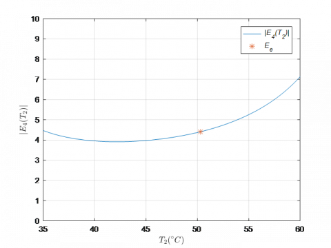
$E_{4}\left(T_{2}\right)=\frac{T_{2}}{\widehat{\kappa_{B}}} \frac{\partial \widehat{\kappa_{B}}}{\partial T_{2}} \Rightarrow E_{4}\left(T_{2}\right)=\frac{T_{2}\left(T_{1}-T_{a}\right)}{\left(T_{1}-T_{2}\right)\left(T_{2}-T_{a}\right)}$ (56)
Notice that E1 and E2 depend only on one of the temperature measurements, while E3 and E4 depend on both measurements. To analyzed E3 a fixed value for T2 is considered. Analogously, a fixed value of T1 is considered in order to analyzed the elastivity function E4.
5.2 Elasticity analysis for the Case 2
In this case, the identification is based on a temperature measurement at the interface, T1 and a thermal flow measurement at the right edge, q1. The elasticity functions are now obtained from Eqns. (17)-(18):
$E_{1}\left(T_{1}\right)=\frac{T_{1}}{\widehat{\kappa_{A}}} \frac{\partial \widehat{\kappa_{A}}}{\partial T_{1}} \Rightarrow E_{1}\left(T_{1}\right)=\frac{T_{1}}{F-T_{1}}$ (57)
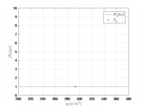
$E_{2}\left(q_{1}\right)=\frac{q_{1}}{\widehat{\kappa_{A}}} \frac{\partial \widehat{\kappa_{A}}}{\partial q_{1}} \Rightarrow E_{2}\left(q_{1}\right)=1$ (58)
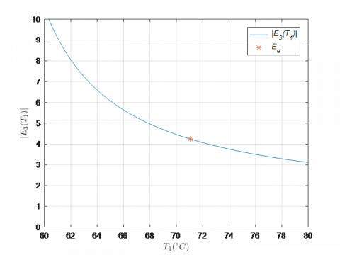
$E_{3}\left(T_{1}\right)=\frac{T_{1}}{\widehat{\kappa_{B}}} \frac{\partial \widehat{\kappa_{B}}}{\partial T_{1}} \Rightarrow E_{3}\left(T_{1}\right)=-\frac{T_{1}}{T_{1}-T_{a}-\frac{q_{1}}{h}}$ (59)
$E_{4}\left(q_{1}\right)=\frac{q_{1}}{\widehat{\kappa_{B}}} \frac{\partial \widehat{\kappa_{B}}}{\partial q_{1}} \Rightarrow E_{4}\left(q_{1}\right)=\frac{T_{1}-T_{a}}{T_{1}-T_{a}-\frac{q_{1}}{h}}$ (60)
It can be observed from (57)-(58) that the estimation of $\kappa_{A}$ does not depend on the value of q1. In particular, the percentage of error in the estimation of $\kappa_{A}$ is constant, equal to 1, regardless of the value of q1. On the other hand, the percentage error in the estimation of $\kappa_{B}$ depends on both measurements, as in the Case 1. Then, to analyzed E3, a fixed value for q1 is considered, while a fixed value of T1 is considered in order to analyzed the elasticity function E4.
In this section, the thermal conductivity is estimated numerically for each case descripted in Section 3, where data are calculated from the solution to the forward problem and random noise is added to simulate experimental measurements.
The inverse problem is solved considering the configuration described in Table 1 where the bar is assumed to be composed by Pb on the left (0 < x < l) and Fe on the right (l < x < L). The values for $\kappa_{A} \cdot \kappa_{B}$ are obtained from [16].
Table 1. Problem setup data
|
L |
l |
F |
Ta |
h [20] |
$\kappa_{A}$ |
$\kappa_{B}$ |
|
10m |
4m |
100℃ |
25℃ |
10W/m2℃ |
35W/m℃ |
73W/m℃ |
The thermal conductivity coefficients are estimated using Eqns. (10)-(11) or Eqns. (17)-(18) depending on the available data. For each case, a table is included to show the simulated data and the relative errors. Then, the absolute values of elasticity functions, given in Eqns. (53)-(56) or Eqns. (57)-(60), respectively, are plotted and the results are analyzed.
6.1 Numerical estimation for the case 1
The temperatures at the interface (x=l) and at the right edge (x=L) are given in Eq. (5). For this example, the values are u(l)=71.08℃ and u(L)=50.30℃.
Table 2. Relative estimation errors of $\kappa_{A}$ and $\kappa_{B}$
|
T1(°C) |
T2(°C) |
$\frac{\left|K_{A}-\widehat{K}_{A}\right|}{K_{A}}$ |
$\frac{\left|\kappa_{B}-\widehat{\kappa_{B}}\right|}{\kappa_{B}}$ |
|
70.5 |
49.8 |
0.0392 |
0.0152 |
|
70.6 |
49.9 |
0.0320 |
0.0113 |
|
70.7 |
50 |
0.0248 |
0.0073 |
|
70.8 |
50.1 |
0.0176 |
0.0033 |
|
70.9 |
50.2 |
0.0103 |
0.0005 |
|
71 |
50.3 |
0.0029 |
0.0044 |
|
71.1 |
50.4 |
0.0044 |
0.0085 |
|
71.2 |
50.5 |
0.0119 |
0.0125 |
|
71.3 |
50.6 |
0.0194 |
0.0164 |
Table 2 shows the relative errors for the estimated parameters considering different values of simulated data T1 and T2, in a neighborhood of the exact values u(l) and u(L), respectively. The results show that, the maximum errors for the values considered here, are about 4% in the estimation of $\kappa_{A}$ and 2% in the estimation of $\kappa_{B}$.
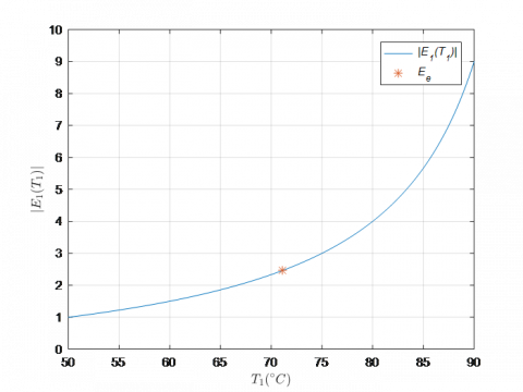
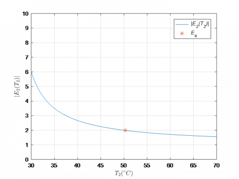
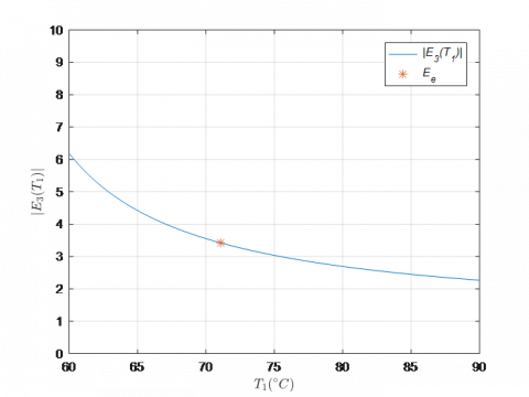
The absolute values of elasticity functions given by the expressions (53)-(56) are plotted in Figures 2-5.
The elasticity analysis shows that an error of 1% in the measurement of the temperature T1 implies an error of 2.5% in the estimation of $\kappa_{A}$ and of 3.5% in the estimation of $\kappa_{B}$. Furthermore, it is observed that an error of 1% in the measurement of the temperature T2 translates into an error in the estimation of $\kappa_{A}$ of 2% and of $\kappa_{B}$ of 4.5%.
Figure 2. Plot of |E1(T1)|: Absolute value of the elasticity of $\widehat{\kappa_{A}}$ with respect to T1
Figure 3. Plot of |E2(T2)|: Absolutve value of the elasticity of $\widehat{\kappa_{A}}$ with respect to T2
Figure 4. Plot of |E3(T1)|: Absolute value of the elasticity of $\widehat{\kappa_{B}}$ with respect to T1 (T2=50.30°C)
Figure 5. Plot of |E4(T2)|: Absolute value of the elasticity of $\widehat{\kappa_{B}}$ with respect to T2 (T1=71.08°C)
6.2 Numerical estimation for the case 2
The temperatures at the interface and the heat flux at the free edge are given in Eq. (5) and Eq. (13). Considering the values in Table 1, u(l)= 71.08℃ and q=292.97 W/m2.
Table 3 shows the relative errors obtained for the estimated parameters using different values of temperature T1 and q1 around the exact values of u(l) and q, respectively. The results show that, the maximum errors for the values considered here, are about 2% in the estimation of $\kappa_{A}$ and 4% in the estimation of $\kappa_{B}$.
Table 3. Relative estimation errors of $\kappa_{A}$ and $\kappa_{B}$
|
T1(°C) |
q1(W/m2) |
$\frac{\left|\kappa_{A}-\widehat{\kappa_{A}}\right|}{\kappa_{A}}$ |
$\frac{\left|\kappa_{B}-\widehat{\kappa_{B}}\right|}{\kappa_{B}}$ |
|
70.5 |
252.92 |
0.0201 |
0.0287 |
|
70.6 |
252.93 |
0.0167 |
0.0237 |
|
70.7 |
252.94 |
0.0134 |
0.0188 |
|
70.8 |
252.95 |
0.0099 |
0.0139 |
|
70.9 |
252.96 |
0.0065 |
0.0090 |
|
71 |
252.97 |
0.0030 |
0.0043 |
|
71.1 |
252.98 |
0.0004 |
0.0004 |
|
71.2 |
252.99 |
0.0039 |
0.0051 |
|
71.3 |
253.00 |
0.0074 |
0.0098 |
The absolute values of the elasticity functions given by the expression (57)-(60) are plotted below (Figures 6-9).
Figure 6. Plot of |E1(T1)|: Absolute value of the elasticity of $\widehat{\kappa_{A}}$ with respect to T1
Figure 7. Plot of |E2(q1)|: Absolute value of the elasticity of $\widehat{\kappa_{A}}$ with respect to q1
Figure 8. Plot of |E3(T1)|: Elasticity in absolute value of $\widehat{\kappa_{B}}$ with respect to T1 (q1=292.97 W/m2)
Figure 9. Plot of |E4(q1)|: Elasticity in absolute value of $\widehat{\kappa_{B}}$ with respect to q1 (T1=71.08℃)
The elasticity analysis, for this case, indicates that an error of 1% in the measurement of the temperature T1 implies an error of 2.5% in the estimation of $\kappa_{A}$ and of 4.2% in the estimation of $\kappa_{B}$. Furthermore, it is observed that an error of 1% in the measurement of the heat flux q1 produces an error of 1% in the estimation of $\kappa_{A}$ and about 2.8% for the estimation of $\kappa_{B}$.
It is considered a stationary heat transfer process in a bar made of two perfectly assembled sections of homogeneous and isotropic materials. A Dirichlet condition is assumed at the left boundary and a Robin type condition is assumed at the right one. The thermal conductivities of the materials are estimated based on two measurements. Firstly, two noisy temperature measurements, one at the interface and the other one at the right edge, are considered. Secondly, a noisy temperature measurement at the interface and a heat flow measurement at the right edge, are assumed.
The necessary and sufficient conditions are provided for the estimation of the parameters for each case. The bounds for the identification errors of the unknown coefficients are derived based on the data measurements, the room temperature and temperature values at the boundary and interface (the estimates are made from the data and the parameters of the direct problem). The error analysis makes clear that the identification is continuous with respect to data, in order words, they will vanish as the measurement errors approach zero; that is, the determination problem is a well-posed inverse problem.
An elasticity analysis is performed to study the local influence of the data on the estimated thermal conductivities and we show that the estimation errors are reasonable based on the simulated errors in the data.
The numerical examples presented here show a good performance in both cases and indicate that they could be useful to identify the materials in a bar involved in a similar heat transfer process.
The first and third authors acknowledge support from SOARD/AFOSR through grant FA9550-18-1-0523. The second author acknowledges support from European Union's Horizon 2020 Research and Innovation Programme under the Marie Sklodowska-Curie Grant Agreement No. 823731 CONMECH and by the Project PIP No. 0275 from CONICET-UA, Rosario, Argentina.
The authors appreciate the very useful comments made by the reviewer in order to improve this work.
|
A1 |
dimensionless auxiliary variable |
|
A2 |
dimensionless auxiliary variable |
|
B1 |
dimensionless auxiliary variable |
|
B2 |
dimensionless auxiliary variable |
|
d |
bar diameter, m |
|
E |
Elasticity |
|
F |
heat source, °C |
|
h |
convective coefficient, W.m-2.°C -1 |
|
L |
interface position, m |
|
L |
bar length, m |
|
q |
heat flow at the right edge, W. m-2 |
|
q1 |
measured heat flow at the right edge, W.m-2 |
|
M1 |
dimensionless auxiliary variable |
|
M2 |
dimensionless auxiliary variable |
|
T1 |
measured temperature at the interface, °C |
|
T2 |
measured temperature at the right edge, °C |
|
Ta |
room temperature, °C |
|
u |
temperature function on the bar, °C |
|
x |
spatial variable, m |
|
Greek symbols |
|
|
ε |
dimensionless measurement error |
|
${\kappa}$ |
thermal conductivity, W.m-1.°C -1 |
|
$\hat{\kappa}$ |
estimated thermal conductivity, W.m-1.°C -1 |
|
$\varsigma$ |
auxiliary variable, W2.m-2.°C -2 |
|
Subscripts |
|
|
A |
related to material A |
|
B |
related to material B |
|
e |
related to the exact value |
[1] Chung, D.D.L. (2001). Thermal interface materials. Journal of Materials Engineering and Performance, 10(1): 56-59. https://dx.doi.org/10.1361/105994901770345358
[2] Ma, H.Y., Zhu, P.X., Zhou, S.G., Xu, J., Huang, W.F., Yang, H.M., Chen, M.J. (2010). Preliminary research on Pb-Sn-Al laminated composite electrode materials Applied to zinc electrodeposition. Advanced Materials Research, 150: 303-308. https://dx.doi.org/10.4028/www.scientific.net/AMR.150-151.303
[3] Cahill, D.G., Ford, W.K., Goodson, K.E., Mahan, G.D., Majumdar, A., Maris, H.J., Merlin, R., Phiipot, S.R. (2003). Nanoscale thermal transport. Journal of Applied Physics, 93(2): 793-818. https://dx.doi.org/10.1063/1.1524305
[4] Clausing, A.M., Chao, B.T. (1965). Thermal contact resistance in a vacuum environment. Journal Heat Transfer, 87(2): 243-251. https://dx.doi.org/10.1115/1.3689082
[5] Barturkin, V. (2005). Micro-satellites thermal control-concepts and components. Acta Astronautica, 56(1-2): 161-170. https://doi.org/10.1016/j.actaastro.2004.09.003
[6] Flach. G.P., Özisik, M.N. (1989). Inverse heat conduction problem of simultaneously estimating spatially varying thermal conductivity and heat capacity per unit volume. Numerical Heat Transfer, Part A: Applications, 16(2): 249-266. https://dx.doi.org/10.1080/10407788908944716
[7] Lam, T.T., Yeung, W.K. (1995). Inverse determination of thermal conductivity for one-dimensional problems. Journal of Thermophysics and Heat Transfer, 9(2): 335-344. https://doi.org/10.2514/3.665
[8] Huang, C.H., Yan, J.Y., Chen, H.T. (1995). Function estimation in predicting temperature-dependent thermal conductivity without internal measurements. Journal of Thermophysics and Heat Transfer, 9(4): 667-673. https://doi.org/10.2514/3.722
[9] Yang, C.Y. (1998). A linear inverse model for the temperature-dependent thermal conductivity determination in one-dimensional problems. Applied Mathematical Modelling, 22(1): 1-9. https://doi.org/10.1016/S0307-904X(97)00101-7
[10] Yang, C.Y. (1999). Estimation of the temperature dependent thermal conductivity in inverse heat conduction problem. Applied Mathematical Modelling, 23(6): 469-478. https://doi.org/10.1016/S0307-904X(98)10093-8
[11] Salva, N.N., Tarzia, D.A. (2011). A sensitivity analysis for the determination of unknown thermal coefficients through a phase-change process with temperature-dependent thermal conductivity. International Communications in Heat and Mass Transfer, 38(4): 418-424. https://doi.org/10.1016/j.icheatmasstransfer.2010.12.017
[12] Tarzia, D.A. (1998). The determination of unknown thermal coefficients through phase change process with temperature-dependent thermal conductivity. International Communications in Heat and Mass Transfer, 25(1): 139-147. https://doi.org/10.1016/s0735-1933(97)00145-0
[13] Chantasiriwan, S. (2002). Steady-state determination of temperature-dependent thermal conductivity. International Communications in Heat and Mass Transfer, 29(6): 811-819. https://doi.org/10.1016/S0735-1933(02)00371-8
[14] Jurkowski, T., Jarny, Y., Delaunay, D. (1997). Estimation of thermal conductivity of thermoplastics under moulding conditions: An apparatus and an inverse algorithm. International Journal of Heat and Mass Transfer, 40(17): 4169-4181. https://doi.org/10.1016/s0017-9310(97)00027-6
[15] Umbricht, G.F., Rubio, D., Tarzia, D.A. (2020) Estimation technique for a contact point between two materials in a stationary heat transfer problem. Mathematical Modelling of Engineering Problems, 7(4): 607-613. https://doi.org/10.18280/mmep.070413
[16] Rubio, D., Tarzia, D.A., Umbricht, G.F. (2021). Heat transfer process with solid-solid interface: Analytical and numerical solutions. WSEAS Transactions on Mathematics, 20: 404-414. https://doi.org/10.37394/23206.2021.20.42
[17] Umbricht, G.F. Rubio, D., Tarzia, D.A. (2021). Estimation of a thermal conductivity in a stationary heat transfer problem with a solid-solid interface. International Journal of Heat and Technology, 39(2): 337-344. https://doi.org/10.18280/ijht.390202
[18] Banks, H.T., Dediu, S., Ernstberger, S.L. (2007). Sensitivity functions and their uses in inverse problems. Journal Inverse and Ill-posed Problems, 15: 683-708. https://dx.doi.org/10.1515/jiip.2007.038
[19] Sydsaeter, K., Hammond, P.J. (1995). Mathematics for Economic Analysis, Prentice Hall, New Jersey. ISBN 013583600X, 9780135836002
[20] Umbricht, G.F., Rubio, D., Echarri, R., El Hasi, C. (2020) A technique to estimate the transient coefficient of heat transfer by convection. Latin American Applied Research, 50(3): 229-234. https://doi.org/10.52292/j.laar.2020.179