Uma Ravi Sankar Yalavarthy* | Venkata Siva Krishna Rao Gadi
© 2022 IIETA. This article is published by IIETA and is licensed under the CC BY 4.0 license (http://creativecommons.org/licenses/by/4.0/).
OPEN ACCESS
This paper presents the design of an indirect space vector control (ISVC) of electric vehicle (EV) driven by permanent magnet synchronous motor (PMSM) utilizing the fuzzy logic control (FLC) approach for personnel transportation. Regulating the power flow in any vehicle is essential for optimal vehicle dynamics. A variety of propulsion motors are used in the system for such transmission. But PMSM is most efficient in terms of power density and torque. This study proposes a fuzzy controller based control technique for speed and torque control of PMSM drive and the simulated outcomes are compared with traditional PI controller under various motor loaded conditions. In this paper, EV dynamics are considered and ISVC strategy for PMSM is implemented. The PMSM is energized by space vector pulse width modulation (SVPWM) inverter. The system is modelled and simulated in MATLAB \ SIMULINK environment for steady speed-varying torque and varying speed-steady torque conditions. A wide range of speed drive profile is suggested for EV, consisting of accelerating, constant speed, decelerating, and rough road surface modes. Based on the results, the control technique was confirmed to be effective. The results indicate that the control scheme used is efficient throughout the wide range of speeds.
electric vehicle (EV), fuzzy logic controller (FLC), indirect space vector control (ISVC), permanent magnet synchronous motor (PMSM), space vector pulse width modulation (SVPWM)
In existing concerns of global warming, energy supply sustainability, and environmental impacts caused by the ever-increasing usage of internal combustion vehicles, EVs will be a necessary mode of personnel transportation. Because of its exceptional characteristics such as noiselessness, high efficiency, high torque, low losses in rotor, robustness owing to permanent magnets, high field weakening potentiality and high power density, PMSMs are frequently employed in electric vehicles [1-5].
Nonetheless, several experts and researchers have presented alternative techniques for EVs in selection of motor, inverter and control mechanism. The PMSM could be powered by sinusoidal PWM inverter, Z-source inverter and multilevel inverter [6, 7]. Due to less complexity in design and control mechanism SVPWM inverter is employed in this study and also the output voltage of SVPWM inverter is 15% greater relative to sinusoidal PWM inverter.
Many controllers such as predictive controller, hysteresis controller and adaptive controllers are developed and employed in the speed control of EVs [8-10]. Because of fewer complications in its operation and implementation fuzzy controller is utilised in this research. Fuzzy logic fundamental purpose is to develop easy adaptive and efficient regulation [11].
This study focuses on development of an indirect space vector control scheme and the implementation of fuzzy logic to regulate the speed and torque of an electric vehicle. The analysis mainly focused on modelling of EV and control mechanism [12-14].
The paper structure is, Section 2 contains all the EV dynamic modelling formulations. In Section 3 indirect space vector control scheme is to comprehend the operation of PMSM. Section 4 is discussed about fuzzy logic controller. Finally in section 5, the simulation results of various driving circumstances are displayed and followed by conclusion in section 6 at last.
There is a mass-power relationship that must be met by internal combustion engine vehicles, and this relationship must be met by EVs as well. As a result, for the development and evaluation of an EV to establish the size of motor, energy capacity, as well as any other system components. Firstly, net tractive effort must be computed [15, 16].
2.1 Tractive effort
Consider a vehicle of mass of Mu (kg) with vehicle speed of U (m.s-1) as depicted in table 1. The vehicle's acceleration can be written as:
$\frac{d U}{d t}=\frac{\Sigma F_{t}-\Sigma F_{r}}{\delta M_{u}}$ (1)
where total tractive effort is $\sum \mathrm{F}_{\mathrm{t}}$, total resistance is $\sum \mathrm{F}_{1}$, and δ is mass factor. The following is an expanded version of the aforementioned equation is given in Eq. (2).
$M_{u} \frac{d U}{d t}=\left(F_{t f}+F_{t r}\right)-\left(F_{r f}+F_{r r}+F_{w}+F_{g}\right)$ (2)
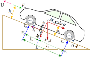
The tractive effort $\left(F_{t f}+F_{t r}\right)(N)$ on both tyres should be greater for the vehicle to accelerate. Acceleration of vehicle is achieved, when the net force imposed on body is not more than the tractive effort generated. The opposing forces comprise of rolling resistance on fore and rear tires $F_{r f}$ and $F_{r r}$ respectively, aerodynamic drag $F_{w}$ and grading resistance $F_{g}$. The friction between tyre and the road surface is known as rolling resistance, given in Eq. (3).
$F_{r}=P f_{r} \cos \alpha$ (3)
Figure 1. Acting forces on the vehicle moving uphill
Here, Coefficient of rolling resistance $f_{r}$ is approximately 0.01 for EV, which depends upon tyre’s material, structure, pressure and temperature, and also on liquid on the road surface. P is the load acting normally to surface.
Aerodynamic drag is the force exerted on a vehicle by air attempting to stop it from moving. Skin friction and shape drag and are the two basic components of this resistive force. This force depends upon air density $\rho\left(\mathrm{kg} \cdot \mathrm{m}^{-3}\right)$, front area of the vehicle $A_{f}\left(\mathrm{~m}^{2}\right)$.
$F_{w}=\frac{1}{2} \rho C_{d} A_{f}\left(U+U_{w}\right)^{2}$ (4)
where, $C_{d}$ is drag coefficient, which can be reduced by smart vehicle design. $U_{w}$ is the wind speed direction in relation to the direction of vehicle movement, with a negative sign when the vehicle travel in the same way and vice versa. The force for climbing the hill is given by:
$F_{g}=M_{U} g \sin \alpha$ (5)
For movement, total tractive force required is given by:
$F_{t}=F_{t f}+F_{t r}$ (6)
The net force generated by the vehicle's rear and front wheels is given by:
$\left.\begin{array}{rl}F_{t_{\max }} & =\frac{\mu M_{u} g \cos \alpha\left[L_{a}+f_{r}\left(h_{g}-r_{d}\right)\right] / L}{1+\mu h_{g} / L} \\ F_{t_{\max }} & =\frac{\mu M_{u} g \cos \alpha\left[L_{b}+f_{r}\left(h_{g}-r_{d}\right)\right] / L}{1+\mu h_{g} / L}\end{array}\right\}$ (7)
where, L is wheel base (m), hg is height of vehicle from its centre of gravity (m). For the vehicle to operate safely, the vehicle's power drive must not transcend the above mentioned limits. Otherwise, the tyres may whirl and the vehicle's functioning may become unstable. The load torque and reference angular speed on the machine could be transmitted from vehicle via power-train and gearbox as:
$\left.\begin{array}{c}T_{L}=\frac{r_{d}}{i_{g} i_{o} \eta_{t}}\left(F_{r}+F_{w}+M_{u} g \sin \alpha\right) \\ \omega_{r}^{*}=\frac{30 i_{g} i_{o} U_{r e f}}{\pi r_{d}}\end{array}\right\}$ (8)
where, $U_{r e f}$ is driver speed reference, $i_{g}$ is transmission gear ratio, $i_{o}$ is final drive gear ratio, $\mathrm{r}_{\mathrm{d}}$ is tyre effective radius (m), $\eta_{t}$ is efficiency of drive and $\mathrm{T}_{\mathrm{L}}$ is load torque (N.m).
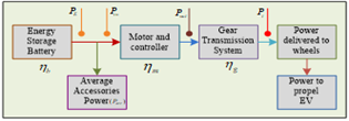
2.2 Power flow in electric vehicle
Figure 2 depicts the EV power flow. The power necessary to propel the EV for every second is computed for the entire drive period to predict the range. The procedure is continued up to the battery is fully exhausted. As a result, the power requirements must be calculated:
$P_{t}=F_{t} U$ (9)
The previous calculation of the tractive effort $F_{t}$ given in Eq. (7) is required for analysis of power flow. The efficiencies of gear mechanism, propulsion motor and storage system is considered. The efficiency of the controller and motor are regarded for our convenience. The efficiency of a motor greatly depends on its power, torque, and size. The equation accurately models the efficiency. Pin and Pout are the traction motor and controller's input and output power, respectively (W).
$\left.\begin{array}{c}\eta_{m}=\frac{P_{o u t}}{P_{i n}}=\frac{P_{o u t}}{P_{o u t}+\text { losses }} \\ \eta_{m}=\frac{T \omega}{T \omega+k_{c} T^{2}+k_{i} \omega+k_{W} \omega^{2}+C}\end{array}\right\}$ (10)
$k_{c}, k_{i}$ and $k_{w}$ are coefficients of copper, iron and windage losses respectively. $\mathrm{C}$ denotes the constant losses. Knowing the efficiency of motor $\left(\eta_{m}\right)$, input power and output power of the motor in driving and slowing conditions can be calculated. Eq. (11) is the case EV operating in driving mode.
$\left.\begin{array}{l}P_{\text {in }}=\frac{P_{\text {out }}}{\eta_{m}} \\ P_{\text {out }}=\frac{P_{t}}{\eta_{g}}\end{array}\right\}$ (11)
Figure 2. Power flow in electric vehicle
Eq. (12) is the case of decelerating or reaching rest mode in operating EV.
$\left.\begin{array}{c}P_{\text {in }}=P_{\text {out }} * \eta_{m} \\ P_{\text {out }}=P_{t} * \eta_{g}\end{array}\right\}$ (12)
Power drawn by energy storage battery is given by:
$P_{E}=P_{i n}+P_{a c c}$ (13)
In decelerating and braking mode of operating mode of operating EV, energy is fed back to energy storage unit by regenerative braking. The power flow block is modelled and simulated under accelerating, decelerating and constant speed modes.
3.1 PMSM d-q analysis
The dynamic mathematical model of PMSM is a multivariable, non-linear, higher order system. In most studies, the assumptions are made as follows:
(1) In the air gap, the magneto motive force has a sinusoidal distribution. (2) Neglecting iron losses and saturation of magnetic circuit. (3) Neglecting the effect of temperature and frequency variations on winding resistance. (4) Neglecting spatial harmonics. (5) Symmetrical distribution of three-phase windings. Dynamic mathematical model of PMSM is formulated under the following assumptions.
Analysing and solving of synchronous motor is difficult in static coordinate system as they have a collection of non-linear equations. So, in a synchronous rotating coordinate system, the mathematical model of PMSM in accord to vector transformation theory can be described by the following equations. The flux linkages between stator d-axis and q-axis windings are given in Eq. (14) [17, 18].
$\left.\begin{array}{c}\psi_{s d}=L_{s} i_{s d}+\psi_{f d} \\ \psi_{s q}=L_{s} i_{s q} \\ \text { where } L_{s}=L_{l s}+L_{m}\end{array}\right\}$ (14)
where, $L_{s}, L_{m}$ and $L_{l s}$ are stator self, mutual, stator leakage inductances $(\mathrm{H})$ respectively, $\psi_{s d}$ and $\psi_{s q}$ are d- axis and qaxis stator flux linkage (A.T) respectively, $i_{\text {sd }}$ is stator d-axis current (A), $\psi_{f d}$ is the stator d-axis winding flux linkage owing to flux produced by the permanent magnets of rotor. Note that d-axis is lined up to magnetic axis of rotor. Stator dq winding voltages of stator is given by:
$\left.\begin{array}{c}v_{s d}=R_{s} i_{s d}+\frac{d}{d t} \psi_{s d}-\omega_{m} \psi_{s q} \\ v_{s q}=R_{s} i_{s q}+\frac{d}{d t} \psi_{s q}+\omega_{m} \psi_{s d} \\ \omega_{m}=\frac{p}{2} \omega_{m e c h}\end{array}\right\}$ (15)
where, $v_{s d}, v_{s q}, i_{s d}, i_{s q}, R_{s}, \omega_{m}$ and $\omega_{\text {mech }}$ are d-axis stator voltage $(\mathrm{V})$, q-axis stator voltage (V), d-axis stator current (A), q-axis rotor current $(A)$, stator winding resistance $(\Omega)$, instantaneous speed of $\mathrm{d}-\mathrm{q}$ winding (electrical rad. $\mathrm{s}^{-1}$ ) and mechanical speed (mechanical rad. $\mathrm{s}^{-1}$ ) respectively. Electromagnetic torque $\mathrm{T}_{\mathrm{EM}}$ (N.m) produced is given by:
$T_{E M}=\frac{p}{2}\left(\psi_{s d} i_{s q}-\psi_{s q} i_{s d}\right)$ (16)
On substitution of Eq. (14) in Eq. (16), for non-salient pole machine,
$T_{E M}=\frac{p}{2}\left[\left(L_{s} i_{s d}+\psi_{f d}\right) i_{s q}-L_{s} i_{s q} i_{s d}\right]=\frac{p}{2} \psi_{f d} i_{s q}$ (17)
The electro dynamic acceleration of PMSM is the difference between the electromagnetic torque and total load torque acting on cumulative inertia of motor and load, J (kg.m2).
$\frac{d}{d t} \omega_{\text {mech }}=\frac{T_{E M}-T_{L}}{J}$ (18)
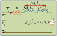
3.2 Relationship between d-q circuits and per phase equivalent circuit in steady-state
Figure 3. Steady-state per phase equivalent circuit
In analysis of PMSM, the two d-axis and q-axis winding equivalent circuits integrate to form the per phase equivalent circuit under balanced sinusoidal steady state condition shown in Figure 3. Under this condition, the d-q winding quantities are DC and the derivatives with respect to time are zero. Substituting flux connections from Eq. (14) for stator voltages in Eq. (15) results in:
$\mathrm{v}_{\mathrm{sd}}=\mathrm{R}_{\mathrm{s}} \mathrm{i}_{\mathrm{sd}}-\omega_{\mathrm{m}} \mathrm{L}_{\mathrm{s}} \mathrm{i}_{\mathrm{sq}}$ (19.1)
$\mathrm{v}_{\mathrm{sq}}=\mathrm{R}_{\mathrm{s}} \dot{\mathrm{i}}_{\mathrm{sq}}+\omega_{\mathrm{m}} \mathrm{L}_{\mathrm{s}} \dot{i}_{\mathrm{sd}}+\omega_{\mathrm{m}} \psi_{\mathrm{fd}}$ (19.2)
Multiplying both sides of Eq. (19.2) with j operator and adding to Eq. (19.1). Then multiplying the resultant equation by $\sqrt{3 / 2}$ results in:
$\vec{v}_{s}=R_{s} \vec{l}_{s}+j \omega_{m} L_{s} \vec{\imath}_{s}+\underbrace{j \sqrt{\frac{3}{2} \omega_{m} \psi_{f d}}}_{\vec{e}_{f s}}$ (20)
For other quantities, consider $\vec{v}_{s}=\sqrt{\frac{3}{2}}\left(v_{s d}+j v_{s q}\right)$ and so on. Under balanced steady state conditions, phase-a stator equation is given by $\mathrm{v}_{\mathrm{a}}=(3 / 2) \mathrm{v}_{\mathrm{s}}$, shown in Eq. (21).
$\bar{V}_{a}=R_{s} \bar{I}_{a}+j \omega_{m} L_{s} \bar{I}_{a}+\underbrace{j \sqrt{\frac{2}{3} \omega_{m} \psi_{f d}}}_{\bar{E}_{f a}}$ (21)
$\hat{E}_{f a}=\underbrace{\sqrt{\frac{3}{2} \psi_{f d}} \omega_{m}}_{K_{E}}=K_{E} \omega_{m}$ (22)
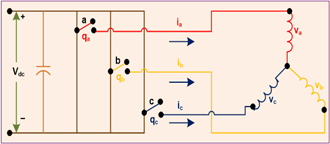
3.3 Design of SVPWM power processing unit (PPU)
SVPWM is mostly utilised in vector-controlled drives. The stator winding is connected in star, and assume negative of DC and hypothetical neutral of stator as reference ground, as illustrated in Figure 4 [17, 19-21]. At any instant, space vector stator voltage is written as:
$\overrightarrow{v_{s}^{a}(t)}=V_{d c}\left(q_{a}(t) e^{j 0}+q_{b}(t) e^{\frac{j 2 \pi}{3}}+q_{c}(t) e^{\frac{j 4 \pi}{3}}\right)$ (23)
Consider for pole-a, $q_{a}$ is logic 1 if the switch is in the up position otherwise 0 . Accordingly, we assign $1^{\prime}$ s and 0 's to $q_{b}$ and $q_{c}$ that correspond to pole-b and pole-c, respectively. Now, there are eight possible combinations of the $q_{c}, q_{b}$ and $q_{a}$ pattern 3-bit digital model. While we substitute all of the possible combinations in Eq. (23), Superscript a represents reference a-axis in three phase winding abc model. We get eight stator space vectors ranging from $\overrightarrow{v_{0}}$ to $\overrightarrow{v_{7}} \cdot \overrightarrow{v_{0}}, \overrightarrow{v_{7}}$ are treated as zero vectors, while $\overrightarrow{v_{1}}$ to $\overrightarrow{v_{6}}$ are treated as basic vectors.
Figure 4. SVPWM power processing unit internal circuit
At any instant, space vector stator voltage is written as:
$\overrightarrow{v_{s}^{a}(t)}=V_{d c}\left(q_{a}(t) e^{j 0}+q_{b}(t) e^{\frac{j 2 \pi}{3}}+q_{c}(t) e^{\frac{j 4 \pi}{3}}\right)$ (24)
The fundamental goal of this technique is to generate stator output phase voltages that are proportional to reference signals.
Figure 5. Six basic voltage space vectors representation
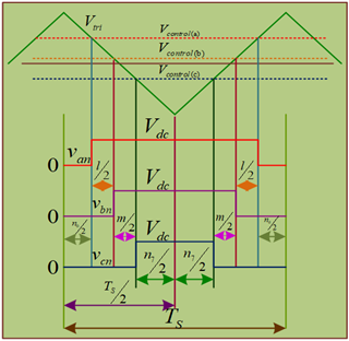
In order for SVPWM to achieve a constant switching frequency and the optimum harmonic response, each pole must only change its state once in each switching interval. For instance consider sector-I. In Figure $5, \overrightarrow{v_{1}}$ and $\overrightarrow{v_{3}}$ are applied for time intervals of $\mathrm{IT}_{\mathrm{s}}$ and $\mathrm{mT}_{\mathrm{s}}$, respectively, over a switching period $\mathrm{T}_{\mathrm{s}} . \overrightarrow{v_{0}}$ and $\overrightarrow{v_{7}}$ are the zero vectors applied for $\mathrm{n}_{0} \mathrm{~T}_{\mathrm{s}}$ and $\mathrm{n}_{7} \mathrm{~T}_{\mathrm{s}}$ respectively. Where $\mathrm{n}=\mathrm{n}_{0}+\mathrm{n}_{7}$, and $\mathrm{l}+\mathrm{m}+\mathrm{n}=$ 1. The stator vector voltage with reference a-axis is given by:
$\left.\begin{array}{c}\overrightarrow{v_{s}^{a}}=\frac{1}{T_{s}}\left(l T_{s} \overrightarrow{v_{1}}+m T_{s} \overrightarrow{v_{3}}+n T_{s}, 0\right) \\ \overrightarrow{v_{s}^{a}}=l \overrightarrow{v_{1}}+m \overrightarrow{v_{3}} \\ \Rightarrow \hat{V}_{s} e^{j \theta_{s}}=l V_{d c} e^{j 0}+m V_{d c} e^{\frac{j \pi}{3}}\end{array}\right\}$ (25)
Figure 6. Sector-I pole voltages over time period (Ts)
In Figure 6, pole-a have the longest time interval for the 'up' position, followed by pole-b, and finally pole-c. Thus switching can be done for any other sectors. The comparison of control voltages with the reference triangular voltage signal $\widehat{V}_{t r i}$ is included in the generation of the stator output voltage vector $\overrightarrow{v_{s}^{a}}$ with phase voltages $v_{a}, v_{b}$ and $v_{c}$ for specified $V_{d c}$ given in Eq. (26) The stator winding in PMSM is star connected to with isolated neutral. As a result, $v_{a}(t)+v_{b}(t)+v_{c}(t)=0$.
$\frac{\mathrm{V}_{\text {control }(\mathrm{a})}}{\hat{\mathrm{v}}_{\text {tri }}}=\frac{\mathrm{v}_{\mathrm{a}}-\mathrm{v}_{\mathrm{k}}}{\left(\mathrm{V}_{\mathrm{dc} / 2} \quad \right )} \quad$;
$\frac{\mathrm{V}_{\text {control }(\mathrm{b})}}{\hat{\mathrm{v}}_{\text {tri }}}=\frac{\mathrm{v}_{\mathrm{b}}-\mathrm{v}_{\mathrm{k}}}{\left(\mathrm{v}_{\mathrm{dc} / 2 \quad)}\right.} \quad$;
$\frac{\mathrm{V}_{\text {control }(\mathrm{c})}}{\hat{\mathrm{v}}_{\text {tri }}}=\frac{\mathrm{v}_{\mathrm{c}}-\mathrm{v}_{\mathrm{k}}}{\left(\mathrm{V}_{\mathrm{dc} / 2} \quad \right )} \quad$.
where $\mathrm{v}_{\mathrm{k}}=\frac{\max \left(\mathrm{v}_{\mathrm{a}}, \mathrm{v}_{\mathrm{b}}, \mathrm{v}_{\mathrm{c}}\right)+\min \left(\mathrm{v}_{\mathrm{a}}, \mathrm{v}_{\mathrm{b}}, \mathrm{v}_{\mathrm{c}}\right)}{2}$ (26)
Join the extreme points of the basic vectors to build a hexagon to set up the highest magnitude in output voltage of stator voltage space vector $\overrightarrow{V_{s}^{a}}$. The maximum value is given in Eq. (27).
Figure 7. Indirect space vector control of PMSM fed electric vehicle schematic
$\left|\overrightarrow{v_{s(\max )}^{a}} \quad \right|_{p h}=\frac{2}{3} V_{d c} \cos \left(\frac{\pi}{3}\right)=\frac{1}{\sqrt{3}} V_{d c}$
$\left|\overrightarrow{v_{s(m a x)}^{a}} \quad \right|_{L-L(r m s)}=$$\sqrt{3} \frac{\left|\overrightarrow{v_{s(m a x)}^{a}} \quad \right|_{p h}}{\sqrt{2}}=$$\frac{V_{d c}}{\sqrt{2}}=0.707 V_{d c}$ (27)
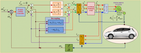
3.4 PMSM drive with a d-q based dynamic controller
A hysteretic converter was usually used in the absence of a dq analysis, with a non-constant switching frequency. Here SVPWM inversion control scheme is implemented, where the switching frequency remains constant for low speed and medium speed operations. For high speed propulsion of vehicle, the switching frequency of SVPWM inverter does not remains constant. To minimise harmonics in the speed profile, a low-pass filter is installed in series with the SVPWM power converter unit. Such control system schematic is shown in Figure 7. In Eq. (15), utilising the flux linkages of Eq. (14) and considering that the derivative of the rotor flux produced $\psi_{\mathrm{fd}}$ is zero; the voltages can be stated in the follows:
$\left.\begin{array}{c}v_{s d}=R_{s} i_{s d}+\frac{d}{d t} \psi_{s d}+\underbrace{-\omega_{m} L_{s} i_{s q}}_{\operatorname{comp}_{d}} \\ v_{s q}=R_{s} i_{s q}+\frac{d}{d t} \psi_{s q}+\underbrace{\omega_{m}\left(L_{s} i_{s d}+\psi_{f d}\right)}_{\operatorname{comp}_{q}}\end{array}\right\}$ (28)
In Figure 7, considering SVPWM PPU and utilising the decoupling compensation terms in Eq. (28) in d and q channels, PI controllers are being developed. The system is modeled in Simulink.
Figure 8. Fuzzy logic control functional block diagram
Figure 9. Fuzzy logic control interior organisation
The process flow diagram of FLC based control system is depicted in Figure 8 . The error in speed is the primary input $e_{\omega}$ and the variation of error in speed is secondary input $c e_{\omega}$, at sampling time $t_{s}$. At each sampling time, the two input variables $e_{\omega}$ and $c e_{\omega}$ are calculated and $c i_{s q}^{*}$ will be output. Here c denotes error or change. The $c i_{s q}^{*}$ signal is then sent to an integrator to acquire q-axis stator current for necessary speed control mechanism. The signal is then sent to ISVC SVPWM power processing unit to generate the required voltages to feed the PMSM drive for propulsion of EV. Thus the control strategy was implemented.
$e_{\omega}=\omega_{r e f}^{*}-\omega_{m}$
$c e_{\omega}=\frac{d}{d t}(e)$ (29)
where, $c e_{\omega}$ represents the error changes, $\omega_{\text {ref }}^{*}$ represents the reference rotor speed $\left(\mathrm{rad} . \mathrm{s}^{-1}\right), \omega_{m}$ represents the actual speed $\left(\operatorname{rad} . \mathrm{s}^{-1}\right)$.
FLC is proposed in particular a control hypothesis for the control approach of PMSM. Fuzzy control is straightforward and easy to implement; it is appropriate for nonlinear networks with varying and parametric change. FLC was developed and used to attain an acceptable rising and settling time periods, steady state error and overshoot. The suggested scheme reduces the reference PMSM speed variation. Fuzzy logic has a benefit above other control strategies in that it is not affected by changes in operational parameters. A PI controller controls the PMSM speed in the traditional space vector technique [22]. The suggested plan is to use a FLC instead of a traditional controller.
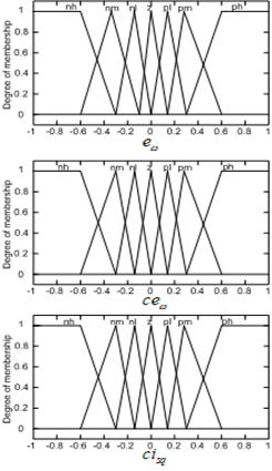
The fuzzy logic controller, as shown in Figure 9, has three phases: fuzzification, inference, and defuzzification [23, 24]. The primary input signal and its change for very small interval were processed into fuzzy numeral in the fuzzification block before being sent to the FLC. The fuzzy numeral of the calibrated output signal was therefore determined using the rule base. Lastly, the crisp values are transformed from the resultant integrated fuzzy subsets providing the controller output in defuzzification block [25, 26].
4.1 Fuzzification
Figure 10. Fuzzy controller membership functions
At this stage utilizing triangular membership functions, the variables of input $e_{\omega}$ and $c e_{\omega}$ which are crisp in nature, are converted to fuzzy variables $E_{\omega}$ and $C E_{\omega}$ as depicted in Figure 10. The input fuzzy variables $E_{\omega}$ and $C E_{\omega}$ have discourse universes of $[-12,12]$ and $[-1.4,1.4]$ respectively. On other hand, the output variable $\mathrm{Cl}_{\mathrm{sq}}^{*}$ have discourse universe of $[-10$, 10]. To make things easier, the entire discourse universe is normalized to $[-1,1]$.
The following linguistic labels are used by the proposed controller: nh, nm, nl, z, pl, pm and ph. All seven linguistics have a membership function for each input and output. Each fuzzy variable belongs to one of the data groups, for μ ranging from zero to one. μ is referred as membership degree. Basically, fuzzy logic is a type of artificial intelligence depending upon linguistic rules and knowledge. The following format is used to write these rules.
If i is L AND j is M… then k is N, where L, M and N represent membership functions, L and M are input fuzzy sets and N is output fuzzy set in above rule.
4.2 Inference stage
A matrix fuzzy relationship is established in this stage to determine the output of controller from the measured system variables. The matrix shows how fuzzy set characterising controller inputs and fuzzy set characterising controller outputs are related. As illustrated in Table 1, the inference engine processes the fuzzy variables $E_{\omega}$ and $C E_{\omega}$ that carries out a set of programming rules from a rule base (7x7). These seven inputs and output fuzzy sets were selected to provide an ability to adapt during choice inference. Control rules are developed based on knowledge of PMSM behaviour and occurrence.
Every rule is instructed in the format shown in the example below. IF $\left(E_{\omega}\right.$ is pm) AND $\left(C E_{\omega}\right.$ is nh) $\operatorname{THEN}\left(C I_{s q}^{*}\right.$ is nl). Various inference algorithms are used to generate $C I_{s q}^{*}$. This work uses the algorithm based on maximum and minimum inference, and the membership degree of $C I_{s q}^{*}$ is given in Eq. (30).
$\mu\left[\left(C I_{s q}^{*}\right)_{k}\right]=\max \left[\min \left\{\mu\left(E_{\omega_{i}}\right), \mu\left(C E_{\omega_{j}}\right)\right\}\right]$
for $1 \leq i \leq n, 1 \leq j \leq n$ (30)
Table 1. Rule base fuzzy control
|
$e_{\omega}$ $c e_{\omega}$ |
nh |
nm |
nl |
z |
pl |
pm |
ph |
|
nh |
nh |
nh |
nh |
nh |
nm |
nl |
z |
|
nm |
nh |
nh |
nh |
nm |
nl |
z |
pl |
|
nl |
nh |
nh |
nm |
nl |
z |
pl |
pm |
|
z |
nh |
nm |
nl |
z |
pl |
pm |
ph |
|
pl |
nm |
nl |
z |
pl |
pm |
ph |
ph |
|
pm |
nl |
z |
pl |
pm |
ph |
ph |
ph |
|
ph |
z |
pl |
pm |
ph |
ph |
ph |
ph |
|
nh=negative high |
nm=negative medium |
nl=negative low |
z=nearly zero |
||||
|
pl=positive low |
pm=positive medium |
p=positive high |
|
||||
4.3 Defuzzification
In this stage, the inference output variable $C I_{s q}^{*}$ is reconverted into a crisp value $c i_{s q}^{*}$. Many defuzzification algorithms were suggested in various literatures. In this case, an algorithm based on Mamdani centroid defuzzification is used, and the crisp value is determined by centre of gravity of the $C I_{s q}^{*}$ membership function given in Eq. (31).
$c i_{s q}^{*}=\frac{\int \mu\left(C I_{s q}^{*}\right) C I_{s q}^{*} d C I_{s q}^{*}}{\mu\left(C I_{s q}^{*}\right) d C I_{s q}^{*}}$ (31)
Integrating $C i_{s q}^{*}$ renders the vector control system's reference current $i_{s q}^{*}$ given in Eq. (32).
$i_{s q}^{*}=\int c i_{s q}^{*} d t$ (32)
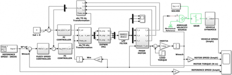
To accomplish simulation results, MATLAB / Simulink software is employed. To alleviate the PI controller's shortcomings, we suggested a cascaded FLC-based vector control in this study. The FLC provides a quick response in terms of low start-up current and quick response in attaining steady-state response. The indirect vector in rotor flux frame of reference control method based PMSM powered electric vehicle is developed and investigated in MATLAB / Simulink environment using Simulink library blocks. Figure 7 shows the architecture of PMSM fed by SVPWM power processing unit with a cascaded fuzzy controller. The system is modelled in Simulink is shown in Figure 11. In the d and q channels, the proportional constant Kp and integral constant Ki are 8.127 and 6.769e+03, respectively. The system is tested for both variable torque and variable speed profiles. A wide range speed command drive curve was of selected under various operating scenarios such as stair-case, step, trapezoidal and rough surfaces, the speed responses were observed.
The machine specifications influence the implementation of indirect vector control mechanism. The control block parameters are determined using the specifications in Table 2 and Section 4. Electric vehicle specifications are given in Table 3.
Table 2. PMSM and SVPWM inverter parameters study
|
Parameter, Symbol |
Value (dimension) |
|
Rated Voltage |
200 V |
|
Rated Current |
31.6 A |
|
Number of poles |
4 |
|
Rated frequency, f |
60 Hz |
|
Rated Speed |
6000 RPM |
|
Peak Torque, $T_{p e a k}$ |
12.9 N.m |
|
Rated Torque, $T_{\text {rated }}$ |
3.25 N.m |
|
Stator Resistance, $R_{s}$ |
0.145 Ω |
|
Stator Inductance, $L_{S}$ |
1.366 mH |
|
Total Inertia, J |
0.34x10⁻³ kg.m2 |
|
Voltage Constant, $K_{E}$ |
0.0958 V/(elec.rad.s-1) |
|
Battery Voltage, $V_{d c}$ |
300 V |
|
Reference triangular voltage, $V_{t r i}$ |
5 V |
|
Switching Frequency, $f_{s w}$ |
10 kHz |
In terms of implementation approach, the stator d-axis quadrature current is kept at its rated value $i_{d s}=0$, thus dcomponent of stator current is open looped. The stator q-axis quadrature current $i_{q s}$ is acquired from close loop fuzzy controller. The reference d-component $i_{q s}$ is estimated from flux and torque relationship given in Eq. (17). The value of torque is deduced using a fuzzy controller, based on error in speed between command speed and mechanical speed estimated with an encoder. The Simulink model is depicted in Figure 11.
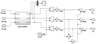
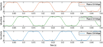
Figure 12 depicts the Simulink design of SVPWM power unit block. The control voltages generated by the power processing unit is shown in Figure 13.
Table 3. Electric vehicle parameters in this study
|
Parameter, Symbol |
Value (dimension) |
|
Vehicle mass, $M_{v}$ |
1500 kg |
|
Radius of wheel, $r_{d}$ |
0.28 m |
|
Frontal Area, $A_{f}$ |
2.26 m2 |
|
Coefficient of Rolling Resistance, $f_{r}$ |
0.01 |
|
Aerodynamic coefficient, $C_{d}$ |
0.28 |
|
Transmission Gear Ratio, $i_{g}$ |
3.29 |
|
Total Gear Ratio, $i_{o}$ |
0.95 |
|
Air Density, $\rho_{a}$ |
1.206 kg.m-3 |
|
Wheel Base, L |
2.7 m |
|
Distance between the gravity centre and the front wheel centre, $L_{a}$ |
1.134 m |
|
Height from Gravity Centre, $h_{g}$ |
0.6 m |
|
Transmission Efficiency, $\eta_{t}$ |
0.9 |
|
Acceleration due to Gravity, g |
9.8 m.s-2 |
Figure 11. Simulink model indirect vector controlled based PMSM fed electric vehicle
Figure 12. Simulink model of SVPWM PPU
Figure 13. Control voltages generated by SVPWM PPU
Operating the motor in accordance with the reference speed is fundamental for any electric vehicle. Performing simulation under both circumstances that is, steady speed varying torque and steady torque varying speed assess the validity of the specified system.
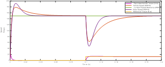
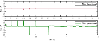
In the case of steady speed varying torque operation, the system is simulated for a time period of 0.2 s. For a constant speed command of 150 kmph, the initial value of command torque is held at zero, and then a step command torque of 12.9 Nm equal to the peak value is applied at time 0.1 s. The electromechanical torque generated by the PMSM motor varies in response to step input, as shown in Figure 14, and the motor speed curve drops at that point, rebounding to its command value in less than 0.04 s. The vehicle speed follows the motor speed in appropriate manner.
Figure 14. Torque and speed response for constant speed mode of operation
Figure 15. Torque and speed response for constant torque mode of operation
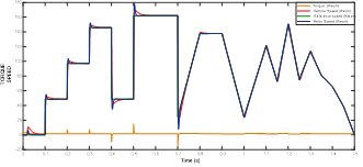
Figure 16. Zoomed response for staircase speed input from 0.1 s to 0.4 s
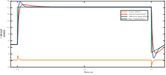
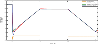
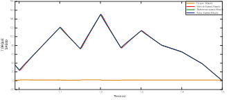
In the case of steady torque varying speed operation of the system, the drive curve is defined for a wide range of speeds for a time period of 1.5 s depicted in Figure 15. In this mode torque is kept constant to zero for entire period of simulation. The reference speed drive curve comprises of staircase speed signal from time 0.1 s to 0.4 s for duration of 0.3 s, step speed signal from time 0.5 s to 0.7 s for duration of 0.2 s, trapezoidal from time 0.7 s to 1s for a duration of 0.3 s and irregular surface from time 1s to 1.5 s for duration of 0.5 s. The zoomed figures of staircase, step, trapezoidal and irregular surface responses depicted in Figures 16-19 respectively. The motor speed is observed to follow the command speed with steady-state error zero and has a quicker time to settle at sudden changes in speed. This is observed especially in case of stair case and step speed inputs. The time to settle down is approximately less than 0.03 s. The FLC performs better in terms of fast response, low starting current, low overshoot, and low undershoot comparatively [27, 28].
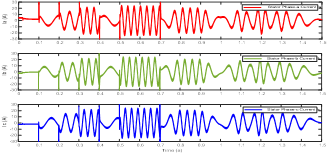
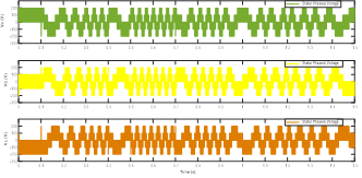
The PMSM drive dynamic response has been sighted under these conditions. Figure 20 depicts the d-axis and q-axis current waveforms. It can be spotted hat the q-axis current $i_{q s}$ oscillates first and then sets to table when it reaches the steady state condition, while d-axis current $i_{d s}$ is nearly zero for whole duration. This current peaking is observed only in the stair case and step command speed when there are sudden changes in speed signals. The three phase currents and voltages fed to stator of PMSM for entire simulation period of 1.5 s are shown in Figures 21 and 22 respectively. The findings suggest that the FLC can effectively manage rapid rise in command speed with minimal overshoot and undershoot as well as steady-state error. The recommended FLC was considered to have best performance in both transient and steady state conditions.
Figure 17. Zoomed response for step speed input from 0.5 s to 0.7 s
Figure 18. Zoomed response for trapezoidal speed input from 0.7 s to 1 s
Figure 19. Zoomed response for irregular speed input from 1 s to 1.5 s
Figure 20. d-axis and q-axis current waveforms of PMSM
Figure 21. Stator phase currents fed to PMSM stator from PPU
Figure 22. Phase voltages fed to PMSM stator from PPU
This paper gives us insight into the design of an electric vehicle with variable speed drive system. The results of Section 5 demonstrate that the effectiveness of an FLC based electric vehicle is good in terms of performance. The findings show that the responses were robust and the functionality of an electric vehicle is solid, consistent, stable, and unaffected by changes in parameters or operating conditions. Finally, it is concluded that the electric vehicle drive has potency and performance. In future research, the fuzzy logic concept can be extended in the controller design of predictive, adaptive, PID and neural network controllers utilized in electric vehicles. Further, this concept can apply to asynchronous and reluctance motors and speed responses are compared to the proposed electric vehicle model.
|
Mv |
vehicle mass, kg |
|
U |
vehicle speed, m.s-1 |
|
F |
tractive effort, N |
|
g |
gravitational acceleration, m.s-2 |
|
T |
torque, N.m |
|
V, v |
voltage, V |
|
i |
current, A |
|
f |
frequency, Hz |
|
p |
pole number |
|
Greek symbols |
|
|
δ |
mass factor |
|
$\alpha$ |
road surface elevation angle |
|
μ |
adhesion coefficient |
|
ρ |
air density, kgm-1 |
|
ղ |
efficiency |
|
Ψ |
flux linkages, wb |
|
ω |
angular speed, rad.s-1 |
|
θ |
electrical, mechanical angle, rad |
|
Subscripts |
|
|
a,b,c |
a,b,c phase windings |
|
d,q |
direct, quadrature phase windings |
|
s, r |
stator, rotor |
|
l |
leakage |
|
ref |
reference |
|
dc |
direct current |
|
tri |
triangular |
|
sw |
switching |
|
max, peak |
maximum |
|
mech |
mechanical |
|
Superscripts |
|
|
→ |
space vector |
|
a |
axis used as reference |
|
* |
reference |
[1] Bida, V.M., Samokhvalov, D.V., Al-Mahturi, F.S. (2018). PMSM vector control techniques-A survey. IEEE Conference of Russian Young Researchers in Electrical and Electronic Engineering, Moscow and St. Petersburg, Russia, pp. 577-581. https://doi.org/10.1109/EIConRus.2018.8317164
[2] Liu, T.T., Tan, Y., Wu, G., Wang, S.M. (2009). Simulation of PMSM vector control system based on Matlab/Simulink. International Conference on Measuring Technology and Mechatronics Automation, Zhangjiajie, China, pp. 343-346. https://doi.org/10.1109/ICMTMA.2009.117
[3] Guo, D., Dinavahi, V., Wu, Q., Wang, W. (2017). Sliding mode high speed control of PMSM for electric vehicle based on flux-weakening control strategy. 36th Chinese Control Conference (CCC), Dalian, China, pp. 3754-3758. https://doi.org/10.23919/ChiCC.2017.8027944
[4] Un-Noor, F., Padmanaban, S., Mihet-Popa, L., Mollah, M.N., Hossain, E. (2017). A comprehensive study of key electric vehicle (EV) components, technologies, challenges, impacts, and future direction of development. Energies, 10(8): 1217. https://doi.org/10.3390/en10081217
[5] Hadboul, R.M., Ali, A.M. (2021). Modeling, simulation and analysis of electric vehicle driven by induction motor. IOP Conference Series: Materials Science and Engineering, 1105(1): 012022. https://doi.org/10.1088/1757-899X/1105/1/012022
[6] Bouradi, S., Negadi, K., Araria, R., Marignetti, F. (2020). Z-source inverter for energy management and vector control for electric vehicle based PMSM. Journal Européen des Systèmes Automatisés, 53(6): 883-892. https://doi.org/10.18280/jesa.530614
[7] Abdellaoui, H., Ghedamsi, K., Mecharek, A. (2019). Performance and lifetime increase of the PEM fuel cell in hybrid electric vehicle application by using an NPC seven-level inverter. Journal Européen des Systèmes Automatisés, 52(3): 325-332. https://doi.org/10.18280/jesa.52031 4
[8] Türker, T., Buyukkeles, U., Bakan, A.F. (2016). A robust predictive current controller for PMSM drives. IEEE Transactions on Industrial Electronics, 63(6): 3906-3914. https://doi.org/10.1109/TIE.2016.2521338
[9] Sreejeth, M., Singh, M. (2018). Performance analysis of PMSM drive using hysteresis current controller and PWM current controller. IEEE International Students' Conference on Electrical, Electronics and Computer Science, Bhopal, India, pp. 1-5. https://doi.org/10.1109/SCEECS.2018.8546862
[10] Rathod, G., Thosar, A.G., Dhote, V.P., Zalke, R. (2018). PM synchronous motor drive for electric vehicles by using an adaptive controller. International Conference on Emerging Trends and Innovations in Engineering and Technological Research, Ernakulam, India, pp. 1-5. https://doi.org/10.1109/ICETIETR.2018.8529029
[11] Uysal, A., Gokay, S., Soylu, E., Soylu, T., Çaşka, S. (2019). Fuzzy proportional-integral speed control of switched reluctance motor with MATLAB/Simulink and programmable logic controller communication, Measurement and Control, 52(7-8): 1137-1144. https://doi.org/10.1177%2F0020294019858188
[12] Kaloko, B.S., Soebagio, M.H.P., Purnomo, M.H. (2011). Design and development of small electric vehicle using MATLAB/Simulink. International Journal of Computer Applications, 24(6): 19-23. https://doi.org/10.5120/2960-3940
[13] Janiaud, N., Vallet, F.X., Petit, M., Sandou, G. (2010). Electric vehicle powertrain simulation to optimize battery and vehicle performances. IEEE Vehicle Power and Propulsion Conference, Lille, France, pp. 1-5. https://doi.org/10.1109/VPPC.2010.5729141
[14] Chaibet, A., Larouci, C., Grunn, E. (2008). An electric simulator of a vehicle transmission chain coupled to a vehicle dynamic model. 34th Annual Conference of IEEE Industrial Electronics, Orlando, FL, USA, pp. 1578-1583. https://doi.org/10.1109/IECON.2008.4758189
[15] Ehsani, M., Gao, Y., Longo, S., Ebrahimi, K.M. (2018). Modern Electric, Hybrid Electric, and Fuel Cell Vehicles. CRC press.
[16] Larminie, J., Lowry, J. (2012). Electric Vehicle Technology Explained. John Wiley & Sons.
[17] Mohan, N. (2014). Advanced Electric Drives: Analysis, Control, and Modeling Using MATLAB/Simulink. John Wiley & Sons. https://doi.org/10.1002/9781118910962
[18] Ong, C.M. (1998). Dynamic simulation of electric machinery: Using MATLAB/SIMULINK Vol. 5: Upper Saddle River, NJ. Prentice Hall PTR.
[19] Srivastava, S., Chaudhari, M.A. (2020). Comparison of SVPWM and SPWM schemes for NPC multilevel inverter. IEEE International Students Conference on Electrical, Electronics and Computer Science, Bhopal, India, pp. 1-6. https://doi.org/10.1109/SCEECS48394.2020.131
[20] Li, B., Wang, C. (2016). Comparative analysis on PMSM control system based on SPWM and SVPWM. Chinese Control and Decision Conference, Yinchuan, China, pp. 5071-5075. https://doi.org/10.1109/CCDC.2016.7531902
[21] Chethan, G.N. (2019). Performance analysis of PMSM drive with Spacevector PWM and sinusoidal PWM fed VSI. International Conference on Power Electronics Applications and Technology in Present Energy Scenario, Mangalore, India, pp. 1-6. https://doi.org/10.1109/PETPES47060.2019.9003961
[22] Vujji, A., Dahiya, R. (2020). Design of PI controller for space vector modulation based direct flux and torque control of PMSM drive. First IEEE International Conference on Measurement, Instrumentation, Control and Automation Kurukshetra, India, pp. 1-6. https://doi.org/10.1109/ICMICA48462.2020.9242812
[23] Kar, B.N., Mohanty, K.B., Singh, M. (2011). Indirect vector control of induction motor using fuzzy logic controller. 10th International Conference on Environment and Electrical Engineering, Rome, Italy, pp. 1-4. https://doi.org/10.1109/EEEIC.2011.5874782
[24] Bose, B.K. (2002). Modern Power Electronics and AC Drives Vol. 123: Upper Saddle River, NJ. Prentice Hall.
[25] Sharma, K., Agrawal, A., Bandopadhaya, S., Roy, S. (2019). Fuzzy logic based multi motor speed control of electric vehicle. IEEE 5th International Conference for Convergence in Technology, Ernakulam, India, pp. 1-5. https://doi.org/10.1109/ICETIETR.2018.8529029
[26] Araria, R., Berkani, A., Negadi, K., Marignetti, F., Boudiaf, M. (2020). Performance analysis of DC-DC converter and DTC based fuzzy logic control for power management in electric vehicle application. Journal Européen des Systèmes Automatisés, 53(1): 1-9. https://doi.org/10.18280/jesa.530101
[27] Rajendran, A., Karthik, B. (2021). Design and analysis of fuzzy and PI controllers for switched reluctance motor drive. Materials Today, Proceedings, 37: 1608-1612. https://doi.org/10.1016/j.matpr.2020.07.166
[28] Mishra, T., Devanshu, A., Kumar, N., Kulkarni, A.R. (2016). Comparative analysis of hysteresis current control and SVPWM on fuzzy logic based vector controlled induction motor drive. IEEE 1st International Conference on Power Electronics, Intelligent Control and Energy Systems (ICPEICES), Delhi, India, pp. 1-6. https://doi.org/10.1109/ICPEICES.2016.7853632