Wisam Abdulabbas Abidalla* | Ahmed Sami Naser | Mohsin J. Nasir
© 2022 IIETA. This article is published by IIETA and is licensed under the CC BY 4.0 license (http://creativecommons.org/licenses/by/4.0/).
OPEN ACCESS
This research aims to find a suitable transportation rate formula for bed load. Laboratory experiments were conducted in a flume for monitoring and measuring the transportation of sediment particles (bed load) which move by jumping, rolling, or sliding within the flume. This study included two parts. The first part is experimenting using a flume and tracking the particles' movement by analysing the images taken by the camera. The measurements that have been taken are the amount of accumulated bed load particles at the end of the flume, which are distributed along a certain distance during a specific time, thus obtaining measuring data about the amount of accumulated bed load and values of moving distance and the required time for accumulating the particles at the flume end. The accumulated height of bed load is also measured. These experiments were conducted at different low-flow velocities. The second part includes the expression of a formula for bed load transportation rate, which is the product of multiplying the accumulated height of bed load by the velocity of bed load particles with distance at a certain time that was devised in the first part. Through the proposed method of obtaining the measurements in the first part Analysis of bed load particle velocity was done by using (π-theorem) from the results of experiments (Cv, V, ρ, ρS, µ, ds, L). To derive the formula of accumulated bed load height at flume end along a certain distance using Rayleigh’s method and using the results of the experiment (δ, V, g, ds). Finally, there can be found an expression of the bed load transportation rate formula. Checking was made for this formula, which was compared with other researchers' equations using statically measured. It was found that the derived formula was acceptable to calculate the transportation rate of bed load.
bed load, flume, formula, laboratory experimental, sediment transport rate
The transport rate of bed load is defined by some researchers, such as Einstein, as the transport of sediment particles in a thin layer just above the bed by sliding, rolling, and sometimes by jumping over a longitudinal distance [1]. Based on the triangle dune shape, van den Berg [2] defined this transport rate as follows: "the volumetric sediment transport rate involved with the celerity of bed forms per unite width and time, including the void, is equal to the product of dune cross-section area and dune celerity divided by the dune length". Shim and Duan [3] define transport rate in bed load as the amount of bed load particles transported along with flow on the bed surface over a period of time.
In general, bed load transport is defined as the amount of bed load particles that travel per a specific area per period by rolling, sliding, and salting. As for tracking bed load particles, many researchers have used cameras to track and analyse the velocity of bed load particles, such as Bracken et al. [4], which studies the motion of particles by tracking solid particles to find their velocity by using a high-speed camera. Furbish et al. [5] analysed the speed of sand particles and results from high-speed imaging of sand particles as they travel on a flat surface. Le Hir et al. [6] studied the velocity of sediment particles by measuring the velocity of particles using a commercial camera and predicting the probability density function of bed shear stress. Tsai et al. [7] studied the numerical model using measured average suspended sediment concentration and average flow velocity data to estimate velocity profiles and concentration profiles and calculate bed load transport rate. This numerical model will be used to evaluate the validity of a bed load formula when measurable load and average flow velocity are available. In this study, it was supposed that when the bed load moves by jumping, sliding, and salutation, they move to the end of the bed, the bed load accumulates and covers the distance of (L) at a certain time and with a thickness or height of (δ). Also, when the bed load particles move to the bed end, a front is formed that advances with time. Figure 1 shows a hypothetical plan where L is the distance that will be covered by the bed load during a certain period and can be called the moving distance, and a certain thickness can be called the thickness of the moving bed load (δ).
Through the moving distance and time, we can find the velocity, which can be called the velocity of the bed load. It is required to cover the moving distance (L), so the bed load transport rate can be calculated by multiplying the velocity of the bed load with the thickness of the moving bed load. The velocity of the bed load, time, and thickness will be measured and tracked along with the advanced front of the bed form by raster image analysis. This study was done in order to derive an equation to find a transportation rate formula by measuring the velocity of the advance of the bed load by analysing the images that were taken by the camera.
Figure 1. Hypothetical plan
As shown in Figure 2, sand with a grain size equal or less than 3 mm is used as a bed load in flumes with dimensions of 3 m length, 0.20 m width, and 0.30 m height.
Figure 2. Plan of the flume
Eight experiments were conducted at different flow velocities. A camera was used to record each experiment; the video was converted into a roster every five seconds. From the experiments, it was observed that when the particles of bed load move to the end of the flume, a front is made that progresses with time, so it should be tracking the moves of the bed form to get measurements for each experiment. Images of the moving bed load were analysed using AutoCAD raster design by measuring the distance of the bed load moving and recording the time from the above. Then it is possible to calculate the bed load velocity. The importance of finding the bed load velocity is to evaluate the discharge rate of bed load if you know the bed load thickness or height, so the height of bed load was also measured from image analysis, and the data measured are shown in Table 1.
Table 1. Values of measurements from experiments
|
Experimental No. |
Flo velocity (m/sec) |
Bed load velocity Cv(m/sec) |
Bed load height δ (m) |
Bed load transport rate measurements (m2/sec/unit width) |
|
1 |
0.045 |
0.0000573 |
0.04 |
1.900E-06 |
|
2 |
0.064 |
0.000400 |
0.022 |
8.300E-06 |
|
3 |
0.075 |
0.000580 |
0.015 |
8.500E-06 |
|
4 |
0.0801 |
0.00056 |
0.015 |
8.617E-06 |
|
5 |
0.102 |
0.00083 |
0.015 |
1.138E-05 |
|
6 |
0.1229 |
0.00099 |
0.015 |
1.148E-05 |
|
7 |
0.2083 |
0.0016 |
0.01 |
1.344E-05 |
|
8 |
0.223 |
0.002 |
0.007 |
1.364E-05 |
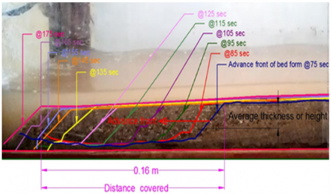
Figure 3 shows the image for experiment (no. 7). All eight experiments have been photographed and analysed, but in this study, the seventh experiment was randomly selected to clarify the terms of (L, δ, and Cv). The advance front at the first time (75 sec), the advance front at the final time (175 sec), and the distance between the two fronts (0.16 m). From the value of time difference between the two fronts and the value of moving distance, the bed load velocity can be measured at 0.0016 m/sec. The average bed load height was measured at 0.01 m. The bed load transport rate was also measured (1.344E-05 m2/sec/unite width).
(a)
(b)
(c)
Figure 3. (a) The image of the seventh experiment showing the resulting measurements (Advanced front, distance, and total time); (b) The image of the seventh experiment showing the resulting measurements - Initial time; (c) The image of the seventh experiment showing the resulting measurements - Second time
The aim of this study is to find the formula for the bed load velocity in terms of flow velocity, fluid properties, and sediment particle properties. In addition, the other objective is to estimate the expression for calculating the height of bed load in terms of gravity acceleration, grain size of sediment, and velocity of flow. Then the main aim is to derive a suitable bed load transportation formula.
3.1 The bed load velocity formula
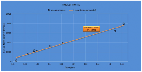
Initially, through the image analysis, the bed load velocity was measured. Also, when drawing it against the flow velocity, it was found to have a linear relationship between them as shown in Figure 4. That’s because Cv α V then Cv =K. Cv is the bed load velocity (m/sec), V is the flow velocity (m/sec), and K is the coefficient.
Figure 4. The relationship between flow velocity and bed load velocity
Experimental results (Cv, V, ρ, ρS, µ, g, ds, L) where Cv is the bed load velocity, V is the velocity of flow, ρ is the fluid density, ρs is the sediment density, µ is the kinetics viscosity coefficient, g is the acceleration of gravity, ds is the particle diameter, and L is the length of the bed, were used to predict the bed load coverage velocity [8]. Buckingham’s π-theorem is used to analyze. The dependent variable π1 is a function of the others πs are independent variables. Eqns. (1)-(5) were the dimensions of the groups derived from the Buckingham Theory method, which can be expressed as:
$\pi_{1}=\frac{C_{v}}{V}$ (1)
$\pi_{2}=\frac{\mu}{V L P}$ (2)
$\pi_{3}=\frac{L g}{V^{2}}$ (3)
$\pi_{4}=\frac{d_{s}}{L}$ (4)
$\pi_{5}=\frac{\rho_{s}}{\rho}$ (5)
Substituting the values π1, π2, π3, π4, and π5 in f (π1 π2, π3, π4, π5) =0 is gotten:
$F\left[C_{v} / V, \quad \mu / V L \rho, \quad L g / V^{2}, \quad d_{s} / L,\quad \rho_{s} / \rho\right]=0$ (6)
$C_{v} / V=\Phi\left[\mu / V L \rho, \quad L g / V^{2}, \quad d_{s} / L, \quad \rho_{S} / \rho\right]$ (7)
$C_{v} / V=\Phi\left[1 / R_{e}, \quad 1 / Fr^{2},\quad d_{s} / L, \quad \rho_{S} / \rho\right]$ (8)
Eqns. (6)-(8) is the process of developing an equation to determine the value of (Cv / V) in terms of Reynolds and Fraud's numbers, as well as the other variables in dimensionless groups. Where "Re" denotes the flow's Reynolds number and "Fr" denotes the flow's Fraud number.
Table 2 displays the experimental data obtained after dimensional analysis [9]. Linear regression by using SPSS [10] can be a prediction formula that explains the relationship between the ratio of the bed load coverage velocity (Cv) to the flow velocity (V) and other dimensionless groups [1/Re, 1/Fr2, ds / L, ρS / ρ].
The result of linear regression with R2 = 0.997 is shown in Eq. (9), which is driven by the application of the statistical programme SPSS. A linear relationship was found between the five dimensionless groups as:
$C v / V=(0.536 / R e)-\left(0.000001588 / F r^{2}\right)+\left(0.00279 \rho_{s} / \rho\right)$ (9)
So, the bed load coverage velocity (Cv) is:
$C v=\left\{(0.536 / R e)-\left(0.000001588 / F r^{2}\right)+\left(0.00279 \rho_{s} / \rho\right)\right\} V$ (10)
The Eq. (10) is similar to Eq. (11):
Cv =K V (11)
Then, from similarity the K is expressed as:
$K=(0.536 / R e)-\left(0.000001588 / F r^{2}\right)+\left(0.00279 \rho_{s} / \rho\right)$ (12)
Table 2. Experimental data resulting after dimensional analysis
|
Cv / V |
µ / V.L.ρ |
L.g / V2 |
ds / L |
ps / р |
|
0.001273333 |
0.013084967 |
8227.160494 |
0.001764706 |
2.65 |
|
0.00625 |
0.009200368 |
4067.382813 |
0.001764706 |
2.65 |
|
0.007733333 |
0.00785098 |
2961.777778 |
0.001764706 |
2.65 |
|
0.006991261 |
0.007351105 |
2596.629369 |
0.001764706 |
2.65 |
|
0.008137255 |
0.00577278 |
1601.30719 |
0.001764706 |
2.65 |
|
0.00805533 |
0.004791078 |
1102.989127 |
0.001764706 |
2.65 |
|
0.007681229 |
0.002826805 |
383.9692603 |
0.001764706 |
2.65 |
|
0.00896861 |
0.002640464 |
335.0157856 |
0.001764706 |
2.65 |
3.2 The bed load height formula
In order to calculate the bed load transport rate after the bed load velocity formula has been created in Eq. (11), an equation must be developed to calculate the height. Experimental results (δ, V, g, ds) were used to predict the thickness of the coverage layer of the bed load expression. Rayleigh’s method was used to analyse after the analysis was completed.
$\delta=\frac{d s . v^{b}}{(g . d s)^{b / 2}}$ (13)
where, b is a constant depending on the result of the regression. Nonlinear regression using SPSS can find the value of (b) with an R2 of 0.68. The resulting equation is:
$\delta=\frac{d s . v^{-1.963}}{(g . d s)^{-0.981}}$ (14)
Then, Eq. (15) is represented coverage thickness of the bed load expression.
$\delta=d s^{1.981} \cdot g^{0.981} \cdot V^{-1.963}$ (15)
3.3 The bed load transport rate formula
The bed load transport rate expressed as:
$q_{s}=\delta . C_{v}$ (16)
When substituting the Eq. (10) and Eq. (15) in the Eq. (16) result:
$q_{s}=K \cdot d s^{1.981} \cdot g^{0.981} \cdot V^{0.963}$ (17)
where, qs is the bed load transport rate per unite width (m2/sec) which is driven in this study.
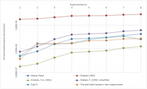
Firstly, the bed load transport rate was found according to the researchers' equations of Ettema and Mutel [11], Lajeuness et al. [12], Nielsen [13]. Secondly, the bed load transport rate was calculated according to Eq. (14). The results and measurement values of the bed load transport rate are shown in Table 3. From Figure 5, when graphically compared, it was seen that the bed load transport rate values calculated by Eq. (17) are closer to the measurement of the bed load transport rate.
Standard error (SE), root mean square error (RMSE), and standard bias (BIAS) [14] can be used to compare measured bed-load transport rate to that calculated by Einstein, H.A., Meyer-Peter, E., Nielsen, P., and Eq. (17).
SE= [Σ (qm-qc) 2 /N]0.5 (18)
RMSE=Σ [(qm-qc) / qm ]2 (19)
BIAS = Σ| (qm-qc) / qm | (20)
where, qm is the measured bed load transport rate, qc is the calculated bed load transport rate, and N is a data number.
The result of statistical measures that are shown in Table 4. In order to compare the equation obtained in this study (Eq. (17)) with other equations (Einstein, H.A., Meyer-Peter E., Nielsen, P., Nielsen, P. simplified), with applying statistical measures (SE, RMSE, BIAS), and these measures compare between the calculated bed load and the measured bed load. Statistically, the best equation is chosen when the values of SE, RMSE, and BIAS are the lowest.
Table 4 shows that the values obtained from applying the obtained equation are the lowest among all other equations. It was seen that the Eq. (17) has the smallest statistical measure values.
Figure 5. Graphically comparison between measurement bed load transport rate and that calculated by Einstein, H.A., Meyer-Peter, E., Nielsen, P., and Eq. (17)
Table 3. The bed load transport rate values for measurements and that calculated by Eq. (17)
|
Experimental |
qs measurement |
qs calculated by Eq. (17) |
Einstein, H.A. |
Meyer -Peter E. |
Nielsen, P. |
Nielsen,P. simplified |
|
1 |
1.900E-06 |
2.451E-06 |
9.172E-07 |
2.600E-06 |
8.976E-05 |
3.843E-06 |
|
2 |
8.300E-06 |
8.607E-06 |
1.198E-06 |
3.954E-06 |
9.518E-05 |
6.348E-06 |
|
3 |
8.500E-06 |
8.049E-06 |
2.161E-06 |
8.073E-06 |
1.092E-04 |
1.298E-05 |
|
4 |
8.617E-06 |
8.964E-06 |
3.560E-06 |
1.307E-05 |
1.238E-04 |
2.013E-05 |
|
5 |
1.138E-05 |
1.246E-05 |
3.898E-06 |
1.416E-05 |
1.268E-04 |
2.161E-05 |
|
6 |
1.148E-05 |
1.540E-05 |
4.256E-06 |
1.528E-05 |
1.298E-04 |
2.312E-05 |
|
7 |
1.344E-05 |
1.723E-05 |
5.460E-06 |
1.881E-05 |
1.391E-04 |
2.775E-05 |
|
8 |
1.364E-05 |
1.285E-05 |
6.372E-06 |
2.129E-05 |
1.453E-04 |
3.093E-05 |
Table 4. Comparison between measurement bed load transport rate and that calculated by Einstein, H.A., Meyer-Peter, E., Nielsen, P., and Eq. (17) using Statistical measures
|
Measures |
Eq. (17) |
Meyer - Peter |
Nielsen |
Einstein |
Nielson simplified model |
|
SE |
0.000003 |
0.000006 |
0.000157 |
0.000009 |
0.000015 |
|
RMSE |
0.298465 |
1.323186 |
2956.616317 |
3.364988 |
7.740637 |
|
BIAS |
1.196846 |
2.994850 |
121.376958 |
5.118856 |
7.366425 |
An equation is derived on the basis that the particles accumulate on the bed during the time. The particles move a long distance at any time at a thickness that is called the height of bed load. When comparing the calculated formula for bed load transport by Einstein, H.A., Meyer-Peter, E., Nielsen, P., and Eq. (17), it is seen that Eq. (17) has the smallest statistical measures, but cannot be compared with van den Berg [2] because the formula is suitable for high velocities of flow and the Eq. (17) is derived for low velocities. The Shim and Duan [3] formula cannot be compared to Eq. (17) because the estimating formula for sediment particle velocities without the thickness formula cannot estimate the bed load transport rate. Finally, the finding of the bed load rate is so important for channels, especially for small channels with low flow velocity, as it has been studied in the laboratory flume for this study. The resulting (derived) formulas can be used to find the bed load transport rate for unlined small channels with low flow velocity, which ranges from 0.045 to 0.233 m/sec. This formula is easy to use with clear parameters. The results show the important role of Reynolds and Fraud numbed in the determination of bed load transport rate. It was recommended that the same experiment be applied to the un-lining of channels with high water velocity.
[1] Wang, X., Zheng, J., Li, D., Qu, Z. (2008). Modification of the Einstein bed-load formula. Journal of Hydraulic Engineering, 134(9): 1363-1369.
[2] van den Berg, J.H. (1987). Bedform migration and bed-load transport in some rivers and tidal environments. Sedimentology, 34(4): 681-698. https://doi.org/10.1111/j.1365-3091.1987.tb00794.x
[3] Shim, J., Duan, J. (2019). Experimental and theoretical study of bed load particle velocity. Journal of Hydraulic Research, 57(1): 62-74. https://doi.org/10.1080/00221686.2018.1434837
[4] Bracken, L.J., Turnbull, L., Wainwright, J., Bogaart, P. (2015). Sediment connectivity: A framework for understanding sediment transfer at multiple scales. Earth Surface Processes and Landforms, 40(2): 177-188. https://doi.org/10.1002/esp.3635
[5] Furbish, D.J., Roseberry, J.C., Schmeeckle, M.W. (2012). A probabilistic description of the bed load sediment flux: 3. The particle velocity distribution and the diffusive flux. Journal of Geophysical Research: Earth Surface, 117(F3). https://doi.org/10.1029/2012JF002355
[6] Le Hir, P., Monbet, Y., Orvain, F. (2007). Sediment erodability in sediment transport modelling: can we account for biota effects? Continental Shelf Research, 27(8): 1116-1142. https://doi.org/10.1016/j.csr.2005.11.016
[7] Tsai, C.T., Tsai, C.H., Weng, C.H., Bair, J.J., Chen, C.N. (2010). Calculation of bed load based on the measured data of suspended load. Paddy and Water Environment, 8(4): 371-384. https://doi.org/10.1007/s10333-010-0216-4
[8] Haddadchi, A., Omid, M.H., Dehghani, A.A. (2013). Bedload equation analysis using bed load-material grain size. Journal of Hydrology and Hydromechanics, 61(3): 241. https://doi.org/0.2478/johh-2013-0031
[9] Mahoney, J.F., Yeralan, S. (2019). Dimensional analysis. Procedia Manufacturing, 38: 694-701.
[10] Li, L., Zhang, G., Zhang, J. (2019). Formula of bed-load transport based on the total threshold probability. Environmental Fluid Mechanics, 19(2): 569-581. https://doi.org/10.1007/s10652-018-9638-0
[11] Ettema, R., Mutel, C.F. (2004). Hans Albert Einstein: Innovation and compromise in formulating sediment transport by rivers. Journal of Hydraulic Engineering, 130(6): 477-487.
[12] Lajeunesse, E., Malverti, L., Charru, F. (2010). Bed load transport in turbulent flow at the grain scale: Experiments and modeling. Journal of Geophysical Research: Earth Surface, 115(F4). https://doi.org/10.1029/2009JF001628
[13] Nielsen, P. (1992). Coastal bottom boundary layers and sediment transport. World Scientific, 4: 340. https://doi.org/10.1142/1269
[14] Terlien, M.T. (1998). The determination of statistical and deterministic hydrological landslide-triggering thresholds. Environmental Geology, 35(2): 124-130. https://doi.org/10.1007/s002540050299