Prapada Watcharanat | Ponthep Vengsungnle | Paisarn Naphon*
© 2022 IIETA. This article is published by IIETA and is licensed under the CC BY 4.0 license (http://creativecommons.org/licenses/by/4.0/).
OPEN ACCESS
The risk of spreading the virus largely depends on the airflow behavior and the change in direction caused by the air supply and location of the exhaust air. The generated particles may travel long during sneezing, adversely affecting human bodies to defend against COVID-19 infectious diseases. This paper examines airflow path and airborne pollutant distribution in the nursing caring office room for COVID-19 patients ward at Princess Maha Chakri Sirindhorn Medical Center, Nakhornnayok province by computational fluid dynamics modeling and field measurement. Fifteen dummies of nursing staff stay in the room, and only one dummy (Patient) generated COVID-19. It is found that the generated particles during sneezing may travel a long distance as compared with the normal respiration and the ventilation system can effectively remove contaminants from the room and distribution in the room. From the obtained results, the keeping a social distancing should be more than 1.5 m for preventing the spread of the COVID-19 from person to person.
air ventilation, patient, office room, contaminant distribution
An infected person spreads COVID-19 (contaminant) by breathing, sneezing while not wearing a mask. The risk of spreading the virus depends on the airflow behavior, air supply direction, and the position of the exhaust air nozzle. Lipinski et al. [1] and Aganovic et al. [2] reviewed the current ventilation strategies used in the building to assess its modernization and describe in detail, especially for buildings with more dummies. For the hospital area, there are some works presented the air pollutants analysis. Effects of components inside the room, including panel and bed positions, temperature and supply airflow rate, and position on the exhaust air ventilation, were examined [3, 4]. Next, Ratajczak et al. [5] and Nejat et al. [6] experimentally investigated the visualization of airflows of smoke mixing. Kong et al. [7] evaluated the ventilation performance and assessed the exposure of healthcare workers by the patients in a confined experimental chamber. Sukarno et al. [8] improved the HVAC system using heat pipes for removing contaminants. Bivolarova et al. [9] studied the ventilated mattress performance of the exhaust ventilation system with an air fabric in a single-bed patient room with two heated dummies (Patients) and a doctor.
The operating room is an important area. A clean operating room is an essential guarantee in reducing infection rates during surgery. The energy consumption and comfort of the working room of three types of ventilation systems for operating rooms have been considered [10]. Next, Cho [11] examined airflow path and airborne pollutant distribution in a negative pressure isolation room by computational fluid dynamics modeling and field measurement. Swiercz [12] experimentally studied air quality in an office building by the mounted ventilation unit. Xue et al. [13] and Zhang et al. [14] considered the effect of the relevant parameters on the design of air ventilation systems in the operating room with different air change ratios. An air quality monitoring in the operating rooms has been conducted by Liang et al. [15], Lin et al. [16], and King et al. [17]. Cao et al. [18] considered the effect of airflow rate with air ventilation system on the surgical micro-environments. Fan et al. [19] evaluated the ventilation system performance in the operating room.
The objective of this study is to examine airflow path and airborne pollutant distribution in the nursing caring office room for COVID-19 patients ward at Princess Maha Chakri Sirindhorn Medical Center, Nakhornnayok province by computational fluid dynamics modeling and field measurement. Models from this study may be used to provide advice on the selection and design of suitable ventilation systems and the term appropriate social distance.
2.1 Governing equations
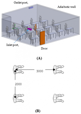
In a numerical model of the case study, airflow path and airborne pollutant distribution in the nursing caring office room for COVID-19 patients ward at Princess Maha Chakri Sirindhorn Medical Center are analyzed with a three-dimensional turbulent flow model by computational fluid dynamics modeling is shown in Figure 1, and Figure 3(A) with the assumptions are as following:
- Isothermal airflow indoor
- Excluded evaporation of particles
- Adiabatic boundary conditions
- Incompressible fluid
- Excluded gravitational force effect
- Constant air properties
The turbulent particles effect is excluded [20]. This is because of a low particle loading and comparatively small settling velocity. In addition, due to a low number of particles, the distribution of the particles is not altered by coagulation [21]. By viewing the computational domain as shown in Figure 1, a standard k-e turbulence model is used to simulate with the governing equations [21] as follows;
$\nabla \left( \rho U \right)=\,\,0$ (1)
$\frac{\partial \left( \rho U \right)}{\partial t}+\nabla \cdot \left( \rho UU \right)=\,\,\,-\nabla \left( P \right)+\nabla \cdot \left( {{\mu }_{eff}}\nabla U \right)+f$ (2)
$\frac{\partial \left( \rho \Phi \right)}{\partial t}+\nabla \cdot \left( \rho U\Phi \right)=\,\,\,\nabla \cdot \left( \frac{{{\mu }_{eff}}}{{{\sigma }_{\Phi }}}\nabla \Phi \right)+{{S}_{\Phi }}$ (3)
$\frac{\partial \left( \rho C \right)}{\partial t}+\nabla \cdot \left( \rho \left( U+{{U}_{S}} \right)C \right)=\nabla \cdot \left( \frac{{{\mu }_{eff}}}{{{\sigma }_{C}}}\nabla C \right)+{{S}_{C}}$ (4)
Standard k-e model [22].
$\frac{\partial \left( \rho k \right)}{\partial t}+div\left( \rho kU \right)=div\left[ \left( \frac{{{\mu }_{t}}}{{{\sigma }_{k}}}gradk \right) \right]+2{{\mu }_{t}}{{E}_{ij}}\cdot {{E}_{ij}}-\rho \varepsilon $ (5)
$\frac{\partial \left( \rho \varepsilon \right)}{\partial t}+div\left( \rho \varepsilon U \right)=div\left( \frac{{{\mu }_{t}}}{{{\sigma }_{\varepsilon }}}grad\varepsilon \right)+{{C}_{1\varepsilon }}\frac{\varepsilon }{k}2{{\mu }_{t}}{{E}_{ij}}\cdot {{E}_{ij}}-{{C}_{2\varepsilon }}\rho \frac{{{\varepsilon }^{2}}}{k}$ (6)
From the turbulence model [23], the constants are following:
$\begin{align} & {{\sigma }_{\varepsilon }}\,\,=\,\,1.3,\,\,\,\,\,\,\,{{\sigma }_{k}}\,\,=\,\,1.0 \\ & {{C}_{\varepsilon 2}}\,\,=\,\,1.92,\,\,{{C}_{\mu }}=0.09 \\ & {{C}_{\varepsilon 1}}\,\,=\,\,1.47 \\\end{align}$ (7)
2.2 Boundary equations
Initial conditions:
$U=\,\,{{U}_{in}},\,\,\,\,k\,\,=\,\,{{k}_{in}},\,\,\varepsilon \,\,=\,\,{{\varepsilon }_{in}},\,\,\,{{q}_{wall}}\,\,=\,\,0$ (8)
${{k}_{in}}\,\,=\,\,\frac{3}{2}{{\left( {{U}_{in}}I \right)}^{2}},\,\,{{\varepsilon }_{in}}\,\,=\,\,C_{\mu }^{3/4}\frac{{{k}^{3/2}}}{L}$ (9)
$I\,\,=\,\,\frac{{{U}^{'}}}{{{U}_{mean}}}\times 100\%\,$ (10)
In this study, the relative concentration from the mouth set as 1.0. U is the velocity of air, ρ is the density of air, P is pressure, Us is the settling particles velocity, C is the mass concentration of the particle. Φ is the scalar air quantity. σΦ is the turbulent diffusivity of Φ, σC is the turbulent diffusivity of C, which are 1.0. f is the body force due to the difference in air density [22]. SC is the generated particles rate, L is the characteristics length, and μeff is turbulent molecular viscosity sum [22]. For the zero equation turbulence model, wall functions are not needed for the region near the walls, where the algebraic equations of turbulent viscosity are applied directly [23].
Figure 1. The computation domain (A) and dummies distancing (B)
The fluid drag and the gravitational effects on the particle are equal. Therefore, a particle velocity with the same direction as gravitation and the drag coefficient [24] is obtained.
$\left| {{U}_{s}} \right|\,\,=\,\sqrt{\,\left[ \frac{4}{3}\frac{g{{d}_{p}}}{{{C}_{D}}}\frac{\left( {{\rho }_{p}}-{{\rho }_{a}} \right)}{{{\rho }_{a}}} \right]\,}$ (11)
${{C}_{D}}\,\,=\,\,\frac{24}{\operatorname{Re}}for\,\,\,\,\,\operatorname{Re}\langle 1$ (12)
${{C}_{D}}\,\,=\,\,\frac{24}{\operatorname{Re}}\left( 1+0.15{{\operatorname{Re}}^{2/3}} \right)\,\,\,\,for\,\,\,\,\,1\langle \operatorname{Re}\langle 1000$ (13)
where, Re is the relative Reynolds number based on the particle and air velocities.
The complex geometry [25], the N-point supply opening model, describes all variables at the supply inlet. For outlet boundary conditions, the supply airflow in and out the boundaries are specified the same values. The turbulent viscosity function is applied directly [26] for the boundary zone and is set as zero normal gradients $\left(\frac{\partial C}{\partial n}=0\right)$. Due to a little the deposited particle in the airflow direction, the deposited particle is an insignificant effect on the main flow [27].
2.3 Numerical procedure
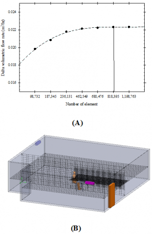
A commercial software ANSYS Fluent package, a three-dimensional standard k-e turbulent flow model is applied to solve the model. Based on the SIMPLEC algorithm [28], the coupling with velocity and pressure is employed in the numerical process with the main assumptions as mentioned above for considering two models with different dummies, as shown in Figure 2. Based on the actual number of human stay inside the nursing caring office room, 15 number of dummies are analyzed with initial conditions are set the constant supply airflow rate as 600 m3/hr, 900 m3/hr, and 1200 m3/hr. The residual criteria convergence is set as 10-6 for the ended numerical process. The computer with a dual CPUs socket 2011 V.3, 16 cores-32 threads, 32 GB memory, and 2133 MHz frequency is used for the procedure calculation.
Figure 2. The models used in the present analysis for model A and model B
2.4 Grid independent tests
The grid configuration for the present analysis is shown in Figure 3. The numerical procedure is performed with three different grid numbers (6.80*105, 8.10*105, and 11.98*105) to obtain the accuracy of the predicted results. Due to a discrepancy of volume flow rate less than 1% (810,000 and 1,198,000), the 819,000 is obtained for a satisfactory solution.
Figure 3. Grid independent test and grid configuration
3.1 Predicted results verification
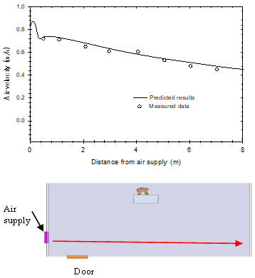
One ventilation system is constructed at the rear for the suction head and front left for the supply head of the nursing caring office room for the COVID-19 patient ward to eliminate the risk and optimize ventilation measurement hung on the wall. It is induced from the outside and forced into the room, as shown in Figure 2. In this study, the inlet air velocity at different positions is measured by airflow measurement (FESTO) with an accuracy of 0.01% of full scale. The measuring points of the temperature and the experiment air velocity are shown in Figure 4(b). For the measuring method, it is assumed that working people stay in the room only one. The variation of air temperature velocity at different positions of the office room is shown in Figure 4. The inlet air temperature is kept constant (30℃) and supply airflow rates of 600 m3/hr, 900 m3/hr, and 1200 m3/hr. The velocity distributions are measured in front of the supply port line, as shown in Figure 4(a). The predicted results are compared with the present measured data from the present study. It can be found that the predicted airflow velocity between the predicted results and the measured data is in reasonable agreement and gives average errors of 4.58%.
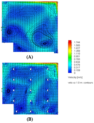
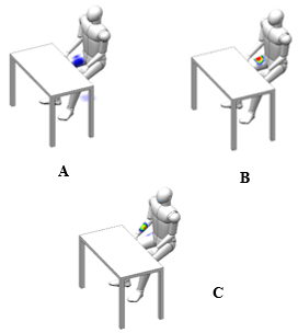
The air velocity contours at various positions for model A and model B are shown in Figure 5. The predicted results show that the velocity from the supply head regions of the two models spread throughout the nursing caring office room. The model is performed in case ventilation systems for the only one dummy staying in the room (model A) and fifteen for model B, as shown in Figure 2. However, for model B, fifteen dummies stay in the room. In model B, more dummy stay in the room than in model A, which will block the airflow in the room. Therefore, the airflow in model B has more circulation flow points than in the first, as shown in Figure 5. In addition, the airflow pattern for different dummies is shown in Figure 6. It is found that the airflow circulation occurs at the between zone dummy. A swirling flow can carry germs from one person to another for the closed distancing if sneezing occurs, as shown in Figure 6 (C). However, for long distancing between dummy, it prevents the transmission of the COVID-19 disease from human to human, as shown in Figure 6 (B).
Figure 4. Comparison of the predicted air velocity with the measured air velocity
Figure 5. Velocity contour of air inside the office room for the top view of model A and model B
Figure 6. Velocity contour of airflow inside the office room for the font view for different dummies
A streamline of air to visualize the airflow field within the nursing caring office room of model A for different airflow rates are shown in Figure 7. It can be seen clearly that a flow field of air from the supply head region spreads throughout the nursing caring office room and finally directs toward the suction head at the rear zone, which the centrifugal fans installed. It is indicated that the nursing caring office room coupled with the ventilation systems effectively affects air movement from one location to another.
Figure 7. Stream lines air flow for (A) 600 m3/hr, (B) 900 m3/hr, and (C) 1200 m3/hr
Table 1. The relevant parameter for the numerical analysis
|
Parameters |
values |
|
Saliva diameter (Particle), µm [29] |
90 |
|
Outlet saliva (Particle) velocity from the mouth, m/s [29] |
14.3 |
|
Number of saliva (Particle) |
30 |
|
Saliva density, kg/m3[21] |
600 |
|
Analysis temperature, ℃ |
30 |
|
Saliva flow rate, L/s [30] |
4.75 |
|
Cross section area of mouth, cm2[30] |
9.11 |
3.2 Cased study for the sneezing
For the case study of the coughing, there are some work presented the numerical analysis of the influence of generating ways of the droplets or particles on the transport and distribution of the droplets or particles indoors [21]. However, the problem and the boundary condition used in the numerical analysis are different. Outlet velocity from the mouth for the sneezing process is set at 14.3 m/s [29], and the saliva density of 600 kg/m3. The outlet velocity of normal respiration process is periodic and that of coughing or sneezing process is pulse [21]. The assumed velocity as boundary conditions in simulation is depicted in Figure 8. For this study, for simplification in the simulation, we assume sneezing once from the patient who stays in the room's middle zone (A long transport distance, high concentration). Table 1 presents the relevant parameters and other boundary conditions used in the present study. The study [21] shows that the particle with a large diameter only transports within 0.5-1.0 m, and the large generated particles are less than 5% of all the particles. Therefore, the generated fine particles with a size of 90 µm are considered. This means that the density of the particle has no significant effect on the flow phenomena.
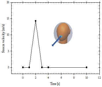
Figure 8. Outlet velocity of the particles from the sneezing
In the present study, flow behaviors have been predicted in the respiratory periods (6 s). The sneezing process begins at the 2 s periods at the middle zone of the nursing caring office room. Unlike the normal respiration process, the sneezing process may produce a large number of particles of droplets. Relatively more minor airflow volume for the normal breathing process, the transport distance of particles or droplets generated by normal respiration of patients is limited. Therefore, the flow patterns of air in the inhaling and exhaling processes are not considered in the present study.
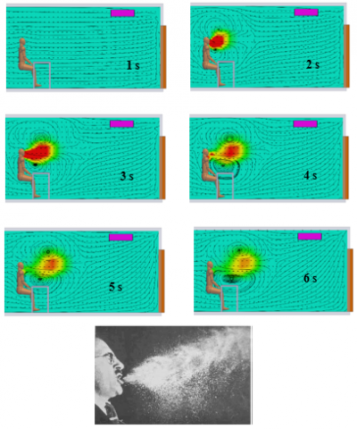
Figure 9 gives the mass fraction of water and airflow pattern at different times with the sneezing process. It is seen that the air and particle spread more widely in the front direction from the human. The maximum mass fraction of water and the maximum velocity occurs at the 2nd-3rd second after sneezing and reduce within 1.5 m away from the human. Due to higher momentum, the sneezing process causes a long transport distance of air and particles compared to the normal respiration process. Figure 9 also compares the predicted airflow pattern with the measured data [21]. It can be found that the flow pattern seems reasonable. Figure 9 also shows that the generated particles during the sneezing process travel a long distance, adversely affecting human bodies to defend against COVID-19 infectious diseases. From the obtained results, the keeping a social distancing should be more than 1.5 m for preventing the COVID-19 disease from person to person.
Figure 9. Mass fraction of water and flow pattern of the particles from the sneezing process from the present study and compared with experimental results [21]
Figure 10. Positions of the precipitated particles for (A) 600 m3/hr, (B) 900 m3/hr, and (C) 1200 m3/hr
Figure 11. Number of precipitated particles at different time for (A) 600 m3/hr, (B) 900 m3/hr, and (C) 1200 m3/hr
Figures 10, 11 show the position and number of particle concentrations settling on the ground several times. It is found that the particle precipitate rate is significantly different for the different supply airflow rates. For a 600 m3/hr volume air flowrate, most of the particles precipitate on the inner zone of the right thigh at 3.6-4.1 seconds. At 3.7-3.8 seconds, the maximum particles precipitate rate occurs. For a higher volume airflow rate at 900 m3/hr, most particles precipitate faster and precipitate on the middle zone of the right thigh zone and then the right arm zone for 1200 m3/hr. However, it depends on the position and the face direction for sneezing, including the air ventilation system.
The risk of spreading the virus largely depends on the airflow behavior and the change in direction caused by the air supply and location of the exhaust air. This paper examines airflow path and airborne pollutant distribution in the nursing caring office room for COVID-19 patients ward at Princess Maha Chakri Sirindhorn Medical Center, Nakhornnayok province by computational fluid dynamics modeling and field measurement. It is found that the traveling distance and spreading of the generated particles for the sneezing process is higher than that for normal respiration. From the obtained results, we recommend keeping a social distancing more than 1.5 m. Good personal habits, the person should be covering the nose and mouth when sneezing. However, there are many assumptions excluding the relevant parameters in the present study. Therefore, the results should only be used as the cautions. The following work may be analyzed the relevant parameter effects on the complex airflow phenomena including dummy activities inside the room for zoning airflow management for preventing infectious COVID-19 diseases.
This work received funds from the Faculty of Engineering. The authors would like to thank the Faculty of Engineering, Srinakharinwirot University (SWU), for their financial support in this research.
[1] Lipinski, T., Ahmad, D., Serey, N., Jouhara, H. (2020). Review of ventilation strategies to reduce the risk of disease transmission in high occupancy buildings. International Journal of Thermofluids, 7(8): 100045. https://doi.org/10.1016/j.ijft.2020.100045
[2] Aganovic, A., Cao, G., Fecer, T., Ljungqvist, B., Lytsy, B., Radtke, A., Reinmuller, B., Traversari, R. (2021). Ventilation design conditions associated with airborne bacteria levels within the wound area during surgical procedures: A systematic review. Journal of Hospital Infection, 113: 85-95. https://doi.org/10.1016/j.jhin.2021.04.022
[3] Jung, C.C., Wu, P.C., Tseng, C.H., Su, H.J. (2015). Indoor air quality varies with ventilation types and working areas in hospitals. Building and Environment, 85: 190-195. https://doi.org/10.1016/j.buildenv.2014.11.026
[4] Choi, N., Yamanaka, T., Sagara, K., Momoi, Y., Suzuki, T. (2019). Displacement ventilation with radiant panel for hospital wards: Measurement and prediction of the temperature and contaminant concentration profiles. Building and Environment, 160: 106197. https://doi.org/10.1016/j.buildenv.2019.106197
[5] Ratajczak, K., Amanowicz, L., Szczechowiak, E. (2020). Assessment of the air streams mixing in wall-type heat recovery units for ventilation of existing and refurbishing buildings toward low energy buildings. Energy & Buildings, 227: 110427. https://doi.org/10.1016/j.enbuild.2020.110427
[6] Nejat, P., Ferwati, M.S., Calautit, J., Ghahramani, A. Sheikhshahrokhdehkordi, M. (2021). Passive cooling and natural ventilation by the windcatcher (Badgir): An experimental and simulation study of indoor air quality. thermal comfort and passive cooling power, Journal of Building Engineering, 41: 102436. https://doi.org/10.1016/j.jobe.2021.102436
[7] Kong, X., Guo, C., Lin, Z., Duan, S., He, J., Ren, Y., Ren, J. (2021). Experimental study on the control effect of different ventilation systems on fine particles in a simulated hospital ward. Sustainable Cities and Society, 73: 103102. https://doi.org/10.1016/j.scs.2021.103102
[8] Sukarno, R., Putra, N., Hakim, I.I., Rachman, F.F., Mahli, T.M.I. (2021). Utilizing heat pipe heat exchanger to reduce the energy consumption of airborne infection isolation hospital room HVAC system. Journal of Building Engineering, 35(4): 102116. https://doi.org/10.1016/j.jobe.2020.102116
[9] Bivolarova, M.P., Melikov, A.K., Mizutani, C., Kajiwara, K., Bolashikov, Z.D. (2016). Bed-integrated local exhaust ventilation system combined with local air cleaning for improved IAQ in hospital patient rooms. Building and Environment, 100: 10-18. https://doi.org/10.1016/j.buildenv.2016.02.006
[10] Alsved, M., Civilis, A., Ekolind, P., Tammelin, A., Andersson, A.E., Jakobsson, J., Svensson, T., Ramstorp, M., Sadrizadeh, S., Larsson, P.A., Bohgard, M., Temkiv, T.S., Londahl, J. (2018). Temperature-controlled airflow ventilation in operating rooms compared with laminar airflow and turbulent mixed airflow. Journal of Hospital Infection, 98(2): 181-190. https://doi.org/10.1016/j.jhin.2017.10.013
[11] Cho, J. (2019). Investigation on the contaminant distribution with improved ventilation system in hospital isolation rooms: Effect of supply and exhaust air diffuser configurations. Applied Thermal Engineering, 148: 208-218. https://doi.org/10.1016/j.applthermaleng.2018.11.023
[12] Świercz, E.Z. (2020). Improvement of indoor air quality by way of using decentralized ventilation. Journal of Building Engineering, 32: 101663. https://doi.org/10.1016/j.jobe.2020.101663
[13] Xue, K., Cao, G., Liu, M., Zhang, Y., Pedersen, C., Mathisen, H.M., Stenstad, L.I., Skogås, J.G. (2020). Experimental study on the effect of exhaust airflows on the surgical environment in an operating room with mixing ventilation. Journal of Building Engineering, 32: 101837. https://doi.org/10.1016/j.jobe.2020.101837
[14] Zhang, Y., Cao, G., Feng, G., Xue, K., Pedersen, C., Mathisen, H.M., Stenstad, L.I., Skogås, J.G. (2020). The impact of air change rate on the air quality of surgical microenvironment in an operating room with mixing ventilation. Journal of Building Engineering, 32: 101770. https://doi.org/10.1016/j.jobe.2020.101770
[15] Liang, C.C., Wu, F.J., Chien, T.Y., Lee, S.T., Chen, C.T., Wang, C., Wan, G.H. (2020). Effect of ventilation rate on the optimal air quality of trauma and colorectal operating rooms. Building and Environment, 169: 106548. https://doi.org/10.1016/j.buildenv.2019.106548
[16] Lin, T., Zargar, O.A., Lin, K.Y., Juina, O., Sabusap, D.L., Hu, S.C., Leggett, G. (2020). An experimental study of the flow characteristics and velocity fields in an operating room with laminar airflow ventilation. Journal of Building Engineering, 29: 101184. https://doi.org/10.1016/j.jobe.2020.101184
[17] King, K.G., Delclos, G.L., Brown, E.L., Emery, S.T., Yamal, J.M., Emery, R.J. (2021). An assessment of outpatient clinic room ventilation systems and possible relationship to disease transmission. American Journal of Infection Control, 49: 808-812. https://doi.org/10.1016/j.ajic.2021.01.011
[18] Cao, G., Kvammen, I., Hatten, T.A.S., Zhang, Y., Stenstad, L.I., Kiss, G., Skogås, J.G. (2021). Experimental measurements of surgical microenvironments in two operating rooms with laminar airflow and mixing ventilation systems. Energy and Built Environment, 2: 149-156. https://doi.org/10.1016/j.enbenv.2020.08.003
[19] Fan, M., Cao, G., Pedersen, C., Lu, S., Stenstad, L.I., Skogas, J.G. (2021). Suitability evaluation on laminar airflow and mixing airflow distribution Strategies in operating rooms: A case study at St. Olavs Hospital. Building and Environment, 194(1): 107677. https://doi.org/10.1016/j.buildenv.2021.107677
[20] Elghobashi, S. (1994). On predicting particle-laden turbulent flows. Applied Scientific Research, 52: 309-329. https://doi.org/10.1007/BF00936835
[21] Zhao, B., Zhang, Z., Li, X. (2005). Numerical study of the transport of droplets or particles generated by respiratory system indoors. Building and Environment, 40: 1032. https://doi.org/10.1016/J.BUILDENV.2004.09.018
[22] Versteeg, H.K., Malalasekera, W. (1995). Computational Fluid Dynamics. Longman Group.
[23] Launder, B.E., Spalding, D.B. (1973). Mathematical Models of Turbulence, Academic Press.
[24] Hinds, W.C. (1982). Aerosol Technology: Properties, Behavior, and Measurement of Airborne Particles. New York, Wiley.
[25] Zhao, B., Li, X., Yan, Q. (2003). A simplified system for indoor airflow simulation. Building and Environment, 38(4): 543-552. https://doi.org/10.1016/S0360-1323(02)00182-8
[26] Chen, Q., Xu, W. (1998). A zero-equation turbulence model for indoor air flow simulation. Energy and Buildings, 28: 137-144. https://doi.org/10.1016/S0378-7788(98)00020-6
[27] Nazaroff, W.W., Cass, G.R. (1989). Mathematical modelling of indoor aerosol dynamics. Environmental Science and Technology, 23: 157-165. https://doi.org/10.1021/es00179a003
[28] Van Doormal, J.P., Raithby, G.D. (1984). Enhancements of the SIMPLEC method for predicting incompressible fluid flows. Numerical Heat Transfer, 7: 147-163. https://doi.org/10.1080/01495728408961817
[29] Pendar, P.R., Pascoa, J.C. (2020). Numerical modeling of the distribution of virus carrying saliva droplets during sneeze and cough. Physics of Fluids, 32: 083305. https://doi.org/10.1063/5.0018432
[30] Beni, H.M., Hassani, K., Khorramymehr, S. (2019). In silico investigation of sneezing in a full real human upper airway using computational fluid dynamics method. Computer Methods and Programs in Biomedicine, 177: 203-209. https://doi.org/10.1016/J.CMPB.2019.05.031