Maria Mahabub | M. Ferdows | M. Gluam Murtaza | Giulio Lorenzini* | E.E. Tzirtzilakis
© 2022 IIETA. This article is published by IIETA and is licensed under the CC BY 4.0 license (http://creativecommons.org/licenses/by/4.0/).
OPEN ACCESS
This paper focuses on the theoretical and numerical investigation of the unsteady, viscous, incompressible, two-dimensional laminar boundary layer flow of a Newtonian biomagnetic fluid over a stretching sheet under the influence of an applied magnetic field in the presence of heat transfer. The magnetic field is induced by a magnetic dipole placed below the stretching sheet. The magnetic field intensity represents the magneto-thermo-mechanical coupling. This allows exclusion of the biofluid that is distant from the sheet at Curie temperature to avoid further magnetization. The unsteadiness of the flow is discernible in the fluid flow properties. The mathematical model of the problem conforms to the principles of Magnetohydrodynamics (MHD) and Ferrohydrodynamics (FHD). In this work, the study is performed on a specific biofluid, human blood. The modified Stokes principle is used to implement the model under the assumption that along with the three thermodynamic variables P, ρ, and T, the Biomagnetic Fluid Dynamics (BFD) fluid behavior can be characterized as a function of magnetization M. To describe the physical problem, a coupled non-linear system of ordinary differential equations subject to appropriate boundary conditions is derived from Navier-Stokes and thermal energy equations by performing non-dimensionalization of the considered variables. To solve these equations, the dsolve routine in the MAPLE software is used. Numerical results for flow profiles and the local skin friction coefficient (Cfx) and the local Nusselt number (Nux) are discussed for different values of unsteadiness parameter (A), biomagnetic interaction parameter (B) and a rational quantity (ϵ). The achieved results are compared with previously published work for steady state flow, and they seem to be in good agreement. It is found that MHD and FHD interaction parameters affect significantly on the velocity, temperature and pressure field. A successful completion will bring interesting results for better understanding of the biomagnetic fluid flow characteristics and can be beneficial to medical and bioengineering applications; particularly for estimating the characteristics of blood flow in stenosed arteries.
boundary layer flow, biomagnetic fluid, magneto-thermo-mechanical, unsteady flow, stretching sheet, magnetic field
Unsteady fluid flow hinges upon time dependent flow properties—velocity, pressure, temperature etc. This type of fluid flow can be observed in human body due to much impulsive body movement, vibration, unintentional abrupt body acceleration while riding any vehicle or in various kinds of physical competition. In addition, this type of flow might occur in a cardiovascular disease—the leading cause of death.
In 2015, the World Health Organization (WHO) reported approximately 17.7 million deaths due to cardiovascular diseases, consisting of 31% of all global deaths. Approximately 7.4 million of these deceased population suffered from coronary heart disease and 6.7 million suffered from stroke. A “myocardial infarction” or a heart attack happens when the blood flow to some portion of the heart muscle is blocked by a formed clot in an artery. Due to inadequate blood flow and consequently less oxygen and nutrients, the portion of the heart muscle gets damaged. The intensity of the damage depends on a variety of factors: the size and the location of the clot and the duration of the block. Longer duration causes extensive damage to the muscle. There are other kinds of diseases which are concerned with narrowing of blood vessels such as peripheral artery disease, vascular diseases, atherosclerosis etc. In these diseases the irregular blood flow might fall prey to unsteadiness in the flow. Peripheral artery disease (PAD) is a well-known circulatory problem where narrowed arteries lessen the blood flow to limbs. As known, arteries carry oxygen and nutrients through blood from the heart to every part of the body such as the brain, kidneys, intestines, arms, legs, and heart itself. When PAD is developed, extremities such as legs do not get sufficient blood flow to match the demand of the body. Two other types of diseases that are caused by disruptive blood flow are vascular disease and atherosclerosis. Vascular disease is an abnormal condition of the blood vessels that occurs where turbulent blood flow takes place, e.g., when the direction of blood flow in the arteries changes abruptly. Atherosclerosis, on the other hand, is the narrowing of the vessels that carry blood to the heart. Atherosclerosis occurs due to fat deposit built up in the artery walls. Hereby the inevitable usefulness of the study of blood flow in a narrow blood vessel. A substantial amount of work has been carried out on biological fluids. Among them the most important and characteristic one is blood. Also, some extensive amounts of works have been done using the effects of magnetic field and heat transfer. Needless to say, all these studies bear immense potential for biomedical engineering applications and clinical medicine.
Kafoussias and Tzirtzilakis provided mathematical analyses that dealt with the flow and heat transfer of a BFD fluid in a channel with stretching sheet [1]. Tzitzilakis et al. [2] studied turbulent flow of a BFD fluid in a rectangular channel under the influence of an applied magnetic field. Andersson and Valnes [3] investigated the heated ferrofluid flow over a stretching sheet. They performed their study in the presence of a magnetic dipole. Under certain conditions, BFD fluid, human blood has been observed to exhibit viscoelastic behavior [4-6]. Misra and Shit [7] presented mathematical models to investigate the biomagnetic viscoelastic fluid flow over a stretching sheet and in a channel with stretching walls. They fluid was considered to flow under the action of a magnetic field that is externally produced by a magnetic dipole. In another work, Misra and Shit [8] studied the heated Ferro-fluid flow over a linear stretching sheet under the influence of an applied magnetic field. Further Misra et al. [9] mathematically analyzed the steady incompressible second grade electrically conducting fluid flow in a channel perfused by a uniform transverse magnetic field. There are several mathematical studies on the blood flow such as arterial blood flow in the presence of body exercise by Mwapinga [10], blood flow through a narrow, catheterized artery by Kumar et al. [11], arterial blood flow during electromagnetic hyperthermia by Misra et al. [12], MHD effects on stenosed blood flow by Haik et al. [13], and so on. The mathematical analyses of BFD fluid flow have been known to serve several important biomedical application-based research such as study on various types of magnetically controlled drug carrier systems by Ruuge and Rusetski [14], approaches for drug delivery to particular destinations within the human body by Voltairas et al. [15], and so on. Researchers have performed comparative numerical studies of biomagnetic fluid flow over the years. Tzirtzilakis and Kafoussias [16] have presented comparative study of a BFD fluid flow over a stretching sheet under the action of an applied magnetic field and mathematical models for biomagnetic fluid flow and applications [17]. Some other research works on comparative numerical studies are mathematical modeling of BFD that is suitable for describing the Newtonian blood flow controlled by an applied magnetic field by Tzirtzilakis [18], mathematical models of the blood flow in a stenosed channel under the influence of a steady localized magnetic field by Tzirtzilakis [19], numerical analysis for BFD problems applying stream function vorticity by Tzirtzilakis [20], the study of biomagnetic fluid flow under the impact of a steady magnetic field in an aneurysmal geometry by Tzirtzilakis [21], numerical analysis of BFD fluid flow over a stretching sheet in the presence of heat transfer by Tzirtzilakis and Tanoudis [22], BFD fluid flow under the impact of an applied magnetic field in a curved square duct by Papadopoulos and Tzirtzilakis [23], BFD fluid flow under the action of a uniform localized magnetic field in a channel by Tzirtzilakis and Loukopoulos [24], mathematical model of biomagnetic fluid Tzirtzilakis [18]. A substantial amount of works has been done on BFD fluid flow on a stretching sheet with unsteady velocity such as numerical analysis of unsteady stagnation point flow over a stretching or shrinking sheet with prescribed heat flux [25-27].
In this paper, the biofluid is studied under two considerations: there is a stretching sheet with unsteady velocity and the stretching sheet is under the influence of a magnetic dipole. The observed variables/properties of the fluid flow are velocity, pressure and temperature. These properties depend on dimensionless unsteadiness parameter A and biomagnetic parameter B.
An unsteady laminar flow of an incompressible, viscous, and electrically conducting BFD fluid and with heat transfer is assumed to be confined in half space (y > 0) above a sheet. This sheet is characterized as impermeable, flat, elastic,
$\vec{\nabla }.\vec{q}\,\,=\,\,0$ (1)
$\frac{\partial \text{u}}{\partial \text{t}}+\vec{q}.\vec{\nabla }u\,\,=\frac{\partial {{U}_{\infty }}}{\partial t}-\frac{1}{\rho }\frac{\partial p}{\partial x}+\frac{1}{\rho }{{\mu }_{0}}M\frac{\partial H}{\partial x}+\nu {{\nabla }^{2}}u$ (2)
$\frac{\partial v}{\partial t}+\vec{q}.\vec{\nabla }v\,\,=\,\,-\frac{1}{\rho }\frac{\partial p}{\partial y}+\frac{1}{\rho }{{\mu }_{0}}M\frac{\partial H}{\partial y}+\nu {{\nabla }^{2}}v$ (3)
$\rho \mathrm{C}_{\mathrm{p}} \frac{\partial \mathrm{T}}{\partial \mathrm{t}}+\rho \mathrm{C}_{\mathrm{p}} \overrightarrow{\mathrm{q}} \cdot \vec{\nabla} \mathrm{T}^{+} \mu_{0} \mathrm{~T} \frac{\partial \mathrm{M}}{\partial \mathrm{T}} \overrightarrow{\mathrm{q}} \cdot(\vec{\nabla} \mathrm{H})=\mathrm{K} \nabla^{2} \mathrm{~T}+\mu \varphi$ (4)
with boundary conditions:
$\mathrm{y}=0: \mathrm{u}=\mathrm{U}_{\mathrm{w}}, \mathrm{v}=0, \mathrm{~T}=\mathrm{T}_{\mathrm{w}}$
$\mathrm{y} \rightarrow \infty: \mathrm{u} \rightarrow \mathrm{U}_{\infty}, \mathrm{T} \rightarrow \mathrm{T}_{\mathrm{c}}, \mathrm{p}+1 / 2 \rho \mathrm{q}^{2}=$ constant (5)
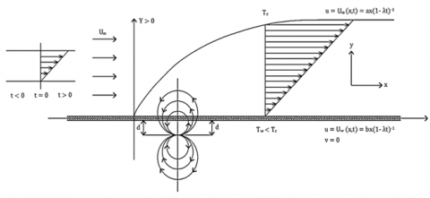
and stretched with a velocity Uw (x,t). The velocity of the fluid becomes U∞ (x,t), as moved far away from this sheet. Below this sheet, at a distance d, there is a magnetic dipole engendering a magnetic field that is strong enough to have the biomagnetic fluid saturated. As far as the temperature is concerned, a fixed temperature Tw is maintained for the sheet. At a further distance from the sheet, the fluid retains the Curie Temperature Tc, higher than the wall temperature in magnitude. Unsteady fluid flow, i.e. time dependent flow as it implies by definition, in this study the properties like velocity and pressure of biomagnetic fluid flow are considered as time dependent functions. An overview of the flow model and co-ordinate system of biomagnetic fluid flow is depicted in Figure 1.
Following the mathematical models, presented by Tzirtzilakis and Tanoudis [22] and Suali et al. [25], under the above-mentioned assumptions, the governing continuity, momentum and heat conservation equations can be written as:
$\left\{ 2\left[ {{\left( \frac{\partial u}{\partial x} \right)}^{2}}+{{\left( \frac{\partial v}{\partial y} \right)}^{2}}+{{\left( \frac{\partial v}{\partial x}+\frac{\partial u}{\partial y} \right)}^{2}} \right] \right\}$ (6)
In the equations above, the free stream velocity is $U_{\infty}$ $=\mathrm{ax} /(1-\lambda \mathrm{t})$; sheet stretching velocity is $\mathrm{U}_{\mathrm{w}}=\mathrm{bx} /(1-\lambda \mathrm{t})[25]$; $\mathrm{u}$ is the velocity component of the fluid in the $\mathrm{x}$ direction and $\mathrm{v}$ is the velocity component of the fluid in the y direction, and $\vec{q}=(\mathrm{u}, \mathrm{v}) ; v$ is the kinetic viscosity which is the ratio of dynamic viscosity $\mu$ and density $\rho$.
Moreover, ∇2 is the Laplacian operator in two-dimension whereas φ is the dissipation function given by Tzirtzilakis and Tanoudis [22]:
Here the terms ${{\mu }_{0}}M\frac{\partial H}{\partial x}$ and ${{\mu }_{0}}M\frac{\partial H}{\partial y}$ in (2) and (3), depict the components of the magnetic force per unit volume along x and y directions respectively. They are dependent on the presence of the magnetic gradient caused by the magnetic dipole. These gradients are absent when the magnetic forces disappear. On the left-hand side of the thermal energy Eq. (4), the third term accounts for heating due to adiabatic magnetization. As cited by Andersson and Valnes [3], the components Hx, Hy of the magnetic field $\,\vec{H}(x,y)=({{H}_{x}},{{H}_{y}})$, are given by the following expressions:
${{H}_{x}}(x,y)=-\frac{\partial V}{\partial x}=\frac{\gamma }{2\pi }\frac{{{x}^{2}}-{{\left( y+d \right)}^{2}}}{{{\left[ {{x}^{2}}+{{\left( y+d \right)}^{2}} \right]}^{2}}}$ (7)
${{H}_{y}}(x,y)=-\frac{\partial V}{\partial y}=\frac{\gamma }{2\pi }\frac{2x\left( y+d \right)}{{{\left[ {{x}^{2}}+{{\left( y+d \right)}^{2}} \right]}^{2}}}$ (8)
$V(x,y)=\frac{\alpha }{2\pi }\frac{x}{{{x}^{2}}+{{\left( y+d \right)}^{2}}}$ (9)
In the above equations d is the distance of the magnetic dipole situated below the sheet, α is the dimensionless distance, defined as a = ${{\left( \frac{a}{\nu (1-\lambda t)} \right)}^{1/2}}$d, V refers to the scalar potential of the magnetic dipole [3 and, in it γ = α.
As such, the magnitude $\left\| {\vec{H}} \right\|=H$ is given by:
$H(x,y)={{\left[ H_{x}^{2}+H_{y}^{2} \right]}^{1/2}}=\frac{\gamma }{2\pi }\frac{1}{{{x}^{2}}+{{\left( y+d \right)}^{2}}}$ (10)
and the magnetic field gradients are given by:
$\frac{\partial H}{\partial x}$=$-\frac{\gamma }{2\pi }$$\frac{2x}{{{(y+d)}^{4}}}$ (11)
$\frac{\partial H}{\partial y}$=$\frac{\gamma }{2\pi }\left[ -\frac{2}{{{\left( y+d \right)}^{3}}}+\frac{4{{x}^{2}}}{{{\left( y+d \right)}^{5}}} \right]$ (12)
Since it has been assumed that $\overrightarrow{\mathrm{H}}(\mathrm{x}, \mathrm{y})$ has enough strength for saturating the biomagnetic field, the magnetization M is usually established by the fluid temperature and the magnetic field intensity. Considerably, the variation of magnetization with respect to temperature T can be expressed and estimated by M = K (Tc − T), an approximation given by ANDERSSON and VALNES [3]. Here K is a constant, namely the pyro-magnetic co-efficient and Tc is the Curie temperature. The biofluid becomes no longer magnetized, as soon as it reaches the Curie temperature. The reason behind this is the increasing intensity H of the magnetic field. However, following the consideration by Matsuki et al. [28], it is experimentally proven that
$\mathrm{M}=\mathrm{KH}\left(\mathrm{T}_{\mathrm{c}}-\mathrm{T}\right)$ (13)
To have no further magnetization, in this study, Eq. (13) restricts to ignore the biofluid at a further distance from the sheet, at Curie temperature Tc.
Figure 1. Geometry of unsteady fluid flowa
In this part, the following non-dimensional variables given by Tzirtzilakis and Tanoudis [22] and Suali et al. [25] are introduced:
$\xi(\mathrm{x})=\left(\frac{\mathrm{a}}{v(1-\lambda \mathrm{t})}\right)^{1 / 2} \mathrm{x}$ (14)
$\eta(\mathrm{y})=\left(\frac{\mathrm{a}}{v(1-\lambda \mathrm{t})}\right)^{1 / 2} \mathrm{y}$ (15)
$\psi(\xi, \eta)=v \xi f(\eta)$ (16)
$\theta(\xi, \eta)=\frac{\mathrm{T}_{\mathrm{c}}-\mathrm{T}}{\mathrm{T}_{\mathrm{c}}-\mathrm{T}_{\mathrm{w}}}=\theta_{1}(\eta)+\xi^{2} \theta_{2}(\eta)$ (17)
$\mathrm{P}(\xi, \eta)=\frac{\mathrm{p}}{\mathrm{a} \mu}(1-\lambda t)=-\mathrm{P}_{1}(\eta)-\xi^{2} \mathrm{P}_{2}(\eta)$ (18)
where, $\xi(\mathrm{x}), \eta(\mathrm{y}), \psi(\xi, \eta), \mathrm{P}(\xi, \eta), \theta(\xi, \eta)$ are dimensionless co-ordinates in $\mathrm{x}$ and $\mathrm{y}$, stream function, pressure, and temperature, respectively.
Substituting Eqns. (11)-(18) into the Eqns. (2)-(4) and then equating the coefficients of equal powers of ξ, up to $\xi^{4}$, an approach to the transformation is performed in the following manner:
The velocity components are calculated as follows:
$\mathrm{u}=\frac{\partial \psi}{\partial \mathrm{y}}=\left(\frac{\mathrm{a}}{1-\lambda \mathrm{t}}\right) \mathrm{xf}^{\prime}(\eta)$ (19)
$\mathrm{v}=-\frac{\partial \psi}{\partial \mathrm{x}}=-\left(\frac{\mathrm{a} v}{(1-\lambda \mathrm{t})}\right)^{1 / 2} \mathrm{f}$ (20)
The boundary value problem (BVP) given by Eqns. (1) ̴ (5) then reduces to the following system of coupled nonlinear partial differential equations:
$\mathrm{f}^{\prime \prime \prime}+\mathrm{ff}^{\prime \prime}-\left(\mathrm{f}^{\prime}\right)^{2}+2 \mathrm{P}_{2} \frac{2 \alpha^{2} \mathrm{~B} \theta_{1}}{(\eta+\alpha)^{6}}+\mathrm{A}\left(1-\frac{1}{2} \mathrm{f}^{\prime}-\frac{1}{2} \eta \mathrm{f}^{\prime \prime}\right)$$=0$ (21)
$\mathrm{P}_{1}^{\prime}-\mathrm{f}^{\prime \prime}-\mathrm{f} \mathrm{f}^{\prime}-\frac{2 \alpha^{2} \mathrm{~B} \theta_{1}}{(\eta+\alpha)^{5}}+\frac{\mathrm{A}}{2} \eta=0$ (22)
$\mathrm{P}_{2}^{\prime}-\frac{2 \alpha^{2} \mathrm{~B} \theta_{2}}{(\eta+\alpha)^{5}}+\frac{6 \alpha^{2} \mathrm{~B} \theta_{1}}{(\eta+\alpha)^{7}}=0$ (23)
$\theta_{1}^{\prime \prime}+\operatorname{Pr} \mathrm{f} \theta_{1}^{\prime}-\mathrm{A} \operatorname{Pr} \theta_{1}^{\prime} \frac{\eta}{2}+2 \theta_{2}+\alpha^{2} \mathrm{~B} \operatorname{PrEc}$
$\left\{\frac{2 \mathrm{f} \theta_{2}}{(\eta+\alpha)^{5}}-\left(\theta_{1}-\mathrm{T}_{\varepsilon}\right)\left[\frac{2 \mathrm{f}^{\prime}}{(\eta+\alpha)^{6}}+\frac{6 \mathrm{f}}{(\eta+\alpha)^{7}}\right]\right\}+\operatorname{EcPr}\left(\mathrm{f}^{\prime \prime}\right)^{2}$$=0$ (24)
$\theta_{2}^{\prime \prime}-\operatorname{Pr}\left(2 \theta_{2} f^{\prime}-f \theta_{2}^{\prime}\right)+\alpha^{2} B E c \operatorname{Pr}$
$\left\{\left(\theta_{1}-\mathrm{T}_{\varepsilon}\right)\left[\frac{2 \mathrm{f}^{\prime}}{(\eta+\alpha)^{8}}+\frac{4 \mathrm{f}}{(\eta+\alpha)^{9}}\right]-\theta_{2}\left[\frac{2 \mathrm{f}^{\prime}}{(\eta+\alpha)^{6}}+\frac{6 \mathrm{f}}{(\eta+\alpha)^{7}}\right]\right\}$$-\operatorname{Pr} \mathrm{A}\left[\theta_{2}+\frac{\eta}{2} \theta_{2}^{\prime}\right]=0$ (25)
The transformed boundary conditions assure the form:
$\eta=0: \mathrm{f}=0, \mathrm{f}^{\prime}=\frac{\mathrm{b}}{\mathrm{a}}=\epsilon, \theta_{1}=1, \theta_{2}=0$
$\eta \longrightarrow \infty: \mathrm{f}^{\prime} \longrightarrow 1, \theta_{1} \longrightarrow 0, \theta 2 \longrightarrow 0, \mathrm{P}_{1} \longrightarrow-\mathrm{P}_{\infty}, \mathrm{P}_{2} \longrightarrow 0$ (26)
The physical dimensionless parameters that have appeared in the Eqns. (21)-(26) are:
$\Pr =\frac{\mu {{C}_{p}}}{K}$ (Prandtl number)
${{T}_{\varepsilon }}$ =$\frac{{{T}_{c}}}{({{T}_{c}}-{{T}_{w}})}$ (Dimensionless temperature)
B =$\frac{\gamma }{2\pi }$$\frac{{{\mu }_{0}}KH(0,0)\left( {{T}_{c}}-{{T}_{w}} \right)\,\rho }{{{\mu }^{2}}}$ (Biomagnetic interaction parameter)
Ec =$\frac{{{U}_{\infty }}^{2}}{{{C}_{p}}\left( {{T}_{c}}-{{T}_{w}} \right)}$ (Eckert number)
$\alpha=\left(\frac{a}{v(1-\lambda t)}\right)^{1 / 2} d$ (Dimensionless distance)
$\epsilon=\frac{b}{a}$ (Ratio of stretching parameter and the free stream velocity parameter)
$A= \frac{\lambda }{a}$ (Unsteadiness parameter)
The system of Eqns. (21)-(25), subjected to the boundary condition (26), is a seven-parameter non-linear coupled system. It describes the unsteady flow of a biomagnetic fluid over a stretching sheet under the effect of magnetization.
Numerical calculations have been performed for different values of dimensionless parameters for the considered problem. The solutions are obtained by using MAPLE software [29]. The Maple differential equation solver (dsolve) has been used to solve the problem. Both step size Δη, and the convergence criteria are set to the default values: 0.01 and 10−6, respectively. Until convergence is achieved, an automatic adjustment of the missing initial derivative is performed by the algorithm incorporated in the software. The procedure has been well established by its accuracy and robustness in numerous publications [30-34]. The asymptotic boundary conditions ηmax are substituted by a finite value of 0.6. It ensures that all numerical solutions precisely follow the far field asymptotic values. The far field boundary conditions in (26) are replaced by a finite value of 0.6 for similarity variable ηmax. Thus, when ηmax=0.6, f'(0.6)=0 and P(0.6)=θ(0.6)=0. The command dsolve successfully substitutes the BVP by an initial value problem (IVP).
In relevant to this study, for biomagnetic fluid, blood, the density ρ = 1050 kg m-3, viscosity μ = 3.2x10⁻³ kg m-1s-1, and the maximum velocity U∞ = 3.048 x10⁻² m s-1 [20, 21]. The magnetic dipole is positioned under the stretching sheet at a distance d = 10-4 m. The Curie temperature for blood is considered as Tc = 41℃ and the temperature of blood is considered as Tw = 37℃ (Tzirtzilakis [21]). Using Tc and Tw, the dimensionless temperature Tε is calculated to be 78.5. For these temperatures, the measurements for blood are adopted as specific heat under constant pressure Cp = 3.9x10³ J Kg-1K-1, thermal conductivity K = 0.5 J m-1s-1K-1 by Chato [35]. Although μ, Cp, K of any fluid including blood depends on temperature, the Prandtl number Pr can be a constant. The Prandtl number Pr for the above-mentioned values is calculated to be 25. Furthermore, for these values Eckert number is derived as Ec = 5.96x10⁻⁸. Near the magnetic field β0 = 4 − 8T, the saturated magnetization value M0 is 40 A m-1 Tzirtzilakis [21]. For these values, and for β0 = 4T, M0 = 40A m-1, d =10-4; the calculated value for B is 164. If the strength of the magnetic field at the wall is 8T, the B becomes 336. Note that, the value B = 0 corresponds to hydrodynamic flow. The dimensionless distance α is taken to be equal to 1 by Sajid et al. [36]. The values of unsteadiness parameter A and the ratio ϵ are assumed by “trial and error” method. Here, the most crucial quantities of physical interest are the local skin friction coefficient $C_{f_{x}}$ and local rate of heat transfer coefficient Nux, also known as local Nusselt number. These quantities are defined by Misra and Shit [8]:
$\mathrm{C}_{\mathrm{f}}=-\frac{\tau_{\mathrm{w}}}{\rho \mathrm{U}_{\infty}^{2} / 2}$ (27)
$\mathrm{Nu}_{\mathrm{x}}=\left.\frac{\mathrm{x}}{\left(\mathrm{T}_{\mathrm{c}}-\mathrm{T}_{\mathrm{w}}\right)} \frac{\partial \mathrm{T}}{\partial \mathrm{y}}\right|_{\mathrm{y}=0}$ (28)
where, τw is the wall shear stress defined as:
$\tau_{\mathrm{w}}=\left.\mu \frac{\partial \mathrm{u}}{\partial \mathrm{y}}\right|_{\mathrm{y}=0}$ (29)
Using Eqns. (14), (15), (17), (19) and (20), the above-mentioned quantities can be obtained as:
$\mathrm{C}_{\mathrm{f}_{\mathrm{x}}}=-2 \mathrm{f}^{\prime \prime}(0) \operatorname{Re}_{\mathrm{x}}^{-1 / 2}$ (30)
$\mathrm{Nu}_{\mathrm{x}}=-\left[\theta_{1}^{\prime}(0)+\xi^{2} \theta_{2}^{\prime}(0)\right] \operatorname{Re}_{\mathrm{x}}^{1 / 2}$ (31)
where, $\mathrm{Re}_{\mathrm{x}}$ is the local Reynolds number $\mathrm{Re}_{\mathrm{x}}=\frac{\mathrm{U}_{\infty} \mathrm{x}}{v}$ [23], -f"(0) is the dimensionless wall shear parameter and $\theta^{\prime}(0)=\left[\theta_{1}^{\prime}(0)+\xi^{2} \theta_{2}^{\prime}(0)\right]$ is the dimensionless wall heat transfer parameter. The flow field is seemingly influenced by the values of the biomagnetic interaction parameter $B$. When $B=$ 0 (hydrodynamic case), at infinity $\mathrm{P}_{2}$ becomes zero (constant). So, it is more suitable to consider replacing the dimensionless wall heat transfer parameter $-\theta^{\prime}(0)=-\left[\theta_{1}^{\prime}(0)+\xi^{2} \theta_{2}^{\prime}(0)\right]$ by $\theta^{*}(0)=\frac{\theta_{1}^{\prime}(0)}{\left.\theta_{1}^{\prime}(0)\right|_{\mathrm{B}=0}}$, namely the coefficient of the heat transfer rate at the sheet [25]. Also, $\mathrm{P}_{2}(0)$ can be defined as the dimensionless wall pressure parameter.
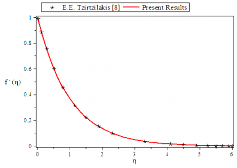
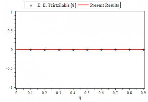
The numerical results of the present study together with comparison to studies in the open literature are presented in this section. The transformed Eqns. (21) to (25) with boundary condition (26) are numerically solved with the help of an efficient Runge – Kutta - Fehlberg 4th order numerical method using Maple 14. During the solution process, different values of the parameters A, B and ϵ are used. The range of parameter values used for numerical computations are: 0 ≤ A ≤ 3, 0 ≤ B ≤ 328 and 0.5 ≤ ϵ ≤ 2.2. Figures 2, 3 represents the result of a comparison between the Maple and finite difference precision numerical solutions for a steady state case with B = 0, A = 0, ϵ = 1, Pr = 7, Ec = 0, α = 1, Tε=2 by setting ηmax = 6 and 0.9. The velocity and pressure profiles for the steady and hydrodynamic case with B = 0 are in excellent agreement with those obtained by Tzirtzilakis [8].
Figure 2. Comparison of dimensionless velocity f ¢(η)
Figure 3. Comparison of dimensionless pressure P2 (η)
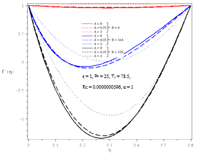
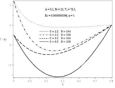
Figures 4,5 illustrates the velocity profiles $f^{\prime}(\eta)$ for various $B, A$ and $\epsilon$. Both are plotted against $\eta$. Figure 4 reveals the effects of $A$ and $B$ on the velocity profile and it can be inferred that under the influence of a stronger magnetic field, the fluid velocity decreases. In addition, the opposite results occur for increasing unsteadiness parameter for the case $B=0,164$ and 328. Note that for $\mathrm{B}=164$, the velocity increases near the wall and decreases far from the wall which cross one point occurring at a value of $\eta=0.3$. When these velocity profiles are observed, it is noticed from Figure 4 that for $B=164$ and $\mathrm{A}=0.35$, velocity starting from a boundary value $\mathrm{f}^{\prime}(0)=1$ tends to decrease to $f^{\prime}(0.22)=-0.106384$ and then increase to the boundary value $f^{\prime}(0.6)=1$. Similarly for $B=164$ and $\mathrm{A}=3$, this lowest velocity is: $\mathrm{f}^{\prime}(0.29)=0.0137628$; for $\mathrm{B}=$ 328 and $\mathrm{A}=0.35, \mathrm{f}^{\prime}(0.28)=-1.30197$; for $\mathrm{B}=328$ and $\mathrm{A}=3, \mathrm{f}^{\prime}(0.3)=-0.94128$. These velocity profiles happen to be depicted as parabolic trajectories. In case of the steady case $(A=0)$, it is noticed in Figure 4 that at some point the dimensionless velocity coincides with the unsteady one $(\mathrm{A} \neq 0)$ for biomagnetic parameter $\mathrm{B}=164$ (biomagnetic field strength 4T). For instance: when A $=0.35$ (unsteady) f $'(\eta)$ coincides with the steady profile at approximately $(0.154$, $-0.0319)$ and for $\mathrm{A}=3$ at $(0.296,0.0152)$. Boundary layer thickness is therefore higher with $B=328$. Figure 5 shows that the velocity profile increases with increasing values of $\epsilon$ from the surface to the fluid further away from the surface in two sets of numerical solutions. For $B=164$, starting from $f^{\prime}(0)=$ $0.5$, velocity decreases to $f^{\prime}(0.21)=-0.480572$ and from $f^{\prime}(0)$ $=2.2$, it decreases to $f^{\prime}(0.3)=0.887956$; then increases to the boundary value $f^{\prime}(0.6)=1$. Similarly for $B=328$, these decreased velocities are: for $B=328, f^{\prime}(0.27)=-1.599639$ and $f^{\prime}(0.24)=-0.28782$ starting from $f^{\prime}(0)=0.5$ and $2.2$ respectively.
Figure 4. Variation of dimensionless velocity f ¢(η) for different B and A
Figure 5. Variation of dimensionless velocity f ¢(η) for different ϵ and A
Figures 4,5 illustrates the velocity profiles $f^{\prime}(\eta)$ for various $B, A$ and $\epsilon$. Both are plotted against $\eta$. Figure 4 reveals the effects of $A$ and $B$ on the velocity profile and it can be inferred that under the influence of a stronger magnetic field, the fluid velocity decreases. In addition, the opposite results occur for increasing unsteadiness parameter for the case $\mathrm{B}=0,164$ and 328. Note that for $\mathrm{B}=164$, the velocity increases near the wall and decreases far from the wall which cross one point occurring at a value of $\eta=0.3$. When these velocity profiles are observed, it is noticed from Figure 4 that for $B=164$ and $A=0.35$, velocity starting from a boundary value $f^{\prime}(0)=1$ tends to decrease to $f^{\prime}(0.22)=-0.106384$ and then increase to the boundary value $f^{\prime}(0.6)=1 .$ Similarly for $B=164$ and $\mathrm{A}=3$, this lowest velocity is: $\mathrm{f}^{\prime}(0.29)=0.0137628 ;$ for $\mathrm{B}=$ 328 and $\mathrm{A}=0.35, \mathrm{f}^{\prime}(0.28)=-1.30197 ;$ for $\mathrm{B}=328$ and $A=3, f^{\prime}(0.3)=-0.94128$. These velocity profiles happen to be depicted as parabolic trajectories. In case of the steady case $(A=0)$, it is noticed in Figure 4 that at some point the dimensionless velocity coincides with the unsteady one $(A \neq$ 0) for biomagnetic parameter $\mathrm{B}=164$ (biomagnetic field strength 4T). For instance: when A $=0.35$ (unsteady) f' $(\eta)$ coincides with the steady profile at approximately $(0.154,-$ $0.0319)$ and for $\mathrm{A}=3$ at $(0.296,0.0152)$. Boundary layer thickness is therefore higher with $\mathrm{B}=328$. Figure 5 shows that the velocity profile increases with increasing values of $\in$ from the surface to the fluid further away from the surface in two sets of numerical solutions. For $B=164$, starting from $f^{\prime}(0)=$ $0.5$, velocity decreases to $f^{\prime}(0.21)=-0.480572$ and from $f^{\prime}(0)$ $=2.2$, it decreases to $f^{\prime}(0.3)=0.887956$; then increases to the boundary value $\mathrm{f}^{\prime}(0.6)=1$. Similarly for $\mathrm{B}=328$, these decreased velocities are: for $B=328, f^{\prime}(0.27)=-1.599639$ and $f^{\prime}(0.24)=-0.28782$ starting from $f^{\prime}(0)=0.5$ and $2.2$ respectively.
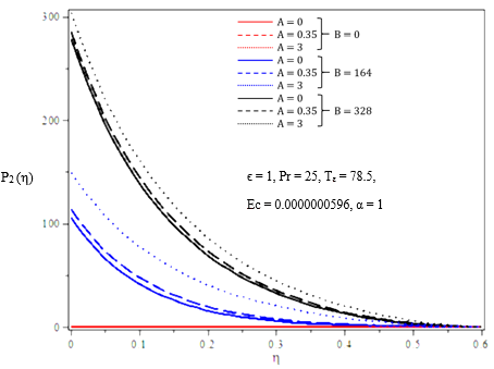
Figure 6. Variation of dimensionless pressure P2 (η) for different B and A
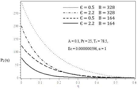
Figure 7. Variation of dimensionless pressure P2 (η) for different ϵ and B
Figures 6 and 7 depict the effects of unsteadiness parameter A and ϵ with the change of biomagnetic parameter B on the dimensionless pressure P2 (η). For hydrodynamic (B = 0) case (Figure 5) the flow coincides with the origin describing that B has no significant effect on pressure. With increase in B, dimensionless pressure increases. Also Figure 6, implicates that this increment in greater for larger values of unsteadiness parameter A. From Figure 7, it is evident that as ϵ increases, P2 (η) decreases. As the pattern of any of the graphs in Figures 6 and 7 is looked at, it is easily come to sight that pressure decreases gradually from a highest value and as η increases, it approaches to the boundary asymptotically.
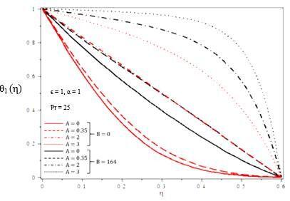
In Figures 8 and 9 temperature profiles are plotted against η in the form of dimensionless temperature θ1 (η) for various values of biomagnetic parameter B, unsteadiness parameter A and ϵ. As to the observation, when the biomagnetic interaction parameter B decreases, the dimensionless temperature θ1 (η) decreases. Recall that, B is the strength of the magnetic field generated by the magnetic dipole that is placed under the stretching sheet. Also, from Figure 8 it is evident that with increasing unsteadiness parameter A, the temperature becomes increased. As the pattern of the graphs of the dimensionless temperature is concerned, it is observed that for the hydrodynamic state (B = 0) when A < 2 and ϵ ≥ 1 the temperature drops from a highest value and approaches the boundary in an asymptotic manner. An interesting phenomenon is observed when B = 0, A= 2 and when B = 164, A = 0.35. In both the cases the dimensionless temperature θ1 (η) decreases almost linearly. From Figure 9 it is evident that, temperature is decrescent from the higher temperature region near the wall to the region away from the wall for increasing values of ϵ.
Figure 8. Variation of dimensionless temperature θ1 (η) for different B and A
Figure 9. Variation of dimensionless temperature θ1 (η) for different ϵ and B
Figure 10. Variation of the wall shear parameter − f'' (0)
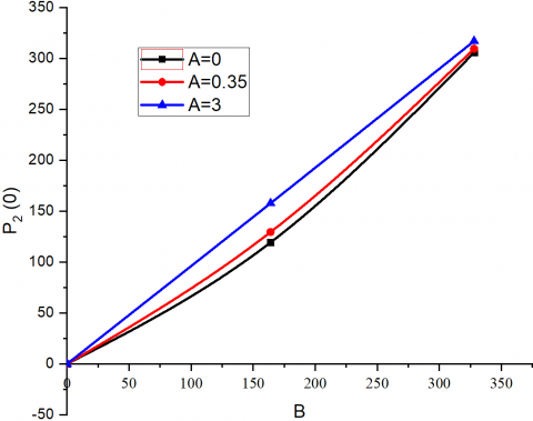
Figure 11. Variation of wall pressure parameter P2 (0)
Figure 12. Variation of the wall heat transfer parameter θ*(0)
Figures 10-12 graphically represents the results of the similarity solutions for the wall heat transfer. The results are shown for A as a function of biomagnetic parameter B. From Figure 10, as B increases in the blood, the wall shear increases asymptotically. The effect of A on the dimensionless wall shear is also investigated. It is found that wall shear decreases with the parameter A. Figure 11 shows that as the parameter B increases, the wall pressure increases. This effect can also be seen on the wall pressure as A increases. For A = 2, 3 wall shear parameter and wall pressure parameter increases almost linearly with respect to B, whereas for A = 0, 0.1, 0.35 wall shear parameter shows nonlinear increment with B. From Figure 12, we can see that for A = 0 and 0.1, θ*(0) vary almost linearly with respect to the increase of B. As we increase the value of A other than the above θ*(0) represents nonlinear profile. This is due to the transport of blood from higher temperature near the wall to the lower temperature far away from the wall.
In this paper, a numerical study has been carried out for the two-dimensional problem of the flow of a BFD fluid over a stretching sheet with heat transfer and magnetization. A similarity transformation has been employed for the reduction of the partial differential equations into nonlinear coupled ordinary differential equations. The effects of the dimensionless parameters A, ϵ and B on the fluid flow have been discussed here and the numerical results obtained here have been compared with the previously published results. All data have been acquired by using a dsolve routine in MAPLE software. However, significant results that have been found in this study are summarized as follows:
The change in velocity $f^{\prime}(\eta)$ with the change in unsteadiness parameter A is dependent upon the biomagnetic interaction parameter B. Velocity decreases with increasing B and increases with increasing A. But for B = 164 this phenomena get reversed.
Pressure P2 (η) increases with increasing B and this increment is greater for increasing A. On the other hand, P2 (η) decreases with increasing ϵ.
Temperature θ1 (η) increases with the increment of B and A, whereas it decreases with the increment of ϵ.
The variations of wall shear parameter −f''(0) and wall pressure parameter P2 (0) for larger values of unsteadiness parameter A and coefficient of wall heat transfer rate θ*(0) for smaller values of A with biomagnetic interaction parameter B are almost linear.
−f''(0) and P2 (0) increases with B, θ*(0) decreases as B moves further away from its hydrodynamic state (B = 0).
[1] Kafoussias, N., Tzirtzilakis, E. (2003). Biomagnetic fluid flow over a stretching sheet with nonlinear temperature dependent magnetization. Zeitschriftf¨ur Angewandte Mathematik und Physik, 54(4): 551-565. https://doi.org/10.1007/s00033-003-1100-5
[2] Tzirtzilakis, E.E., Xenos, M., Loukopoulos, V.C., Kafoussias, N.G. (2006). Turbulent biomagnetic fluid flow in a rectangular channel under the action of a localized magnetic field. International Journal of Engineering Science, 44(18-19): 1205-1224. https://doi.org/10.1016/j.ijengsci.2006.07.005
[3] Andersson, H.I., Valnes, O.A. (1998). Flow of a heated ferrofluid over a stretching sheet in the presence of magnetic dipole. Acta Mechanica, 128(1-2): 39-47. https://doi.org/10.1007/BF01463158
[4] Fukada, E., Kaibara, M. (1980). Viscoelastic study of aggregation of red blood cells. Biorheology, 17(1-2): 177-182. https://doi.org/10.3233/bir-1980-171-219
[5] Thurston, G.B. (1972). Viscoelasticity of human blood. Biophysical Journal, 12(9): 1205-1217. https://doi.org/10.1016/S0006-3495(72)86156-3
[6] Stoltz, J.F., Lucius, M. (1981). Viscoelasticity and thixotropy of human blood. Biorheology, 18(3-6): 453-473. https://doi.org/10.3233/bir-1981-183-611
[7] Misra, J.C., Shit, G.C. (2009). Biomagnetic viscoelastic fluid flow over a stretching sheet. Applied Mathematics and Computation, 210(2): 350-361. https://doi.org/10.1016/j.amc.2008.12.088
[8] Misra, J.C., Shit, G.C. (2009). Flow of a biomagnetic viscoelastic fluid in a channel with stretching walls. Journal of Applied Mechanics, 76(6): 061006. https://doi.org/10.1115/1.3130448
[9] Misra, J.C., Shit, G.C., Rath, H.J. (2008). Flow and heat transfer of an MHD viscoelastic fluid in a channel with stretching walls: Some applications to hemodynamics. Computers and Fluids, 37: 1-11. https://doi.org/10.1016/j.compfluid.2006.09.005
[10] Mwapinga, A. (2012). Computational modeling of arterial blood flow in the presence of body exercise. University of Dar es Salaam.
[11] Kumar, H., Chandel, R.S., Sanjeev, K. (2013). A mathematical model for blood flow through a narrow catheterized artery. International Journal of Theoretical & Applied Sciences, 5(2): 101-108.
[12] Misra, J.C., Sinha, A., Shit, G.C. (2010). Flow of biomagnetic viscoelastic fluid: Application to estimation of blood flow in arteries during electromagnetic hyperthermia, a therapeutic procedure for cancer treatment. Applied Mathematics in Mechanical Engineering, 31(11): 1405-1420. https://doi.org/10.1007/s10483-010-1371-6
[13] Haik, Y., Pai, V., Chen, C.J. (1999). Development of magnetic device for cell separation. Journal of Magnetism and Magnetic Materials, 194(1-3): 254-261. https://doi.org/10.1016/S0304-8853(98)00559-9
[14] Ruuge, E.K., Rusetski, A.N. (1993). Magnetic fluids as drug carriers: Targeted transport of drugs by a magnetic field. Journal of Magnetism and Magnetic Materials, 122(1-3): 335-339. https://doi.org/10.1016/0304-8853(93)91104-F
[15] Voltairas, P.A., Fotiadis, D.I., Michalis, L.K. (2002). Hydrodynamics of magnetic drug targeting. Journal of Biomechanics, 35(6): 813-821. https://doi.org/10.1016/S0021-9290(02)00034-9
[16] Tzirtzilakis, E.E., Kafoussias, N.G. (2000). Comparative numerical study of biomagnetic fluid flow over a stretching sheet under the action of an applied Magnetic Field. 8th National Conference on Mathematical Analysis, Xanthi, pp. 29-30.
[17] Tzirtzilakis, E.E., Kafoussias, N.G. (2001). Mathematical Models For biomagnetic Fluid Flow and Applications. 6th National Congress on Mechanics, Thessaloniki-Greece, pp. 19-21.
[18] Tzirtzilakis, E.E. (2006). A mathematical model for blood flow in magnetic field. Physics of Fluids, 17(7): 077103. https://doi.org/10.1063/1.1978807
[19] Tzirtzilakis, E.E. (2008). Biomagnetic fluid flow in a channel with stenosis. Physica D: Nonlinear Phenomenma, 237(1): 66-81. https://doi.org/10.1016/j.physd.2007.08.006
[20] Tzirtzilakis, E.E. (2008). A simple numerical methodology for BFD problems using stream function vorticity formulation. Communications in Numerical Methods in Engineering, 24(8): 683-700. https://doi.org/10.1002/cnm.981
[21] Tzirtzilakis, E.E. (2015). Biomagnetic fluid flow in an aneurysm using ferrohydrodynamics principles. Physics of Fluids, 27(6): 061902. https://doi.org/10.1063/1.4922757
[22] Tzirtzilakis, E.E., Tanoudis, G. (2003). Numerical Study of Biomagnetic Fluid over a Stretching Sheet with Heat Transfer. International Journal for Numerical Methods in Heat and Fluid Flow, 13(7): 830-848.
[23] Papadopoulos, P.K., Tzirtzilakis, E.E. (2004). Biomagnetic flow in a curved square duct under the influence of an applied magnetic field. Physics of Fluids, 16(8): 2952-2962. https://doi.org/10.1063/1.1764509
[24] Tzirtzilakis, E.E., Loukopoulos, V.C. (2005). Biofluid flow in a channel under the action of a uniform localized magnetic field. Computational Mechanics, 36: 360-374. https://doi.org/10.1007/s00466-005-0659-4
[25] Suali, M., Nik Long, N.M.A., Ishak, A. (2012). Unsteady stagnation point flow and heat transfer over a stretching/shrinking sheet with prescribed heat flux. Applied Mathematics and Computational Intelligence, 1: 1-11.
[26] Teipel, I. (1979). Heat transfer in unsteady laminar boundary layers at an incompressible three-dimensional stagnation flow. Mechanics Research Communications, 6(1): 27-32. https://doi.org/10.1016/0093-6413(79)90074-0
[27] Wang, C.Y. (1985). The unsteady oblique stagnation point flow. The Physics of Fluids, 28: 2046-2049. https://doi.org/10.1063/1.865385
[28] Matsuki, H., Yamasawa, K., Murakami, K. (1977). Experimental considerations on a new automatic cooling device using temperature sensitive magnetic fluid. IEEE Transactions on Magnetics, 13(5): 1143-1145. https://doi.org/10.1109/TMAG.1977.1059679
[29] Maple 14. 01: October 28, 2010 by Waterloo Maple Inc.
[30] Uddin, M.J., Yusoff, N.H.M., Bég, O.A., Ismail, A.I. (2013). Lie group analysis and numerical solutions for non-Newtonian nanofluid flow in a porous medium with internal heat generation. Physica Scripta, 87(2), 1-14. https://doi.org/10.1088/0031-8949/87/02/025401
[31] Uddin, M.J., Khan, W.A., Ismail, A.I.M. (2013). Effect of dissipation on free convective flow of a non-Newtonian nanofluid in a porous medium with gyrotactic microorganisms. Journal of Nanomaterials, Nanoengineering and Nanosystems, 227(1): 11-18. https://doi.org/10.1177/1740349912461221
[32] Mathews, J.H., Fink, K.K. (2004). Numerical Methods Using Matlab, 4th Edition. Prentice- Hall Inc., USA.
[33] Uddin, M.J., Ferdows, M., Beg, O.A. (2013). Group analysis and numerical computation of magneto-convective non-Newtonian nanofluid slip flow from a permeable stretching sheet. Applied Nanoscience, 4(7): 897-910. https://doi.org/10.1007/s13204-013-0274-1
[34] Aziz, A., Uddin, M.J., Hamad, M.A.A., Ismail, A.I.M. (2012). MHD flow over an inclined radiating plate with the temperature-dependent thermal conductivity, variable reactive index and heat generation. Heat Transfer-Asian Research, 41(3): 241-259. https://doi.org/10.1002/htj.20409
[35] Chato, J.C. (1980). Heat transfer to blood vessels. Journal of Biomechanical Engineering, 102(2): 110-118. https://doi.org/10.1115/1.3138205
[36] Sajid, M., Javed, T., Hayat, T. (2008). MHD rotating flow of a viscous fluid over a shrinking surface. Non-linear Dynamics, 51(1): 259-265. https://doi.org/10.1007/s11071-007-9208-3