Samara Munaem Naeem* | Majid H. Faidh-Allah
© 2021 IIETA. This article is published by IIETA and is licensed under the CC BY 4.0 license (http://creativecommons.org/licenses/by/4.0/).
OPEN ACCESS
The most important function of a prosthetic hand is their ability to perform tasks in a manner similar to a natural hand, so it is necessary to perform kinematic analysis to determine the performance and the ability of the prosthetic human finger design to work normally and smoothly when it's drive by two sets of links that embedded in its structure and pulled by a servomotor, so the Denvit-Hartenberg method was used to analyse the forward kinematics for the prosthetic finger joints to deduction the trajectory of the fingertip and the velocity of the joints was computed by using the Jacobian matrix. The prosthetic finger was modelled by the Solidwork - 2018 program and the results of kinematics were verified using MATLAB. The analyses that were conducted on the design showed that the designed prosthetic finger has the ability to perform movements and meets the functional requirements for which it is designed.
Denvit-Hartenberg method, Jacobian method, kinematic, prosthetic finger, Solidwork program
Prosthetics play an important part in compensating amputees in terms of form and appearance once and in terms of their ability to perform tasks in acceptable proportions again, the manufacture of prosthetics began around the sixteenth century, and they were metal sheets linked to gears in the palm of the hand, Research and technological development of the prosthetic hand coincided during and after World War I, as a number of companies in London began supplying mechanical hands [1], After the World War II, work began with the manufacture of prosthetic limbs, which were characterized by being limbs that worked with the power-body of the amputee and needed effort, or were cosmetic limbs more than they had functional characteristics. so many prosthetics companies have gone on to improve the prosthetics' ability to perform in a large technique, with different capabilities and at several cost e.g. Be Bionic hand and Michelangelo hand [2]. The Revolutionizing Prosthetics 2009 program is a Defence Advanced Research Projects Agency task aimed to develop a neutrally controlled upper prosthetic limb [3], Researchers have made significant progress in this area, and many of these species are designed to reach the desired level at acceptable cost, It differs according to the operating mechanisms by which these prosthetics hand operate. A hand called Khefa, which used artificial muscle wires instead of the traditional motor, with a small size and easy to operate without noise [4]. A robotic hand Sandy was designed, equipped with touch and temperature sensors, optical sensors, and fingers connected to the palm of the hand by a magnet [5]. Design a prosthetic hand that is structurally similar to a natural hand made of artificial bone and rubber joints [6]. A continuum differential mechanism used in prosthetic hand design with only one actuator [7]. A prosthetic hand was designed with a biologically-inspired parallel operating system that includes two types of actuators, the (DC) and (SMA) actuators [8]. Others have developed prosthetics available on the market, development of the bionic robotic finger by computer simulation of movement [9]. Improving the finger mechanism of the Larm prosthetic hand [10].
In this paper, a prosthetic hand with operative fingers was designed by embedding links in their structures; the finger structural properties were analysed and the kinematic model was created for the finger. And studied the forward kinematic for the prosthetic finger and the Jacobin matrix was calculated. The results were validated using MATLAB, and the finger movement was simulated using the Solidwork program 2018 to provide theoretical support to the designed hand.
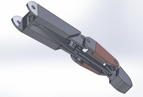
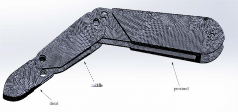
The finger designed for this study is illustrated in Figures 1 and 2. It consists of (3) phalanxes, (3) joints, (3) degrees of freedom and is powered by a servo motor that moves the two sets of links that embedded inside the finger. The first set of these links moves both the distal and middle phalanx and the second set moves the middle and proximal phalanxes. So the both of these sets connected together and operated by the servomotor in order to move the three phalanxes that finger consist of.
Figure 1. Structural arrangement for a finger
Figure 2. The three phalanxes of the finger
2.1 Forward kinematic analysis of the finger
The forward Kinematic mean find the position and orientation of the end effector relative to the base [11], so that a method of Denavit Hartenberg has been used, Denavit and Hartenberg notation provides a standardized method for writing kinematic equations of a manipulator. This is particularly useful for serial manipulators where a matrix is used to describe the posture (position and orientation) of one body relative to another. This method will depend on a set of parameters by which the relationship between the location of each phalange and the angle of each joint can be determined. The index finger will be taken as an example of forward kinematics analysis by finding the (Homogenous Transformation Matrix) and finding the Jacobin matrix, and the resulting equations have been theoretically verified by the MATLAB.
2.1.1 Denavit and Hartenberg frame
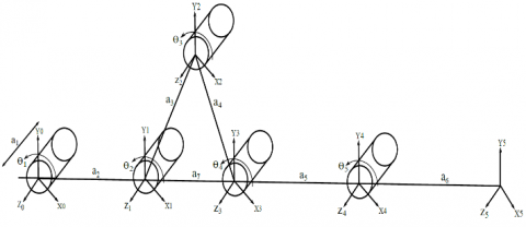
The kinematic diagram is shown in Figure 3, where the joints used in the designer finger are (revolt), and show how they connect to the links of the index finger, and was the determination of the Frames according to the method of (D. H). When the (O0) represents the center of the base of the finger and (Ot) represents the center of the fingertip.
Figure 3. The kinetic diagram of the embedded link in the finger
2.1.2 Denavit and Hartenberg parameter
Table 1 shows the parameters, since the number of rows will follow this equation:
No. of rows = No. of frame-1
Table 1. The D.H parameters for the finger
|
Frame |
θ |
α |
r |
d |
|
1 |
0+ θ1 |
0 |
a2 |
a1 |
|
2 |
0+ θ2 |
0 |
a7 |
0 |
|
3 |
0+ θ3 |
0 |
a8 |
0 |
|
4 |
0+ θ4 |
0 |
a5 |
0 |
|
5 |
θ5 |
0 |
a6 |
0 |
The number of columns in Table 1 is constant and is always (4) columns, since two of these parameters for a method (D.H) represent the rotations and are denoted by the (α) and (θ) symbols and the other two are the linear displacement and are coded by the symbols (d) and (r).
3.1 Forward kinematic for the index finger
As per Table 1. And concluded parameters of (D.H) method, it is possible to find (Homogenous Transformation Matrix) between each two adjacent links to reach to the (H.T.M) which connects the finger base links to its tip and as shown in Eq. (1).
Hn−1n=[cθn−sθncαnsθnsαnrncθnsθncθncαn−cθnsαnrnsθn0sαncαndn0001] (1)
When (s) refer to (sin) and (c) refer to (cos), so to find (H.T.M) between the base of the finger and the tip of it, we must find H01,H12,H23,H34,H45.
When:
H05=H01⋅H12⋅H23⋅H34⋅H45 (2)
From Eq. (1). When (n=1),
H01=[cθ1−sθ10a2cθ1sθ1cθ10a2sθ1001a10001] (3)
For (n=2),
H12=[cθ2−sθ20a7cθ2sθ2cθ20a7sθ200100001] (4)
For (n=3),
H23=[cθ3−sθ30a8cθ3sθ3cθ30a8sθ300100001] (5)
For (n=4),
H34=[cθ4−sθ40a5cθ4sθ4cθ40a5sθ400100001] (6)
For (n=5),
H45=[cθ5−sθ50a6cθ5sθ5cθ50a6sθ500100001] (7)
when: α1,2,3,4,5=0,cα1,2,3,4,5=1,sα1,2,3,4,5=0,
From Eq. (2). We can get H05 :
H05=[A11−A120A14A21−A220A24001a10001] (8)
A11=(mcθ4+nsθ4)cθ5+(ncθ4−msθ4)sθ5
A21=(lcθ4+fsθ4)cθ5+(fcθ4−lsθ4)sθ5
A12=(mcθ4+nsθ4)sθ5−(ncθ4−msθ4)cθ5
A22=(lcθ4+fsθ4)sθ5+(fcθ4−lsθ4)cθ5
A14=ra6cθ5+ta6sθ5+g
A24=wa6cθ5+ya6sθ5+h
When:
m=(cθ1cθ2−sθ1sθ2)cθ3−(cθ1sθ2
+sθ1cθ2)sθ3
n=(sθ1sθ2−cθ1cθ2)sθ3−(cθ1sθ2
+sθ1cθ2)cθ3
l=(sθ1cθ2+cθ1sθ2)cθ3+(cθ1cθ2−sθ1sθ2)sθ3
f=(cθ1cθ2−sθ1sθ2)cθ3−(sθ1cθ2
+cθ1sθ2)sθ3
r=(mcθ4+nsθ4),t=(ncθ4−msθ4),
w=(lcθ4+fsθ4)y=(fcθ4−lsθ4),
g=(ma5cθ4+na5sθ4+A)
h=(la5cθ4+fa5sθ4+B)
A=(cθ1cθ2−sθ1sθ2)a8cθ3−(cθ1sθ2
+sθ1cθ2)a8sθ3+(a7cθ2cθ1
−a7sθ1sθ2+a2cθ1)
B=(sθ1cθ2+cθ1sθ2)a8cθ3+(cθ1cθ2
−sθ1sθ2)a8sθ3+(a7cθ2sθ1
+a7cθ1cθ2+a2sθ1)
3.2 The Jacobian matrix for the index finger
The [J] matrix was established for the determining the speed of the tip of the finger, since this matrix represents the relationship between the speed of the links and the speed of the top of the finger [10]; when the [J] matrix is:
[˙x˙y˙z˙ωx˙ωy˙ωz]=J[˙θ1⋮⋮⋮˙θn] (9)
When (θ) refer to the joint variable this is mean that the Jacobin matrix has (number of columns equal to number of joints in the manipulator), also the number of rows of the Jacobin matrix always =6; in this paper the design finger has (5) joints, so the [J] matrix will consist of (6) rows and (5) columns, and equal to the total number of joints when i= the joint no.
The [J] matrix consists of two parts, one for the linear velocity of the fingertip and another part of the rotational velocity of the fingertip as shown in the Eq. (10).
[J]=[JvJω] (10)
[Jv] Refer to the linear part; [Jω] Refer to the rotating part of the Jacobin matrix, we can get the linear and rotational relation of the revolute joint that used in the design finger from the Table 2 .
Table 2. Joint model formula
|
|
Prismatic |
Revolt |
|
Linear |
R0i−1[001] |
R0i−1[001]×(o0n−o0i−1) |
|
Rotational |
[000] |
R0i−1[001] |
Thus, the Jacobian matrix will be in the following form:
[J]=[Jv1Jv2Jv3Jv4Jv5Jω1Jω2Jω3Jω4Jω5] (11)
When:
Jv1=R00[001]×(o05−o00),
Jv2=R01[001]×(o05−o01)
Jv3=R02[001]×(o05−o02)
Jv4=R03[001]×(o05−o03)
Jv5=R04[001]×(o05−o04)
Jω1=R00[001],Jω2=R01[001],Jω3=R02[001]
Jω4=R03[001]Jω5=R04[001]
Compensation value of (R0i) refers to a rotational matrix of each joint that index finger consist of and it is meat the rotational of frame (0) to the frame (i), we can get it from a homogenous transformation matrix in the previous section, also compensation values of (O0i) that refers to the displacement vector from the center of the frame (0) to the center of the frame (i), So we can find the Jacobian matrix as equation below:
[˙x˙y˙z˙ωx˙ωy˙ωz]=[J11J12J13J14J15J21J22J23J24J2500000000000000011111][˙θ1˙θ2˙θ3˙θ4˙θ5˙θ6] (12)
when:
J11=−(wa6cθ5+ya6sθ5+h),
J12=−(wa6cθ5+ya6sθ5+h−a2sθ1)
J13=wa6cθ5+ya6sθ5+h−(a7cθ2sθ1
−a7cθ1sθ2+a2sθ1)
J14=−(wa6cθ5+ya6sθ5+h−B)
J15=la5cθ4+fa5sθ4+B−(wa6cθ5+ya6sθ5
+h)
J21=ra6cθ5+ta6sθ5+g
J22=ra6cθ5+ta6sθ5+g−a2cθ1
J23=ra6cθ5+ta6sθ5+g−(a7cθ2cθ1+
a7sθ2sθ1+a2cθ1)
J24=ra6cθ5+ta6sθ5+g−A
J25=ra6cθ5+ta6sθ5+g−(ma5cθ4+na5sθ4+A)
4.1 Results
After deriving the forward kinematics and Jacobian matrix of the prosthetic finger designed, we get the location (position and orientation) of the fingertip according to the angle at which the joints rotate. For instance, we take note of the last line of Jacobian matrix will be the following:
˙ωz=˙θ1+˙θ2+˙θ3+˙θ4+˙θ5+˙θ6
This indicates that the rotational velocity of the tip of the finger around the axis (Z) depends on the velocity of θ1,θ2,θ3,θ4,θ5,θ6 (Joints variable), and if we go back to (Kinetic Diagram) we'll find its true cause the tip of the finger can be rotated around the (Z) axis by affecting each of them. As for the equation: ˙ωy=0, this means that there is no rotational velocity of the tip of the finger towards the axis (Y), which is also true in principle, since each of the constituent joints of the designed finger is do not rotate about (Y) axis, its only rotate about (Z) axis. Thus, we can adopt the remaining results generated by the derivation of these matrices to determine the exact location of the fingertip and its velocity. This has been verified in the next section.
4.2 Discussion
In this paper, the theoretical results are compared with the MATLAB result as shown in Table 3.
The results of the simulation tasks for a prosthetic finger design were done by the Solidwork 2018 which compared with the theoretical results the fingertip in the desired direction through the rotation of the joint angle.
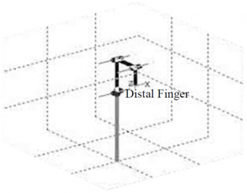
The MATLAB was used to verify the kinematic equations and matrices and to verify the path of movement of the index finger as shown in Figure 4. In order to achieve the similarity and conformity of the natural finger by inserting the values of the angles and lengths of the links those consist of the finger as shown in Table 3.
1. The convergence in the theoretical results data with the results extracted in MATLAB;
2. There is an agreement in the theoretical result with the result of MATLAB when the angles of joints of the finger is 90 degrees. The results are compatible with theoretical equations, the kinematic model and the Jacobin matrix, and the equations for the index finger are acceptable.
Table 3. The validation results of index finger forward kinematics
|
Variable joints |
Displacement fingertip (MATLB) |
Displacement finger tip (analysis) |
||||||||
|
\boldsymbol{\theta}_{1} |
\boldsymbol{\theta}_{2} |
\boldsymbol{\theta}_{3} |
\boldsymbol{\theta}_{4} |
\boldsymbol{\theta}_{5} |
X (mm) |
Y (mm) |
Z (mm) |
X (mm) |
Y (mm) |
Z (mm) |
|
90^{\circ} |
90^{\circ} |
90^{\circ} |
90^{\circ} |
90^{\circ} |
28 |
76 |
0 |
28 |
76 |
0 |
|
75^{\circ} |
75^{\circ} |
75^{\circ} |
75^{\circ} |
75^{\circ} |
43.655 |
35.417 |
0 |
44.555 |
33.89 |
0 |
|
15^{\circ} |
15^{\circ} |
15^{\circ} |
15^{\circ} |
15^{\circ} |
84.524 |
68.562 |
0 |
85.424 |
70.121 |
0 |
Figure 4. Simulation of forward Kinematics for the index finger
1. The observations made for motion in the current study of prosthetic finger and the links that consist of and compared and validated with theoretical and simulation in Table 3.
2. The designed index finger was shown to be capable of fulfilling functional requirements.
3. The solid work model can successively assist in studying the prosthetic finger, which can further assist in improving the design.
4. (3D) modeling can also assist the designing customized prosthetic hand for amputee efficiency and daily life tasks. However, more static and dynamic analysis must be carried out along with experimental validation for a comprehensive investigation.
[1] Chappell, P. (2016). Mechatronic hands prosthetic and robotic design. Institution of Engineering and Technology. https://doi.org/10.1049/PBCE105E
[2] Chen, D., Li, X., Jin, J., Ruan, C. (2019). An articulated finger driven by single-mode piezoelectric actuator for compact and high-precision robot hand. Review of Scientific Instruments, 90(1): 015003. https://doi.org/10.1063/1.5045817
[3] Moran, C.W. (2011). Revolutionizing prosthetics 2009 modular prosthetic limb-body interface: Overview of the prosthetic socket development. Johns Hopkins APL Technical Digest, 30(3): 250-255.
[4] El-Sheikh, M.A., Taher, M.F., Metwalli, S.M. (2012). New optimum humanoid hand design for prosthetic applications. The International Journal of Artificial Organs, 35(4): 251-262. https://doi.org/10.5301/ijao.5000067
[5] Quigley, M., Salisbury, C., Ng, A.Y., Salisbury, J.K. (2014). Mechatronic design of an integrated robotic hand. The International Journal of Robotics Research, 33(5): 706-720. https://doi.org/10.1177/0278364913515032
[6] Dave, A., Muthu, P., Karthikraj, V., Latha, S. (2018). Structural integration and control of peerless Human-like prosthetic hand. In Journal of Physics: Conference Series, 1000(1): 012066.
[7] Xu, K., Liu, H., Liu, Z., Du, Y., Zhu, X. (2015). A single-actuator prosthetic hand using a continuum differential mechanism. In 2015 IEEE International Conference on Robotics and Automation (ICRA), pp. 6457-6462. https://doi.org/10.1109/ICRA.2015.7140106
[8] Crawford, A.L., Perez-Gracia, A. (2010). Design of a robotic hand with a biologically-inspired parallel actuation system for prosthetic applications. In International Design Engineering Technical Conferences and Computers and Information in Engineering Conference, 44106: 29-36. https://doi.org/10.1115/DETC2010-28418
[9] Hovhannisyan, L., Davtyan, M., Hakobyan, A., Khanamiryan, Z. (2018). Original design, EMG controlled 3D simulation, and customization of a bionic hand. https://doi.org/10.13140/RG.2.2.26459.82721
[10] Ceccarelli, M. (2015). Finger mechanisms for robotic hands. Mach Sci, 33: 3-13. https://doi.org/10.1007/978-3-319-18126-4_1
[11] Siciliano, B., Khatib, O. (2008). Handbook of Robotics, Springer.https://link.springer.com/content/pdf/10.1007%2F978-3-540-30301-5.pdf.