Juan Gabriel Rueda-Bayona* | Laura Gil | Jose Manuel Calderón
© 2021 IIETA. This article is published by IIETA and is licensed under the CC BY 4.0 license (http://creativecommons.org/licenses/by/4.0/).
OPEN ACCESS
The high development of the offshore industry for supporting new marine and renewable energy projects requires a constant improvement of methods for structure designing. Because recent studies warned that maximum environmental loads occur during low sea states and not during extreme sea states as recommend by the offshore standards (e.g., RP 2AWSD-2014), this study used measured wave and current data for analyzing that warning. The Colombian Caribbean coast was selected as the study area, and in situ ADCP data combined with Reanalysis and numerical data was used for identifying proper sea states for the analysis. Then, two low and one extreme sea states were selected and their associated current profiles were extracted, for providing input data for Computational Fluid Dynamics (CFD) and Finite Element Method (FEM) simulations to evaluate the effect of the hydrodynamic forces over a floating structure. The results showed that low sea states generated maximum loads and rotations in the floating structure, and the extreme sea states caused high-frequency vibrations that could provoke structural dynamics problems such as failures due to fatigue or sudden collapse by resonance and amplification.
CFD, FEM, hydrodynamics, hydromechanics, offshore, TLP
The increasing interest in non-conventional renewable energies worldwide motivated several countries to develop technologies such as the offshore wind turbines [1]. These offshore projects require rigorous engineering designing because of the complex fluid-structure interactions (environmental loads) that face the wind turbine foundations, in this sense, subjective designs may put at risk their stability that would generate environmental and operational problems. The traditional designing guidelines for marine structures recommend characterizing the wave climate to identify the designing load from the extreme sea states [2-12].
The increasing interest in developing offshore wind turbines is evidenced in recent studies [13-18] validated the numerical modeling of a 1:40 scale model under different environmental loads in a wave flume, and Li et al. [19] studied the transient responses of a SPAR-type turbine when one of the mooring lines suddenly fractures under extreme sea states. Tian et al. [20] studied the optimization of offshore wind turbine anchors considering specific wave parameters for the environmental loads. Chuang et al. [21] investigated how the mean drift force of the wave and the slow drift load of the platform influenced the movements of a platform, and concluded that the average drift force and slow drift force moved the structure away along the direction of wave propagation.
The complex fluid-structure interactions of offshore foundations have been studied through numerical approaches (physical modeling), to understand how the hydrodynamic forces affect the dynamic and mechanical properties of diverse marine structures. Bruinsma et al. [22] analyzed the vertical movements of a moored floating structure through numerical modeling and compared the complex fluid-structure interactions against measured experimental results. Ishihara and Ishihara and Zhang [23] developed a non-linear simulation tool coupled to the Morrison equation to determine the dynamic response of a floating structure and concluded that the quasi-static model successfully reproduced the first three main displacements. Cheng et al. [24] performed CFD modeling of a floating offshore wind turbine through the OpenFOAM model, to analyze the fluid-structure interactions under several sea state conditions. Yue et al. [25] analyzed the hydromechanics of a Spar floating platform through the numerical model ANSYS-Aqwa, and Barooni et al. [26] and Sant et al. [27] used the same software to analyze the hydromechanics of an offshore wind turbine under different environmental loads.
However, Rueda-Bayona, J.G. et al. revised these guidelines and warned that extreme hydrodynamic forces did not occur during extreme sea states (high surface waves), but these extreme forces appeared during low sea states with wave height less than 1 m [28, 29]. The authors recommended inspecting low sea states for identifying extreme hydrodynamic forces when the offshore foundation is under an inertia regime [30], which is the most common regime for offshore wind turbine: water depth > 30 m, wave heights > 1 m, and wave period higher than 4 s. Also, the literature review performed by Rueda-Bayona, J.G. et al. [28, 29] showed that several studies considered the standard guidelines for analyzing the structural dynamics of offshore structures, then, those studies omitted that during low sea-states a non-uniform current profile may generate higher hydrodynamic forces than can produce high waves during extreme sea-states such as hurricanes or cold fronts.
The revised literature showed that offshore designing may be excluding extreme hydrodynamic forces during low sea-states because of the standards recommendation of selecting environmental design loads from extreme sea-states. Hence, this study used measured current profiles during low and extreme sea-states to verify if maximum hydrodynamic forces may occur under low sea-states as warned [28, 29], and analyze the effect of the hydrodynamic forces over the mechanical and dynamic properties of a Tension-leg Platform (TLP). The CFD-FEM modeling of this study provides more evidence that low-sea states may generate critical structural responses, because current profiles may generate higher hydrodynamic forces than extreme waves if the offshore structure is in an inertia regime.
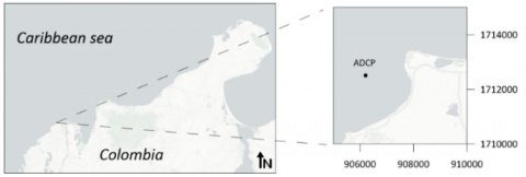
This research comprises 3 main sections: 1- hydrodynamics, 2-Structural mechanics, and 3-hydromechanics. After defining the study area, was necessary in situ ocean data to identify low and extreme sea states for the current profile selection. The study case was performed in the Colombian Caribbean coast where the in-situ data was retrieved from the study of Rueda Bayona [31, 32], who used measured data from an Acoustic Doppler Current Profiler (ADCP) located in 11.038° N 74.943° W (Figure 1). The ADCP measured at 8 m water-depth and recorded wave and current data from June 3rd to December 11th of 2015 with 10 minutes of interval.
Figure 1. Study area and location of the in situ current profiles measured by ADCP. Coordinates in Magna Sirgas (Bogotá zone)
The surface wind data was downloaded and processed from the NARR-NOAA database [33] which has a 3-hourly time interval of frequency. The water level data was generated through the hydrodynamic Delft3D model which was previously implemented and calibrated by Rueda-Bayona et al. [34].
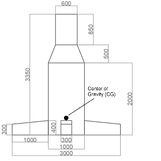
The characteristics of the control volume, the foundation location, and the selected layers (planes) for the CFD analysis are depicted in Figure 2a. The TLP (Figure 2b) was perfectly fixed into the seafloor to analyze the effect of currents over the near hydrodynamic field of a non-mobile solid, and how the hydrodynamic forces affect the main mechanical properties of the foundation such as the Von Misses stress.
The CFD (Computational Fluid Dynamics) and FEM (Finite Element Method) were performed through the ANSYS software V.2019 R2 (www.ansys.com), which is a multiphysics numerical model able to simulate complex fluid-structure interactions and other physical problems [35-37]. The numerical strategy to simulate the effects of the extreme current profiles (Figure 6) over the TLP (Figure 2) is shown in Figure 3, where the CFD analysis will be done by the Fluent model (Fluid Flow) known as Ansys-Fluent, and the FEM through the structural model (Static structural) known as Ansys-Mechanical. The Ansys-Fluent solves the Reynold Averaged Navier-Stokes (RANS) equations for computing properties of the hydrodynamic field (velocities, pressures, forces, and turbulent parameters), and the Ansys-Mechanical uses the hydrodynamic data generated by Ansys-Fluent to calculate deformations and mechanical parameters of the solid body.
(a)
(b)
Figure 2. (a) Numerical control volume and plane views of TLP for the CFD modeling, (b) main dimensions of TLP foundation; units in millimeters
Figure 3. Structure of the numerical approach and data pathlines for the CFD-FEM simulations in the ANSYS Workbench
The properties and boundary conditions of the CFD model are seen in Table 1, such as the fluid control volume characteristics and the applied numerical methods. The fluid properties listed in Table 1 were taken from the seawater characteristics reported for the study area [31, 34] and the Steel density was selected considering common mechanical parameters for offshore structures used by Rueda-Bayona et al. [28]. The Boundary conditions considered an upstream magnitude field normal to the boundary which generated a resultant hydrodynamic field according to the expected fluid-structure interaction [29].
The solution methods, spatial discretization and turbulence parameters were tuned considering the convergence of the numerical solution, the expected behavior of the hydrodynamic field perturbed by a monopile [38, 39] and by the shape of the current field nearby to the study area [28, 31, 32, 40]. The pressure-based solver was selected to perform a pressure correction that enhanced the numerical stability, and the model was run in stationary mode because it showed better stability than transient mode.
The mechanical properties of the TLP foundation such as the Isotropic Elasticity derived from Young's Modulus and Poisson's Ratio are listed in Table 2.
Table 1. Fluid properties, boundary conditions, and numerical approach of the CFD model (ANSYS-Fluent)
|
Parameter |
Value |
|
Seawater density (kg/m3) |
1020 |
|
Viscosity (kg/m*s) |
0.0002 |
|
Solver |
pressure based |
|
Velocity formulation |
absolute |
|
Time |
steady |
|
Z gravity (m/s2) |
-9.81 |
|
Steel density (kg/m3) - solid |
7850 |
|
Boundary conditions |
upstream |
|
Velocity specification method |
magnitude, normal to the boundary |
|
Reference frame |
absolute |
|
Turbulence - method |
Intensity and viscosity ratio |
|
Turbulent intensity (%) |
5 |
|
Turbulent viscosity ratio |
10 |
|
Solution methods |
|
|
Pressure-velocity coupling |
Yes |
|
Scheme |
coupled |
|
Spatial discretization |
|
|
Gradient |
Least Squares Cell-based |
|
Pressure |
Second-order |
|
Momentum |
Second-order Upwind |
|
Turbulent Kinetic Energy |
1st order upwind |
|
Specific dissipation rate |
1st order upwind |
|
Pseudo transient |
yes |
|
Pressure |
0.5 |
|
Momentum |
0.5 |
|
Density |
1 |
|
Body forces |
1 |
|
Turbulent Kinetic Energy |
0.75 |
|
Specific dissipation rate |
0.75 |
|
Turbulent viscosity |
1 |
Table 2. Mechanical properties of the TLP foundation for the FEM through ANSYS-Mechanical
|
Parameters |
value |
|
Young's modulus (MPa) |
200000 |
|
Poisson's ratio |
0.3 |
|
Bulk modulus (MPa) |
167000 |
|
Shear modulus (MPa) |
76900 |
|
Isotropic Secant Coefficient of Thermal Expansion 1/°C |
0.000012 |
|
Compressive Ultimate Strength (MPa) |
0 |
|
Compressive Yield Strength (MPa) |
250 |
|
Tensile Ultimate Strength (MPa) |
460 |
|
Tensile Yield Strength (MPa) |
250 |
Figure 4 depicts the applied scheme for modeling the hydromechanics parameters of the TLP such as rotation, displacements, and acceleration, through the Aqwa module of ANSYS; The Aqwa module is a 3D diffraction/radiation model to analyze the effect of waves, wind, and currents over marine structures [41]. It was necessary to calculate the Gamma parameter to define the JONSWAP spectrum required by the Aqwa module, hence, it was applied a Genetic Algorithm model (GA) developed by the Ref. [40] for finding a proper Gamma value; details of the GA model fundamentals and its applications may be found in the work of [32, 40, 42]; the boundary conditions and configuration of the Aqwa module are described in Table 3.
Figure 4. Structure of the numerical approach and data pathlines in the ANSYS Workbench for the Aqwa module
Table 3. Fluid properties, boundary conditions, and numerical approach of the CFD model (ANSYS-Aqwa)
|
Parameter |
value |
|
Seawater density (kg/m3) |
1020 |
|
Water depth (m) |
8 |
|
Water size x, y (m) |
16, 16 |
|
Total mass (kg) |
2169 |
|
CG (m) |
-2.014 |
|
Momment of inertia Ixx, Iyy, Izz (kg*m^2) |
740, 740, 395.5 |
|
z gravity |
-9.81 |
|
Connection point for riser |
4 |
|
Analysis setting |
Time Response Analysis |
|
Analysis type |
Irregular wave response |
|
Time step (s) |
0.0005 |
|
Time interval (s) |
120 |
|
Wave type |
JONSWAP |
|
Gamma |
3.5, 8.53, 1.75 |
|
Current profile type |
Varies with depth |
|
Use cable dynamics |
yes |
Note: CG is the gravity center, the Gamma values correspond to the three analyzed sea states.
Table 4. Mechanical properties of riser for TLP foundation ANSYS-Aqwa
|
Parameters |
Value |
|
Material type |
HMPE |
|
Riser density (kg/m^3) |
865 |
|
Young's Modulus (MPa) |
140000 |
|
Diameter (mm) |
120 |
|
Length (m) |
5.5 |
|
Axial stiffness (N/mm) |
287884 |
The selected material for the mooring lines of TLP was the high modulus polyethylene (HMPE), which is commonly used for permanent mooring lines; the polyester and aramid materials were previously evaluated but they were discarded because HMPE outperformed them when restricting TLP movements. The HMPE is considered a promising synthetic fiber for future applications in the offshore industry due to its high rigidity [43], also, Ikhennicheu et al. [44] mentioned that HMPE has a high resistance against abrasion and tension compared to other synthetic fibers. The properties of the HMPE mooring lines are described in Table 4.
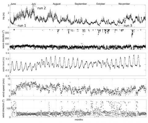
The identification of the low and extreme sea states of the study area considered the climate analysis performed by previous studies, which pointed to a low sea state when significant wave heights (Hs) are below 1.28 m, and an extreme sea state occurs when Hs is higher than 2.87 m [40]. In this sense, the evolution of significant wave heights (Hs) allowed identifying 3 sea states (Figure 5), pointed as run 1, 2, and 3, which 2 of them (run 1 and 3) occurred during a low sea state, and run 2 showed an extreme sea state. Considering that winds and water level induce the generation of extreme hydrodynamic forces [28], the evolution of these parameters were plotted together with the Hs and wave direction (Figure 5); waves and winds have an oceanographic convention, winds come from and waves go to.
From the 3 sea states were selected 3 current profiles, each of them associated with an extreme and low sea state (Table 5). The measured current profiles have 0.4 m of cell size with 0.4 m of blanking, what represent 20 measurement points alongside the 8 m of water column (Figure 6).
Figure 5. Oceanographic data from June 3rd to December 12th of 2015. The ADCP wave time series and 10-m wind data of the study area were edited from the Ref. [31]
Table 5. Oceanographic parameters of the 3 selected ADCP current profiles
|
Date - time |
Hs (m) |
Tp (s) |
Wave direction (°) |
Wind speed (m/s) |
Wind direction (°) |
Sea-state |
Tide condition |
Run |
|
|
June |
3/06/2015 -10:00 |
0.44 |
7.76 |
56 |
2.40 |
50 |
low |
Ebb |
1 |
|
July |
4/07/2015 - 2:00 |
3.06 |
10.78 |
60 |
11 |
33 |
extreme |
Ebb |
2 |
|
October |
15/10/2015 -3:00 |
0.3413 |
6.92 |
30 |
5.82 |
31 |
low |
Ebb |
3 |
Figure 6. ADCP current velocity profile
The CFD analysis of the TLP foundations considered the effect of the nearby hydrodynamic field over the structure and the structural-hydromechanic responses. Accordingly, in the next sections, were evaluated the hydrodynamics around the TLP and the effect of hydrodynamic forces over the mechanical and hydromechanics properties.
3.1 Hydrodynamics
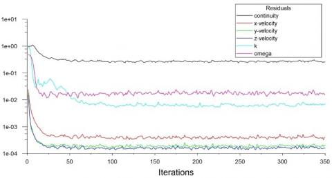
The hydrodynamic analysis required a previous inspection of numerical residuals to guarantee the quality of the CFD modeling. As a result, the residuals were close to 0 and kept stable evidencing that the model generated good results because it reached the numerical convergence (Figure 7).
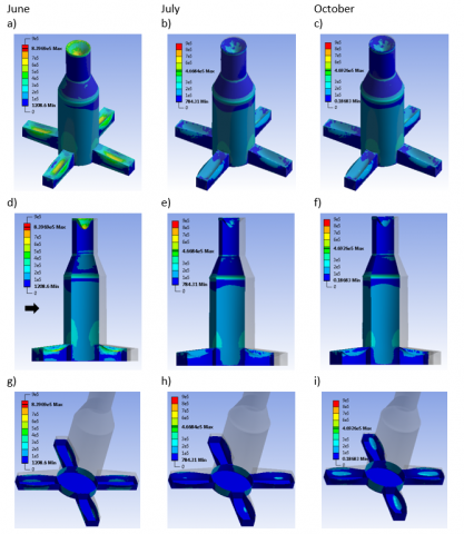
The Figure 8 shows that the maximum velocity field occurred during the low sea states (Hs < 0.5 m) of June and October, then, the maximum hydrodynamic forces were generated during these events. The maximum current velocities were observed in June (Figure 8a, d, g) with values about 1 m/s nearby to the TLP legs, followed by the results of October which not exceeded the 0.9 m/s in the upper planes of the hydrodynamic fields (Figure 8f, i).
The results of July showed that current velocities were not higher than 0.7 m/s (Figure 8b, e, h), evidencing that the maximum velocities did not occur during the extreme sea state of this month (Table 5). The current velocities in Figure 8 were similar to the measured in Ref. [31], where low sea states showed maximum current profiles. The streamlines generated by the CFD modeling showed the hydrodynamic behavior for the 3 sea states (Figure 9), which showed the stagnation zones and the maximum velocities reported in the low sea states of June and October (Figure 8). According to the subcritical regime of Reynolds number (Re=2500), the Keulegan-Carpenter number (KC = 9), and the behavior of streamlines, there were not evidenced of vortex around the TLP.
3.2 Structural mechanics
To identify the effect of the measured current profiles over the TLP during the low and extreme sea states of the study area (Table 5), the hydrodynamic results of the Ansys-Fluent model were transferred to the Ansys-Mechanical model (Figure 3) in terms of hydrodynamic loads. The FEM performed by the Mechanical-Ansys module pointed that the maximum stress occurred during June with a value of 8.3969 x 10⁵ Pa (Figure 10 a, d), where the maximum stresses appeared at the top of the cylinder section (600 m of diameter) (Figure 2b) and at the 4 TLP legs; the minimum Von Mises stress was 0.1868 Pa occurred in October (Figure 10 c, f, i).
Figure 7. Residual information of run convergence of ANSYS-Fluent module
Figure 8. Velocity contours generated by the current velocity profiles during extreme and low sea states occurred in June, July, and October of 2015; the black arrow represents the upstream flow
Figure 9. Streamlines generated by the current velocity profiles during extreme and low sea states occurred in June, July, and October of 2015; the black arrow represents the upstream flow
Figure 10. Von Mises stress (Pa) generated by the current velocity profiles during extreme and low sea states occurred in June, July, and October of 2015; the black arrow represents the upstream flow
The maximum stress of the TLP foundation generated by the current profiles of June, July, and October showed similar values (0.84 MPa) to the Ref. [28] (1.95 MPa). That study evaluated an offshore monopile located in the same region (Colombian Caribbean coast) and considered similar environmental loads, sea states, and materials. Also, similar to our research that study reported that the maximum hydrodynamic force occurred during a low sea state with a wave height < 0.7 m and a wind speed < 4 m/s.
The isobaths and coastline orientation of this study were also similar to the study [28], as well as the wind characteristics, however, the wave direction of this study was different because the waves propagated to the east due to the wave-refraction generated by the water depth reduction nearby to the shore. Due to the waves of that study propagated to the south-east and the flood tide was starting, those forcers eased the water flux development provoking the maximum hydrodynamic forces. In this study, the ebb tide was at the half period where the maximum accelerations occurred. As a result, the maximum currents of the ebb tide combined with a low sea state and winds blowing from the east (30°-50°), eased the increment of current velocities in the profiles of June and October (run 1 and 3) (Figure 6). The current profile of July showed the lowest magnitudes because the potential energy of its high waves reduced the kinetic energy at the surface. The study area of this research is influenced by the surface river plume of Magdalena River [31, 34, 45], then, the plume effect over the currents field, combined with the ebb tide, winds from the northeast, and low wave heights, generated the maximum hydrodynamic forces.
3.3 Hydromechanics
The dynamic behavior of the TLP was analyzed through the hydromechanic module of ANSYS (Aqwa). The numerical results of Aqwa pointed that the maximum displacements (2.8 m, sway) occurred in July, higher than observed in June and October which reported displacements (sway) of 1.2 m and 0.8 m respectively Figure 11. The extreme sea state of July was characterized by Hs = 3.06 m and Tp = 10.78 s (Table 5), which excited the TLP with high energy and provoked the high sway and surge movements.
Figure 11. TLP Displacements during extreme and low sea states occurred in June, July, and October of 2015
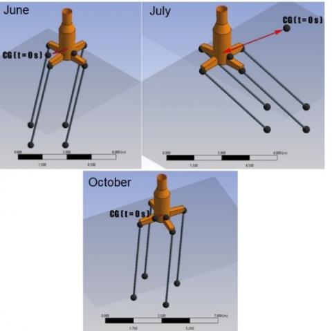
The TLP displacement from the initial center of gravity (CG) was simulated by the Aqwa module for all the three sea states (Table 5). The initial position started at the beginning of the simulation of each run (t= 0 s), then, after several time steps the TLP was excited due to the effect of ocean waves and current profile defined in the boundary conditions of each run (Table 5, Figure 6)
The numerical results retrieved from Aqwa pointed that July showed the maximum 3D resultant displacement of CG (3.762 m), what means the final position of the CG in the 3-dimensional space. In addition, July reported a maximum downward displacement of -1.29 m (z, vertical) and the maximum horizontal displacement (x,y) of -2.152 m and -2.805 m respectively, which correspond to the surge and sway TLP movements. The Figure 12 shows the 3D resultant displacement of CG, where the run of July evidenced the TLP movement and mooring lines inclination because of the effect of the extreme sea state (Figure 12).
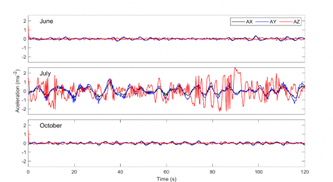
The structural dynamic response of the TLP was analyzed using the acceleration results of the TLP. As a result, the structure presented maximum accelerations of 2.5 m/s2 in July, higher compared to the results of June and October with maximum accelerations of 0.5 m/s2 (Figure 13); the highest accelerations of July occurred at the time step of 90 s, the same instant when a maximum surge and sway displacement were reported (Figure 11).
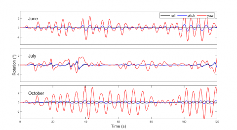
The rotational displacements of TLP during the low and extreme sea states are plotted in Figure 14. The maximum rotations for all the 3 runs were yaw, due to the loads impact over the TLP surface area provoked rotational movements around the z vertical axis in the structure. The structure presents rotations not greater than 4 degrees approximately for each of the sea states. The greatest rotations occurred in the time instant of 40 s belonging to July. The maximum gyre in yaw occurred in October (3.63°), followed by June (3.09°) and July (1.75°).
Table 6. Maximum displacement of the center of gravity (CG) of TLP
|
CG Location |
Modeling time (s) |
Horizontal axis |
Vertical axis |
3D Resultant displacement (m) |
|
|
x (m) |
y (m) |
z (m) |
|||
|
Initial |
0 |
0 |
0 |
-2.014 |
0 |
|
June (Final) |
38.75 |
0.183 |
1.451 |
-2.212 |
1.476 |
|
July (Final) |
35.5 |
-2.152 |
-2.805 |
-3.301 |
3.762 |
|
October (Final) |
6.5 |
-0.438 |
0.687 |
-2.075 |
0.817 |
Figure 12. 3D Resultant displacement of TLP during each sea state
According to the results of TLP displacements, was observed that low sea states of June and October caused more horizontal displacement than July’s extreme sea state. The sway displacement kept positive (0.5 m to 1 m) for June and October, hence, the high surface current velocities (0.7 m/s to 0.9 m/s) seen in Figure 6 provoked a net thrust over the TLP what generated the permanent positive sway. During July, the lateral movements of surge and sway were controlled by the predominant waves which moved the CG to a 3D resultant displacement of 3.762 m (Table 6).
The CFD-FEM results of the TLP in this study revealed that low sea states comprise high current velocities and extreme hydrodynamic forces that affect the stability and stress of the structure. When low Hs < 0.5 m and Peak period (Tp) < 8 s combined with high surface currents (velocity > 0.7 m/s), high extreme hydrodynamic forces were generated, similar to the findings [28]. As a result, maximum Von Mises stress and the highest rotational movements around the vertical axis occurred in June and October. During the extreme sea state of July, characterized by a high Hs > 3 m and Peak period (Tp) > 10 s combined with low surface currents (velocity < 0.3 m/s) caused the highest sway and heave displacements as well as the highest accelerations in the TLP.
The comparison of CFD-FEA results between low and extreme sea states revealed that in low sea states predominated the inertia forces that provoked higher loads over the TLP and high rotation around the vertical axis, and during extreme sea states caused the highest vibrations because the accelerations exceeded the 2 m/s2. Accordingly, during the offshore structure design, not only the low sea states must be considered for identifying maximum loads and rotations of floating structures, but also the extreme sea states because they will provide information of vibrations with high frequency that could provoke structural problems related to resonance, fatigue, and structural amplifications. There exist several studies which analyzed numerically [46-48] and experimentally [49] the effect of extreme sea states over the hydromechanics of offshore structures (e.g floating wind turbines), but the important effect of low sea states over the structural behaviour warned by Rueda-Bayona et al. [28] have not been wide documented.
Figure 13. Accelerations components (x,y,z) of the structure during extreme and low sea states occurred in June, July, and October of 2015
Figure 14. Rotations of the structure during extreme and low sea states occurred in June, July, and October of 2015
The offshore structure design considers that maximum hydrodynamic forces appear during extreme sea states (highest wave height), in this sense, the standards and guidelines suggest selecting the wave parameters of these extreme events for estimating the environmental loads. Considering that recent studies that utilized numerical modeling reported that maximum hydrodynamic forces occurred during low sea states, this study used measured wave and current data for validating if maximum hydrodynamic forces may occur during low sea states.
As a result, 3 sea states were analyzed in the Colombian Caribbean Coast, and their associated current profiles were extracted for the analysis. The current profiles of June, July, and October of 2015 were used to perform CFD-FEM simulations of a TLP. The results evidenced that maximum Von Misses stress appeared in June during a low sea state, and not during July, where the maximum wave heights were 3 m.
Then, the results of [28] reporting that low sea states generate higher hydrodynamic forces than extreme sea states were confirmed by this study. Also, this study agreed with [28] which suggested that the increment of hydrodynamic forces depends on the wind-wave-tides interactions and by the geomorphological and bathymetry characteristics. Then, this research evidenced that Ebb tides during a low sea state (Hs < 0.5 m), wind speed less than 4 m/s blowing from the northeast, generated maximum hydrodynamic forces at the study area.
As future research it is recommended to analyze low sea states in different regions with higher latitudes, to confirm the applicability of selecting low sea states for identifying extreme hydrodynamic forces.
This work was supported by the Universidad Militar Nueva Granada (project IMP-ING-3121).
[1] Rueda-Bayona, J.G., Guzmán, A., Eras, J.J.C., Silva-Casarín, R., Bastidas-Arteaga, E., Horrillo-Caraballo, J. (2019). Renewables energies in Colombia and the opportunity for the offshore wind technology. Journal of Cleaner Production, 220: 529-543. https://doi.org/10.1016/j.jclepro.2019.02.174
[2] American Petroleum Institute. Production Department. (2013). Recommended Practice for Design and Hazards Analysis for Offshore Production Facilities.
[3] API. (2007). API BULL 2INT-DG: Interim Guidance for Design of Offshore Structures for Hurricane Conditions. https://standards.globalspec.com/std/1010996/api-bull-2int-dg.
[4] NORSOK. (2017). NORSOK N-003:2017. Actions and actions effects, 3rd ed. Norway. http://www.standard.no/en/nyheter/nyhetsarkiv/petroleum/2017-news/new-edition-of-norsok-n-003-actions-and-actions-effects/#.W2cnnihKjDc.
[5] API. (2011). API RP 2FPS: Recommended Practice for Planning, Designing, and Constructing Floating Production Systems, 2nd ed. https://global.ihs.com/doc_detail.cfm?document_name=API RP 2FPS.
[6] API. (2007). Recommended Practice for Planning, Designing and Constructing Fixed Offshore Platforms — Working Stress Design, Api Recomm. Pract. 24-WSD 242. https://doi.org/10.1007/s13398-014-0173-7.2
[7] International Electrotechnical Commission, IEC. (2009). 61400-3 Ed. 1.0 b:2009: Wind turbines - Part 3: Design requirements for offshore wind turbines. https://webstore.iec.ch/publication/5446.
[8] British Standard. (2008). BS EN ISO 19902:2007+A1:2013: Petroleum and natural gas industries. Fixed steel offshore structures, 1st ed. https://www.iso.org/standard/27507.html
[9] International Organization for Standardization. (2013). ISO 19900:2013: Petroleum and natural gas industries - General requirements for offshore structures. International Organization for Standardization. https://www.iso.org/standard/59877.html.
[10] International Organization for Standardization (2015) ISO 19901-1:2015: Petroleum and natural gas industries - Specific requirements for offshore structures - Part 1: Metocean design and operating considerations. https://www.iso.org/standard/34586.html.
[11] British Standard. (2015). BS ISO 29400:2015: Ships and marine technology - Offshore wind energy - Port and marine operations. https://www.iso.org/standard/60906.html.
[12] DNV, G. (2014). DNV-OS-J101–Design of offshore wind turbine structures. DNV GL: Oslo, Norway.
[13] Pham, T.D., Shin, H. (2019). Validation of a 750 kW semi-submersible floating offshore wind turbine numerical model with model test data, part I: Model-I. International Journal of Naval Architecture and Ocean Engineering, 11(2): 980-992. https://doi.org/10.1016/j.ijnaoe.2019.04.005
[14] Dai, J., Hu, W., Yang, X., Yang, S. (2018). Modeling and investigation of load and motion characteristics of offshore floating wind turbines. Ocean Engineering, 159: 187-200. https://doi.org/10.1016/j.oceaneng.2018.04.003
[15] Sarkar, S., Chen, L., Fitzgerald, B., Basu, B. (2020). Multi-resolution wavelet pitch controller for spar-type floating offshore wind turbines including wave-current interactions. Journal of Sound and Vibration, 470: 115170. https://doi.org/10.1016/j.jsv.2020.115170
[16] Chen, L., Basu, B., Nielsen, S.R. (2018). A coupled finite difference mooring dynamics model for floating offshore wind turbine analysis. Ocean Engineering, 162: 304-315. https://doi.org/10.1016/j.oceaneng.2018.05.001
[17] Manikandan, R., Saha, N. (2019). Dynamic modelling and non-linear control of TLP supported offshore wind turbine under environmental loads. Marine Structures, 64: 263-294. https://doi.org/10.1016/j.marstruc.2018.10.014
[18] Kim, J., Shin, H. (2020). Validation of a 750 kW semi-submersible floating offshore wind turbine numerical model with model test data, part II: Model-II. International Journal of Naval Architecture and Ocean Engineering, 12: 213-225. https://doi.org/10.1016/j.ijnaoe.2019.07.004
[19] Li, Y., Zhu, Q., Liu, L., Tang, Y. (2018). Transient response of a SPAR-type floating offshore wind turbine with fractured mooring lines. Renewable Energy, 122: 576-588. https://doi.org/10.1016/j.renene.2018.01.067
[20] Tian, Y.H., Gaudin, C., Randolph, M.F., Cassidy, M.J., Peng, B. (2018). Numerical investigation of diving potential and optimization of offshore anchors. American Society of Civil Engineers, 144(2): 1-9. https://doi.org/10.1061/(ASCE)GT.1943-5606.0001830
[21] Chuang, Z., Liu, S., Lu, Y. (2020). Influence of second order wave excitation loads on coupled response of an offshore floating wind turbine. International Journal of Naval Architecture and Ocean Engineering, 12: 367-375. https://doi.org/10.1016/j.ijnaoe.2020.01.003
[22] Bruinsma, N., Paulsen, B.T., Jacobsen, N.G. (2018). Validation and application of a fully nonlinear numerical wave tank for simulating floating offshore wind turbines. Ocean Engineering, 147: 647-658. https://doi.org/10.1016/j.oceaneng.2017.09.054
[23] Ishihara, T., Zhang, S. (2019). Prediction of dynamic response of semi-submersible floating offshore wind turbine using augmented Morison's equation with frequency dependent hydrodynamic coefficients. Renewable Energy, 131: 1186-1207. https://doi.org/10.1016/j.renene.2018.08.042
[24] Cheng, P., Huang, Y., Wan, D. (2019). A numerical model for fully coupled aero-hydrodynamic analysis of floating offshore wind turbine. Ocean Engineering, 173: 183-196. https://doi.org/10.1016/j.oceaneng.2018.12.021
[25] Yue, M., Liu, Q., Li, C., Ding, Q., Cheng, S., Zhu, H. (2020). Effects of heave plate on dynamic response of floating wind turbine Spar platform under the coupling effect of wind and wave. Ocean Engineering, 201: 107103. https://doi.org/10.1016/j.oceaneng.2020.107103
[26] Barooni, M., Ali, N.A., Ashuri, T. (2018). An open-source comprehensive numerical model for dynamic response and loads analysis of floating offshore wind turbines. Energy, 154: 442-454. https://doi.org/10.1016/j.energy.2018.04.163
[27] Sant, T., Buhagiar, D., Farrugia, R.N. (2018). Evaluating a new concept to integrate compressed air energy storage in spar-type floating offshore wind turbine structures. Ocean Engineering, 166: 232-241. https://doi.org/10.1016/j.oceaneng.2018.08.017
[28] Rueda-Bayona, J.G., Fernando Osorio-Arias, A., Guzmán, A., Rivillas-Ospina, G. (2019). Alternative method to determine extreme hydrodynamic forces with data limitations for offshore engineering. Journal of Waterway, Port, Coastal, and Ocean Engineering, 145(2): 05018010. https://doi.org/10.1061/(ASCE)WW.1943-5460.0000499
[29] Rueda-Bayona, J.G. (2015). Caracterización hidromecánica de plataformas marinas en aguas intermedias sometidas a cargas de oleaje y corriente mediante modelación numérica. Escuela de Geociencias. http://www.bdigital.unal.edu.co/51624/.
[30] Chakrabarti, S. (2005). Handbook of Offshore Engineering (2-volume set). Elsevier.
[31] Rueda-Bayona, J.G. (2017). Identificación de la influencia de las variaciones convectivas en la generación de cargas transitorias y su efecto hidromecánico en las estructuras Offshore. http://manglar.uninorte.edu.co/bitstream/handle/10584/7629/juanrueda.pdf?sequence=1&isAllowed=y.
[32] Rueda-Bayona, J.G., Guzmán, A., Silva, R. (2020). Genetic algorithms to determine JONSWAP spectra parameters. Ocean Dynamics, 70(4), 561-571. https://doi.org/10.1007/s10236-019-01341-8
[33] NOAA. (2016). NCEP North American Regional Reanalysis: NARR.
[34] Rueda-Bayona, J.G., Horrillo-Caraballo, J., Chaparro, T.R. (2020). Modelling of surface river plume using set-up and input data files of Delft-3D model. Data in Brief, 31: 105899. https://doi.org/10.1016/j.dib.2020.105899
[35] Emani, S., Yusoh, N.A., Gounder, R.M., Shaari, K.Z. (2017). Effect of operating conditions on crude oil fouling through CFD simulations. International Journal of Heat and Technology, 35(4), 1034-1044. https://doi.org/10.18280/ijht.350440
[36] Chen, B. (2018). Finite element strength reduction analysis on slope stability based on ANSYS. Environmental and Earth Sciences Research Journal, 4(3): 60-65. https://doi.org/10.18280/eesrj.040302
[37] Sharma, M., Soni, M. (2021). A finite element modeling and simulation of human temporomandibular joint with and without tm disorders: An Indian experience. Mathematical Modelling, 8(3): 347-355. https://doi.org/10.18280/mmep.080303
[38] Sarpkaya, T. (1993). Offshore hydrodynamics. Journal of Offshore Mechanics and Arctic Engineering, 115(1): 2-5. https://doi.org/10.1115/1.2920085
[39] Journée, J.M.J., Massie, W.W. (2002). Offshore Hydromechanics. https://ocw.tudelft.nl/wp-content/uploads/OffshoreHydromechanics_Journee_Massie.pdf.
[40] Rueda-Bayona, J.G., Guzmán, A., Cabello Eras, J.J. (2020). Selection of JONSWAP spectra parameters during water-depth and sea-state transitions. Journal of Waterway, Port, Coastal, and Ocean Engineering, 146(6): 04020038. https://doi.org/10.1061/(ASCE)WW.1943-5460.0000601
[41] ANSYS Inc. (2012). AQWA Reference Manual, Ansys. 15317. https://cyberships.files.wordpress.com/2014/01/aqwa_ref.pdf.
[42] Rueda-Bayona, J.G., Guzmán, A. (2020). Genetic algorithms to solve the jonswap spectra for offshore structure designing. In Offshore Technology Conference, Houston, Texas, USA. https://doi.org/10.4043/30629-ms
[43] Cruz, J., Atcheson, M. (2016). Floating Offshore Wind Energy. Springer. https://doi.org/https://doi.org/10.1007/978-3-319-29398-1
[44] Ikhennicheu, M., Lynch, M., Doole, S., et al. (2021). Review of the state of the art of mooring and anchoring designs, technical challenges and identification of relevant DLCs. https://corewind.eu/wp-content/uploads/files/publications/COREWIND-D2.1-Review-of-the-state-of-the-art-of-mooring-and-anchoring-designs.pdf.
[45] Alvarez-Silva, O., Osorio, A.F. (2015). Salinity gradient energy potential in Colombia considering site specific constraints. Renewable Energy, 74: 737-748. https://doi.org/10.1016/j.renene.2014.08.074
[46] Li, H., Díaz, H., Soares, C.G. (2021). A failure analysis of floating offshore wind turbines using AHP-FMEA methodology. Ocean Engineering, 234: 109261. https://doi.org/10.1016/j.oceaneng.2021.109261
[47] Qu, X., Li, Y., Tang, Y., Hu, Z., Zhang, P., Yin, T. (2020). Dynamic response of spar-type floating offshore wind turbine in freak wave considering the wave-current interaction effect. Applied Ocean Research, 100: 102178. https://doi.org/10.1016/j.apor.2020.102178
[48] Lamei, A., Hayatdavoodi, M. (2020). On motion analysis and elastic response of floating offshore wind turbines. Journal of Ocean Engineering and Marine Energy, 6(1): 71-90. https://doi.org/10.1007/s40722-019-00159-2
[49] Chuang, T.C., Yang, W.H., Yang, R.Y. (2021). Experimental and numerical study of a barge-type FOWT platform under wind and wave load. Ocean Engineering, 230: 109015. https://doi.org/10.1016/j.oceaneng.2021.109015