Abdullah Al-Mamun | Sheikh Reza-E-Rabbi* | Shikdar Mohammad Arifuzzaman | Umme Sara Alam | Md. Shohel Parvez | Md. Shakhaoath Khan
© 2021 IIETA. This article is published by IIETA and is licensed under the CC BY 4.0 license (http://creativecommons.org/licenses/by/4.0/).
OPEN ACCESS
The motive of this work is to examine the transfer of heat as well as mass phenomena of Eyring-Powell fluid flow on a stretching type of porous medium. The impact of heat absorption and thermal radiation are also considered here to describe the characteristics of the fluid flow. Firstly, a mathematical model of this fluid flow is established which includes time dependent continuity, energy, momentum and concentration formula. Then the fundamental equations are formed to dimensionless format. After that an explicit type finite difference technique is imposed to solve the model by taking the help of FORTRAN. The stability as well as convergence analysis (SCA) is used to develop and check the precession of the overall system. Moreover, the fields of temperature, velocity, concentration, skin friction, Nusselt number and Sherwood number got affected significantly with the influences of various pertinent parameters which are presented in different color diagrams. However, the updated visualization of the fluid flows is also presented by both isotherms and streamlines for the impact of radiation parameter. Moreover, for Eyring-Powell fluid, an interesting observation has been made that the thermophoretic parameter is influencing the temperature field significantly rather than the Brownian parameter. Finally, for the validation of the ongoing investigation, a suitable comparison is also depicted with some published papers and a proper agreement is noticed.
Eyring-Powell nanofluid, MHD, explicit finite scheme, streamlines, isothermal lines
In recent times, non-Newtonian fluids have received a special focus for their vast application in engineering process. The available applied fields are chemical engineering, biological fluids, lubricants, solidification of liquid crystals, mud, glasses blowing. Non-Newtonian fluids are available in different classes. Among these, Powell-Eyring fluid is very fruitful over other non-Newtonian models such as Maxwell fluids, micropolar and power law [1] which is first introduced by Powell and Eyring at 1944. In recent years, Malik et al. [2] and Bachok et al. [3] examined the behavior of Eyring-Powell fluid by using similarity transformation method. Different types of sheets were being considered. To illustrate the characteristics of mass and heat movement of gyrotactic microorganisms, Naseem et al. [4] observed the bio convective nature of Powell Eyring nanofluid in the influence of MHD forces over the stretched surface. The characteristic of Powell-Eyring fluid is examined by Rosca and Pop [5] with the help of bvp4c function of Mat lab. Banerjee et al. [6] analyzed convection heat shifting effects of Powell-Erying fluid flow by the effect of MHD flow over exponentially types of shrinking surface with the help of shooting method. Therefore, impressions of chemical reaction and homogeneous-heterogeneous reaction on the same fluid flow was also analyzed by imposing Homotopy method and shooting techniques by the following researchers [7, 8]. Thus diversified methods were being applied by the above authors to examine the properties of different fluids flow.
Khan et al. [9] tested Powell-Eyring type fluid by the influence of chemical reaction on vertical sheet in the present of joule heating. The radiation effect on same fluid flow studied by Ara et al. [10] inspected the fluid drift over a shrinking type of exponential sheet. Malik et al. [11] explored the Powell-Eyring model of distinct viscosity on stretching cylinder by using HAM. Rahimi et al. [12] discussed same fluid on stretching sheet with the help of collocation technique. They got that velocity parameter enhanced with material profile. A study on nanofluid with MHD effect by the used of Runge-Kutta-Fehlberg (RKF) 45 is investigated by Mahantesh et al. [13]. Khader and Megahed [14] explored the idea depend on Chebyshev spectral method of different thermal conductivity effect on fluid lead on exponential stretching sheet. Applying the Keller box method, Javed et al. [15] worked on the non-Newtonian type fluid on a stretched surface. The MHD effects fluid numerically examined by Akbar et al. [16] by using implicit type finite difference technique. Khan et al. [17] introduced the nanofluid of doubly stratified flow by the effects of convection mixing. Babu et al. [18] presented the Magnetohydrodynamics effect of nanofluid in cone shaped porous medium. They found concentration parameter up warded the increasing magnitude of magnetic parameter. By using Akbari-Ganji method, Ghadikolaei et al. [19] analyzed the influenced of Joule heating over fluid where flow considered over a stretching type of sheet.
Nowadays, one of the most reliable and frequent used method is explicit finite difference technique that was applied by Bég et al. [20] to examine the attitude of nanofluid flow on exponential type of stretching sheet through a porous medium which is non-Darcian. A similar technique was constituted by the following authors to examine the behavior of different fluid flows on various fluid fields [21-29]. Biswas et al. [30] explored the periodic hydromagnetic impact on Gray nanofluid conduct on a stretching medium. Most recently, Arifuzzaman et al. [31] demonstrated the behavior of high speed Magnetohydrodynamics fluid flow on a porous plate. All of them completed stability and convergence analysis in their study.
This analysis relates to the theoretical inquiry of nanofluid flow on a stretching type of porous sheet by the impact of chemical reaction, Magnetohydrodynamics, and radiation absorption. The novel aspects of this investigation are that it has shown that how Eyring-Powell fluid has represented different behavior when the influences of thermophoretic and Brownian parameters are considered on the temperature field. Moreover, to our best knowledge, for Eyring-Powell fluid, the developed version of the fluid field has been displayed newly in this research with the impression of radiative parameter.
In this work, at first, the fundamental partial differential schemes are converted at dimensionless form of momentum as well as angular momentum then energy and finally concentration equations. After that, the resultant non-linear set of all equations have been solved numerically with the help of explicit finite difference technique. To examine the correction of the methods, we conduct a convergence test on system profile. The impacts of the different physical profile are presented graphically on various fluid parameters. At last, for the accuracy of our present work, a suitable comparison is also made with a proper agreement. This model has been used to make the equation of Newtonian fluid more accurate.
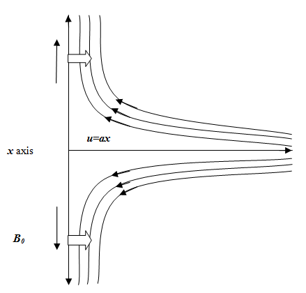
Figure 1. Geometrical illustration
Unsteady type of Eyring-Powell fluid flow on semi-infinite type of porous plate with nonlinear stressing sheet of nanofluids consideration by the influence of radiation absorption and MHD studied. The fluid flow is considered along normal to the plate which is y-direction. Two-dimensional, unsteady fluid flow is stretching by velocity u=ax along x axis where, a>0 indicates the rate of stretching of assumed sheet. At t=0 in starting time, it is considered that T=T∞ and C=C∞ here the particle of fluid is at rest at all points. T∞ and C∞ indicated the fluid temperature and ad joint concentration as well of same fluid far from the layers. We considered a field By=B0 which is uniform type of magnetic field and acted perpendicularly with the fluid. The different parameters physical interruption is represented by the following Figure 1 in co-ordinate system. Under the above assumptions, the governing equations are taken as [24, 32-34],
Equation in terms of continuity
$\frac{\partial u}{\partial x}=-\frac{\partial v}{\partial y}$ (1)
Equation in terms of momentum
$\begin{align} & \frac{\partial u}{\partial t}+u\frac{\partial u}{\partial x}+v\frac{\partial u}{\partial y}=\left( \upsilon +\frac{1}{\rho {{\beta }_{1}}c} \right)\frac{{{\partial }^{2}}u}{\partial {{y}^{2}}} \\ & -\frac{1}{\rho {{\beta }_{1}}{{c}^{3}}}{{\left( \frac{\partial u}{\partial y} \right)}^{2}}\frac{{{\partial }^{2}}u}{\partial {{y}^{2}}}+g\beta (T-{{T}_{\infty }})-\frac{\upsilon }{k}u \\ & +g{{\beta }^{*}}(C-{{C}_{\infty }})-\frac{\sigma B_{0}^{2}}{\rho }u \\ \end{align}$ (2)
Equation in terms of energy
$\begin{align} & \frac{\partial T}{\partial t}+u\frac{\partial T}{\partial x}+v\frac{\partial T}{\partial y}=\frac{\kappa }{\rho \,{{c}_{p}}}\frac{{{\partial }^{2}}T}{\partial {{y}^{2}}}+\frac{\upsilon }{\,{{c}_{p}}}{{\left( \frac{\partial u}{\partial y} \right)}^{2}} \\ & -\frac{1}{\rho \,{{c}_{p}}}\frac{\partial {{q}_{r}}}{\partial y}+\frac{{{Q}_{0}}}{\rho \,{{c}_{p}}}({{T}_{w}}-{{T}_{\infty }}) \\ & +\frac{Q_{1}^{*}}{\rho \,{{c}_{p}}}({{C}_{w}}-{{C}_{\infty }})+\tau \left\{ {{D}_{B}}\left( \frac{\partial T}{\partial y}\frac{\partial C}{\partial y} \right)+\frac{{{D}_{T}}}{{{T}_{\infty }}}{{\left( \frac{\partial T}{\partial y} \right)}^{2}} \right\} \\ \end{align}$ (3)
Concentration equation
$\begin{align} & \frac{\partial C}{\partial t}+u\frac{\partial C}{\partial x}+v\frac{\partial C}{\partial y}={{D}_{B}}\left( \frac{{{\partial }^{2}}C}{\partial {{y}^{2}}} \right)+\frac{{{D}_{T}}}{{{T}_{\infty }}}\frac{{{\partial }^{2}}T}{\partial {{y}^{2}}} \\ & -{{K}_{r}}{{(C-{{C}_{\infty }})}^{P}} \\ \end{align}$ (4)
Considered boundary condition
$\begin{align} & t=0,u={{U}_{0}}=ax,\,v=0,\,T={{T}_{w}},\,\,C={{C}_{w}}\,\,\,\,\text{every}\,\text{where} \\ & t\ge 0,\,u=0,v=0,T={{T}_{\infty }},C={{C}_{\infty }}\,\,\,\,\,\,\,\text{at}\,\,\,\,\,\,x=0 \\ & u=0,T\to {{T}_{\infty }},\,C\to {{C}_{\infty }}\,\,\text{at}\,\,\,\,\,\,y\to \infty \, \\ & u={{U}_{0}}=ax,\,v=0,\,T={{T}_{w}},\,\,C={{C}_{w}}\,\,\,\,\text{at}\,\,\,\,\,\,y=0\, \\ \end{align}$ (5)
Here, u and v indicate velocity parameter, β and β* indicate thermal expansion as well as concentration expansion coefficient, Cw indicates the wall concentration, Tw denotes the wall temperature. In addition, a, b and n are indicating the material constant, kinematic viscosity symbolizes with υ, fluid density indicates by ρ as well as thermal conductivity symbolize by κ. Kc stands for species chemical reaction whereas DB represents Brownian diffusion coefficient also DT is symbolized for thermophoretic diffusion coefficients. The Rosseland approximation in case of radiative type of heat flux is expressed in terms of ${{q}_{r}}=-\left( {4{{\sigma }_{s}}}/{3{{k}_{e}}}\; \right)\left( {\partial {{T}^{4}}}/{\partial y}\; \right) $. Hence, σs indicate the Stefan-Boltzmann term as constant also ke is the average coefficient in the absorption types. In case of minimal temperature difference qr become linear in consider with Taylor series expansion on T4 on T∞. We found, ${{T}^{4}}\approx 4T_{\infty }^{3}T-3T_{\infty }^{4}$ by eliminate higher order terms.
After that the equation in terms of energy (3) found,
$\begin{align} & \frac{\partial T}{\partial t}+u\frac{\partial T}{\partial x}+v\frac{\partial T}{\partial y}=\frac{\kappa }{\rho \,{{c}_{p}}}\frac{{{\partial }^{2}}T}{\partial {{y}^{2}}}+\frac{\upsilon }{\,{{c}_{p}}}{{\left( \frac{\partial u}{\partial y} \right)}^{2}} \\ & +\frac{16{{\sigma }_{s}}T_{\infty }^{3}}{3{{k}_{e}}\rho \,{{c}_{p}}}\frac{{{\partial }^{2}}T}{\partial {{y}^{2}}}+\frac{{{Q}_{0}}}{\rho \,{{c}_{p}}}({{T}_{w}}-{{T}_{\infty }}) \\ & +\frac{Q_{1}^{*}}{\rho \,{{c}_{p}}}({{C}_{w}}-{{C}_{\infty }})+\tau \left\{ {{D}_{B}}\left( \frac{\partial T}{\partial y}\frac{\partial C}{\partial y} \right)+\frac{{{D}_{T}}}{{{T}_{\infty }}}{{\left( \frac{\partial T}{\partial y} \right)}^{2}} \right\} \\ \end{align}$ (6)
Now, applying the below dimensionless terms:
$X=\frac{x{{U}_{0}}}{\upsilon }\,$, $Y=\frac{y{{U}_{0}}}{\upsilon }$, $U=\frac{u}{{{U}_{0}}}$, $V=\frac{v}{{{U}_{0}}}$, $\,\tau =\frac{tU_{0}^{2}}{\upsilon }$, $\theta =\frac{T-{{T}_{\infty }}}{{{T}_{w}}-{{T}_{\infty }}}$, $\,\phi =\frac{C-{{C}_{\infty }}}{{{C}_{w}}-{{C}_{\infty }}}$.
Using these quantities, the dimensionless form of the fundamental equations is getting as below:
Dimensionless form of continuity equation
$\frac{\partial U}{\partial X}+\frac{\partial V}{\partial Y}=0$ (7)
Dimensionless form momentum equation
$\begin{align} & \frac{\partial U}{\partial \tau }+U\frac{\partial U}{\partial X}+V\frac{\partial U}{\partial Y}=\frac{{{\partial }^{2}}U}{\partial {{Y}^{2}}}\left[ 1+\lambda -\lambda \varepsilon {{(\frac{\partial U}{\partial Y})}^{2}} \right] \\ & +{{G}_{r}}\theta +{{G}_{c}}\phi -MU-\frac{U}{{{D}_{a}}} \\ \end{align}$ (8)
Energy equation in term of dimensionless
$\begin{align} & \frac{\partial \theta }{\partial \tau }+U\frac{\partial \theta }{\partial X}+V\frac{\partial \theta }{\partial Y}=\frac{1}{{{P}_{r}}}\left( 1+\frac{16R}{3} \right)\frac{{{\partial }^{2}}\theta }{\partial {{Y}^{2}}}+Q\theta \\ & +{{Q}_{1}}\phi +{{N}_{t}}{{\left( \frac{\partial \theta }{\partial Y} \right)}^{2}}+{{N}_{b}}\frac{\partial \theta }{\partial Y}\frac{\partial \phi }{\partial Y}+{{E}_{c}}{{\left( \frac{\partial U}{\partial Y} \right)}^{2}} \\ \end{align}$ (9)
Concentration equation in term dimensionless
$\frac{\partial \phi }{\partial \tau }+U\frac{\partial \phi }{\partial X}+V\frac{\partial \phi }{\partial Y}=\frac{1}{{{L}_{e}}}\left( \frac{{{\partial }^{2}}\phi }{\partial {{Y}^{2}}}+\frac{{{N}_{t}}}{{{N}_{b}}}\frac{{{\partial }^{2}}\theta }{\partial {{Y}^{2}}} \right)-{{K}_{c}}{{\phi }^{P}}$ (10)
Here with,
$\begin{align} & U=1,\,\,\,\theta =1,\,\,\varphi =1\,\,\,\,\,at\,\,\,\,\,\,y=0 \\ & U=0,\,\,\theta =0,\,\varphi =0\,\,\,\,\,at\,\,\,\,\,\,y\to \infty \, \\ \end{align}$
Hence, the defined physical profiles are formed as below:
Magnetic terms, $M=\frac{{{\sigma }^{'}}B_{0}^{2}\upsilon }{\rho U_{0}^{2}}$, Grash of number, ${{G}_{r}}=\frac{g\beta ({{T}_{w}}-{{T}_{\infty }})\upsilon }{U_{0}^{3}}$, Grash of number in terms of mass, ${{G}_{c}}=\frac{g{{\beta }^{*}}({{C}_{w}}-{{C}_{\infty }})\upsilon }{U_{0}^{3}}$, Darcy number, ${{D}_{a}}=\frac{K'U_{0}^{2}}{{{\upsilon }^{2}}}$, Prandtl number, ${{P}_{r}}=\frac{\rho \,{{c}_{p}}\upsilon }{\kappa }$, radiation parameter, $R=\frac{\sigma T_{\infty }^{3}}{{{k}_{e}}\kappa }$, heat source,$Q=\frac{{{Q}_{0}}\upsilon }{U_{0}^{2}\rho \,{{c}_{p}}}$, heat absorption, ${{Q}_{1}}=\frac{Q_{1}^{*}\upsilon }{U_{0}^{2}\rho \,{{c}_{p}}}\left( \frac{{{C}_{w}}-{{C}_{\infty }}}{{{T}_{w}}-{{T}_{\infty }}} \right) $, Eckert number, ${{E}_{c}}=\frac{U_{0}^{2}}{{{c}_{p}}({{T}_{w}}-{{T}_{\infty }})}$, Lewis number, ${{L}_{e}}=\frac{\upsilon }{{{D}_{B}}}$, Eyring-Powell fluid parameter, $\lambda =\frac{1}{\mu {{B}_{1}}c}$ and $\varepsilon =\frac{U_{0}^{4}}{2{{C}^{2}}{{\nu }^{2}}}$ Brownian parameter,${{N}_{b}}=\frac{\Gamma {{D}_{B}}({{C}_{w}}-{{C}_{\infty }})}{\upsilon }$, thermophoresis parameter${{N}_{t}}=\frac{\Gamma {{D}_{T}}}{{{T}_{\infty }}\upsilon }({{T}_{w}}-{{T}_{\infty }})$, chemical reaction, ${{K}_{c}}=\frac{\upsilon {{K}_{c}}{{({{C}_{w}}-{{C}_{\infty }})}^{p-1}}}{U_{0}^{2}}$ and the chemical reaction power indicate by p.
$\psi$ is the stream function which solves equation (6) in term of continuity (6) and it is along with the velocity parameter in the regular term as,
$U=\frac{\partial \psi }{\partial Y},V=-\frac{\partial \psi }{\partial X}$.
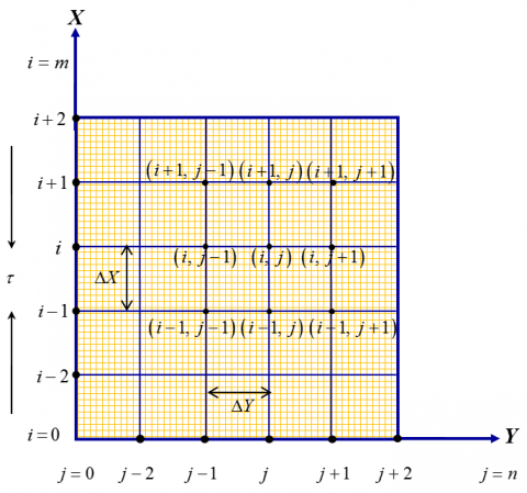
The MHD flow is separated into the two parallel lines along with X, Y, which is set perpendicular to the stretching sheet lines. The Eqns. (7)-(10) are resolved with the help of explicit finite difference procedure. This is why the region of boundary surface is partitioned by some normal lines parallel to X and Y-axes (Figure 2). This is considered as the maximum height of the outer surface layer Ymax= 25 as associated to Y→∞. i.e. Y varies initially 0 to 25 as well as the grid spacing in terms of number in along X and Y axes lines are m= 100, n= 200 respectively by using time Δτ= 0.0005 in step by step.
Equation in terms of continuity
$\frac{{{U}_{i,j}}-{{U}_{i-1,j}}}{\Delta X}=-\frac{{{V}_{i,j}}-{{V}_{i,j-1}}}{\Delta Y}$ (11)
Equation in ters of momentum
$\frac{{{U}_{i,j}}-{{U}_{i-1,j}}}{\Delta X}=-\frac{{{V}_{i,j}}-{{V}_{i,j-1}}}{\Delta Y}\frac{U_{i,j}^{'}-{{U}_{i,j}}}{\Delta \tau }$
$\begin{align} & +{{U}_{i,j}}\frac{{{U}_{i,j}}-{{U}_{i-1,j}}}{\Delta X}+{{V}_{i,j}}\frac{{{U}_{i,j+1}}-{{U}_{i,j}}}{\Delta Y} \\ & =\frac{{{U}_{i,j+1}}-2{{U}_{i,j}}+{{U}_{i,j-1}}}{{{(\Delta Y)}^{2}}}\left\{ 1+\lambda -\lambda \varepsilon {{\left( \frac{{{U}_{i,j+1}}-{{U}_{i,j}}}{\Delta Y} \right)}^{2}} \right\} \\ & -(M+\frac{1}{{{D}_{a}}}){{U}_{i,j}}+{{G}_{r}}{{\theta }_{i,j}}+{{G}_{c}}{{\phi }_{i,j}}\, \\ \end{align}$ (12)
Figure 2. Finite difference grid space
Equation in terms of energy
$\begin{align} & \frac{\theta _{i,j}^{'}-{{\theta }_{i,j}}}{\Delta \tau }+{{U}_{i,j}}\frac{{{\theta }_{i,j}}-{{\theta }_{i-1,j}}}{\Delta X} \\ & +{{V}_{i,j}}\frac{{{\theta }_{i,j+1}}-{{\theta }_{i,j}}}{\Delta Y} \\ & =\frac{1}{{{P}_{r}}}(1+\frac{16}{3}R)\frac{{{\theta }_{i,j+1}}-2{{\theta }_{i,j}}+{{\theta }_{i,j-1}}}{{{(\Delta Y)}^{2}}} \\ & +Q{{\theta }_{i,j}}+{{Q}_{1}}{{\phi }_{i,j}}+{{E}_{c}}{{\left( \frac{{{U}_{i,j+1}}-{{U}_{i,j}}}{\Delta Y} \right)}^{2}} \\ & +{{N}_{b}}\left( \frac{{{\theta }_{i,j+1}}-{{\theta }_{i,j}}}{\Delta Y}.\frac{{{\varphi }_{i,j+1}}-{{\varphi }_{i,j}}}{\Delta Y} \right) \\ & +{{N}_{t}}\left\{ {{\left( \frac{{{\theta }_{i,j+1}}-{{\theta }_{i,j}}}{\Delta Y} \right)}^{2}} \right\} \\ \end{align}$ (13)
Equation in terms of concentration
$\frac{\phi_{i, j}^{\prime}-\phi_{i, j}}{\Delta \tau}+U_{i, j} \frac{\phi_{i, j}-\phi_{i-1, j}}{\Delta X}+V_{i, j} \frac{\phi_{i, j+1}-\phi_{i, j}}{\Delta Y}$
$=\frac{1}{L_{e}}\left\{\begin{array}{l}\left(\frac{\phi_{i, j+1}-2 \phi_{i, j}+\phi_{i, j-1}}{(\Delta Y)^{2}}\right)+ \\ \left(\frac{N_{t}}{N_{b}}\right)\left(\frac{\theta_{i, j+1}-2 \theta_{i, j}+\theta_{i, j-1}}{(\Delta Y)^{2}}\right)\end{array}\right\}-K_{c}\left(\phi_{i, j}\right)^{P}$ (14)
The finite difference technique written in terms of apply below boundary and initial condition,
$U_{i,0}^{n}=R,\,{{\left( \,\theta _{i,0}^{n} \right)}^{'}}=-{{h}_{c}}(1-\theta _{i,0}^{n})=1,\,\,\phi _{i,0}^{n}=1$
$U_{i,L}^{n}=0,\,\,\theta _{i,L}^{n}=0,\,\,\phi _{i,L}^{n}=0$, where, $L\to \infty $.
Here, i and j indicate the grid points along with coordinates X as well as Y, therefore τ=nΔτ, n=1,2,3,4, ..., indicate the time value on that design.
The running investigation demands a stability as well as convergence explanation, the reason behind this is an explicit scheme is being applied. In this study, Eq. (10) will be excluded because Δτ is not evident there. For U, θ and φ, Fourier expansion is being used and the following structure is got at time duration τ also then a time step as,
$\left. \begin{matrix} U:L\left( \tau \right)\,{{e}^{i\alpha X}}{{e}^{i\beta Y}},\,\,\theta :M\left( \tau \right)\,{{e}^{i\alpha X}}{{e}^{i\beta Y}},\,\,\phi :N\left( \tau \right)\,{{e}^{i\alpha X}}{{e}^{i\beta Y}} \\ U:{L}'\left( \tau \right)\,{{e}^{i\alpha X}}{{e}^{i\beta Y}},\,\,\theta :{M}'\left( \tau \right)\,{{e}^{i\alpha X}}{{e}^{i\beta Y}},\,\,\phi :{N}'\left( \tau \right)\,{{e}^{i\alpha X}}{{e}^{i\beta Y}} \\ \end{matrix} \right\}$ (15)
Here, U and V are assumed as constants. Then imposing Eq. (15) into Eqns. (12) to (14) and after simplification the terms become,
$\begin{align} & {L}'={{A}_{1}}L+{{A}_{2}}M+{{A}_{3}}N \\ & {M}'={{A}_{4}}L+{{A}_{5}}M+{{A}_{6}}N \\ & {N}'={{A}_{7}}N+{{A}_{8}}M \\ \end{align}$ (16)
where,
$\begin{align} & {{A}_{1}}=1+\frac{2\Delta \tau }{{{\left( \Delta Y \right)}^{2}}}\left( \cos \beta \Delta Y-1 \right)\left\{ \left( 1+\lambda -\lambda \in \right){{\left( \frac{U}{\Delta Y} \right)}^{2}} \right\}\Delta \tau \\ & -\left( M+\frac{1}{{{D}_{a}}} \right)\Delta \tau -U\frac{\Delta \tau }{\Delta X}\left( 1-{{e}^{-i\alpha \Delta X}} \right)-V\frac{\Delta \tau }{\Delta Y}\left( {{e}^{i\beta \Delta Y}}-1 \right) \\ \end{align}$
$\begin{align} & {{A}_{2}}=\Delta \tau \,{{G}_{r}},\,{{A}_{3}}=\Delta \tau \,{{G}_{c}},\, \\ & {{A}_{4}}=1+\frac{1}{{{P}_{r}}}\left( 1+\frac{16}{3}R \right)\frac{2\Delta \tau }{{{\left( \Delta Y \right)}^{2}}}\left( \cos \beta \Delta Y-1 \right) \\ & +{{N}_{b}}\,\,\phi \frac{\Delta \tau }{{{\left( \Delta Y \right)}^{2}}}{{\left( {{e}^{i\beta \Delta Y}}-1 \right)}^{2}}+{{N}_{t}}\,\,\theta \frac{\Delta \tau }{{{\left( \Delta Y \right)}^{2}}}{{\left( {{e}^{i\beta \Delta Y}}-1 \right)}^{2}} \\ & +Q\Delta \tau -\,U\frac{\Delta \tau }{\Delta X}\left( 1-{{e}^{-i\alpha \Delta X}} \right)-V\frac{\Delta \tau }{\Delta Y}\left( {{e}^{i\beta \Delta Y}}-1 \right),\, \\ & {{A}_{5}}={{E}_{c}}\,U\frac{\Delta \tau }{{{\left( \Delta Y \right)}^{2}}}{{\left( {{e}^{i\beta \Delta Y}}-1 \right)}^{2}},\, \\ & {{A}_{6}}={{Q}_{1}}\Delta \tau ,\,{{A}_{7}}=1+\left( \frac{1}{{{L}_{e}}} \right)\frac{2\Delta \tau }{{{\left( \Delta Y \right)}^{2}}}\left( \cos \beta \Delta Y-1 \right) \\ & -\,U\frac{\Delta \tau }{\Delta X}\left( 1-{{e}^{-i\alpha \Delta X}} \right)-V\frac{\Delta \tau }{\Delta Y}\left( {{e}^{i\beta \Delta Y}}-1 \right)-\,\Delta \tau \,{{K}_{c}}{{\left( \phi \right)}^{p-1}},\, \\ & {{A}_{8}}=\left( \frac{{{N}_{t}}}{{{N}_{b}}\,\,{{L}_{e}}} \right)\frac{2\Delta \tau }{{{\left( \Delta Y \right)}^{2}}}\left( \cos \beta \Delta Y-1 \right). \\ \end{align}$
Now, Eq. (16) can be presented as,
$\left[ \begin{matrix} {{L}'} \\ {{M}'} \\ {{N}'} \\ \end{matrix} \right]=\left[ \begin{matrix} {{A}_{1}} & {{A}_{2}} & {{A}_{3}} \\ {{A}_{5}} & {{A}_{4}} & {{A}_{6}} \\ 0 & {{A}_{8}} & {{A}_{7}} \\ \end{matrix} \right]\left[ \begin{matrix} L \\ M \\ N \\ \end{matrix} \right]$
$\begin{align} & \therefore {\eta }'={T}'\eta \,\,\text{where},\, \\ & {\eta }'=\left[ \begin{matrix} {{L}'} \\ {{M}'} \\ {{N}'} \\ \end{matrix} \right],\,{T}'=\left[ \begin{matrix} {{A}_{1}} & {{A}_{2}} & {{A}_{3}} \\ {{A}_{5}} & {{A}_{4}} & {{A}_{6}} \\ 0 & {{A}_{8}} & {{A}_{7}} \\ \end{matrix} \right]\,\,\text{and}\,\eta \text{=}\,\left[ \begin{matrix} L \\ M \\ N \\ \end{matrix} \right]. \\ \end{align}$
Let us consider, Δτ→0 thus we have, A2→0, A3→0, A5→0, A6→0A8→0.
${T}'=\left[ \begin{matrix} {{A}_{1}} & 0 & 0 \\ 0 & {{A}_{4}} & o \\ 0 & 0 & {{A}_{7}} \\ \end{matrix} \right]$.
Thus, Eigenvalues are got in terms of, λ1 = A1, λ2= A4 and λ3= A7 which solves the following criterion,
$\left| {{A}_{1}} \right|\le 1,\left| {{A}_{4}} \right|\le 1,\left| {{A}_{7}} \right|\le 1$ (17)
Assuming,
${{a}_{1}}=\Delta \tau ,\,{{b}_{1}}=U\frac{\Delta \tau }{\Delta X},{{c}_{1}}=\left| -V \right|\frac{\Delta \tau }{\Delta X},{{d}_{1}}=2\frac{\Delta \tau }{{{\left( \Delta Y \right)}^{2}}}\,$ (18)
where, a1=b1=c1=d1=realnon-negetivenumber, αΔX=mπ, βΔY=nπ, U=+ and V=-.
Then, using Eqns. (17) and (18) together with assuming the highest negative number A1=A4=A5=-1, the stability conditions are achieved after simplification as,
$\begin{align} & \frac{1}{{{P}_{r}}}\left( 1+\frac{16}{3}R \right)\frac{2\Delta \tau }{{{\left( \Delta Y \right)}^{2}}}-2{{N}_{t}}\,\theta \frac{\Delta \tau }{{{\left( \Delta Y \right)}^{2}}} \\ & -2{{N}_{b}}\phi \frac{\Delta \tau }{{{\left( \Delta Y \right)}^{2}}}-\frac{Q\Delta \tau }{2}+U\frac{\Delta \tau }{\Delta X}+\left| -V \right|\frac{\Delta \tau }{\Delta Y}\le 1\,, \\ & \left( \frac{1}{Le} \right)\frac{2\Delta \tau }{{{\left( \Delta Y \right)}^{2}}}+U\frac{\Delta \tau }{\Delta X}+\left| -V \right|\frac{\Delta \tau }{\Delta Y}+\frac{\Delta \tau \,Kr{{\left( \phi \right)}^{p-1}}}{2}\le 1. \\ \end{align}$
By employing at first time U=V=θ=φ=0 at time τ=0 and Δτ=0.0005 for, ΔX=0.20, ΔY=0.25, the current work is examining converging due toPr≥0.058 as well asLe≥0.016.
An Eyring-Powell type fluid flow is being simulated in this work with chemical reaction impact of non-linear order. Explicit scheme is being imposed with the help of a well-known program, namely FORTRAN 6.6.a for solving the basic equations. The simulated results are depicted graphically on different flow region. Meanwhile, the developed visualization of fluid flows is also presented by streamlines as well as isotherms. Moreover, the fluid flows become steady at time τ=30. At this time, the validation of the ongoing investigation is done with Khan et al. [9]. Finally, an excellent agreement is noticed (see Table 1. And Table 2). In Table 1, it is seen that Nusselt number profiles are diminishing for larger values of thermophoresis (Nt) and Brownian (Nb) parameters. It is also can be observed the numerical values obtained in this work are quite similar to the previous work published by Khan et al. [9]. Moreover, in Table 2 it is observed that, the large values of Nt, Nb accelerate the temperature (θ) fields whereas Pr helps to diminish the same field. However, increasing values of M also declines the velocity (U) field. All of the works that is mentioned in Table 2 have given similar outcomes on the discussed fields for these parameters.
Table 1. Comparison of Nusselt number, Nu when, Le=Pr=10; λ=ε=Gr=Gc=M=Da=Q=Q1=Ec=R=Kc=0
|
Parameters |
Khan et al. [9] |
Present result |
|
Nt=Nb= |
Nu |
Nu |
|
0.1 |
0.9541 |
0.9571 |
|
0.2 |
0.3667 |
0.3657 |
|
0.3 |
0.1359 |
0.1363 |
|
0.4 |
0.0499 |
0.0479 |
Table 2. Graphical comparisons with previous results
|
Factor |
Khan et al. [17] |
Malik et al. [2] |
Present result |
|||
|
|
U |
θ |
U |
θ |
U |
θ |
|
M |
|
|
Dec |
|
Dec |
|
|
Nb |
|
Inc |
|
Inc |
|
Inc |
|
Nt |
|
Inc |
|
Inc |
|
Inc |
|
Pr |
|
Dec |
|
Dec |
|
Dec |
Dec - Decrease; Inc - Increase
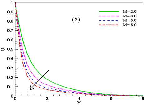
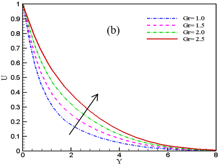
Figure 3. Impact of (a) magnetic parameter, M and (b) Grashof number, Gr on U
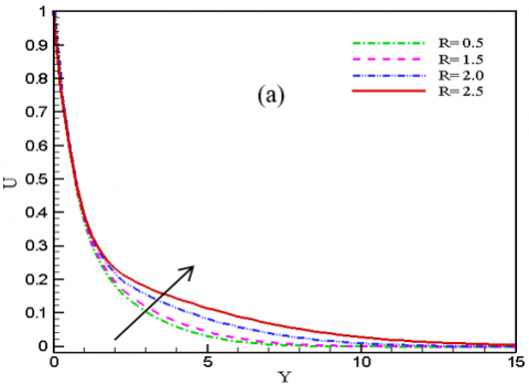
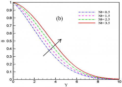
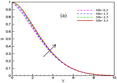
In order to demonstrate the impressions of M indicates magnetic parameter and Grashof number, Gr on velocity fields, Figures 3 (a) and 3 (b) are being exhibited. From these figures, it is found that velocity fields are decelerating 5.98%, 3.13% and1.867% at Y=2 as magnetic parameter rises from 2.0 to 8.0 respectively. Physically, if the high value of magnetic field develops then an opposing force (Lorentz force) starts to down warded the fluid flows in the velocity fields. On the other hand, it is seen that the momentum boundary layers are developing 7.08%, 7.09% and 7.12% respectively as Grashof number, Gr increases from 1.0 to 2.5 (Figure 3 (b)). Because, larger Grashof number increases the thermal buoyancy force, which accelerates the fluid motion in the velocity profiles. On the velocity as well as temperature fields, the impacts of radiation parameter, R and thermophoresis, Nt are being illustrated respectively (Figures 4 (a) and 4(b)). It is observed that both fields are developing for increasing data of radiation and thermophoresis parameters. Here the rate of increased 1.29%, 3.92%, 2.99% from initial value to final at Y=5 for thermal radiation and in case of thermophoresis the increased rate in percentage 4.69%, 5.41%, 6.03% at Y=4. Here, radiation parameter aids to increase the heat flux divergence, which increases the respective fluid field. Again, the uncontrolled motion of fluid particles helps to accelerate the respective fields. However, the same phenomenon can be observed for Brownian parameter, Nb, on temperature field (Figure 5 (a)) where the upward magnitude in percentage is 1.61%, 1.55%, 1.46% at Y=2.
Figure 4. Impact of (a) radiative parameter, R on U and (b) thermophoresis, Nt on θ
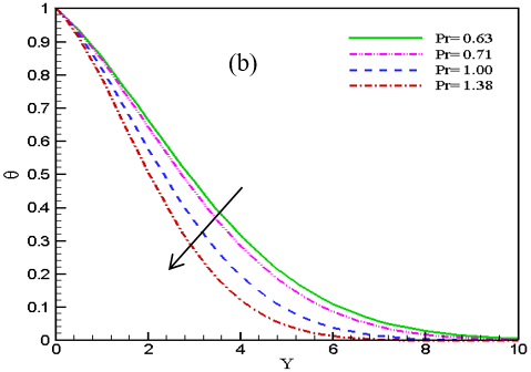
Here, it can be seen that the thermophoresis parameter is affecting the temperature field significantly rather than the Brownian motion parameter. Because larger data of thermophoresis increases the heat capacity of fluid particles, it eventually accelerates the particles' motion. On the other hand, small data of Nb represents particles with less motion [20, 25]. Due to this fact, these particles collide with less motion which finally accelerates the temperature filed but it is not that much significant like thermophoresis parameters. The impression of Prandtl number, where this is symbolized Pr on temperature profiles are examined in Figure 5 (b). It can be perceived that for improving Pr the temperature profiles decline 2.136%, 6.698% and 7.036% at Y=2 as it varies from 0.63 to 1.38 respectively. It is known that Prandtl number tells us how fast thermal diffusion takes place in comparison to momentum diffusion. Usually, Prandtl number defines that the thermal boundary layer is large if Pr<<1 and it is small when Pr>>1. Also the definition (Pr=ʋ/α=ʋρcp/κ) tells us that Prandtl number is inversely proportional to thermal diffusivity. This physical phenomenon is displayed in Figure 5 (b).
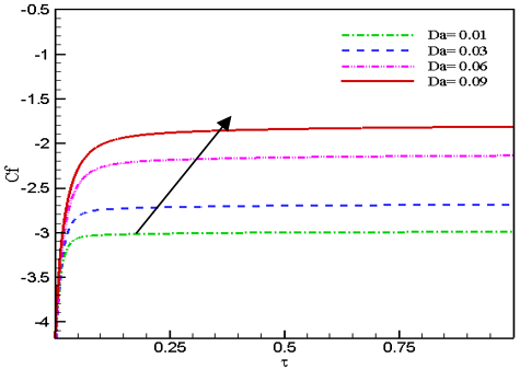
Figure 6 is plotted to demonstrate the impressions of Darcy number, Da on skin friction profiles. Darcy number is exhibiting accelerating behavior on skin friction fields as it changes from 0.01 to 0.09. Hence, numerical value of Darcy number with respect to skin friction displayed in Table 3 at Y=0.5 where the incremented pattern is observed vividly.
Figure 5. Impact of (a) Brownian parameter, Nb and (b) Prandtl number, Pr on θ
Figure 6. Impact of Darcy number, Da on Cf
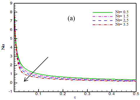
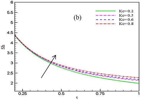
From the plotting of Nusselt number, Nu (Figure 7 (a))and Sherwood number, Sh (Figure 7 (b)) it is understandable that increasing data of thermophoresis, Nt are diminishing the Nu fields in percentage 7.11%, 5.83%, 4.78% at Y=0.5 whilst chemical reaction, Kc raises the curve of Sh by 2.32%, 2.38% and 2.44% as Kc increases from 0.2 to 0.8. Physically, thermophoresis parameter accelerates the motion of the fluid particles and increases the fluid temperature. On the other hand, a destructive chemical reaction (Kc>0) increases the disturbances between the molecules, due to that the motion of the particles get to develop and diffuses quickly at the wall. However, the Nusselt number, as well as Sherwood number in terms of magnitude over thermophoresis parameter and chemical reaction, are presented in Table 3 in bold number for more distinct vision of graphical changed.
Figure 7. Impact of (a) thermophoresis, Nt on Nu and (b) chemical reaction, Kc on Sh
Table 3. The values of wall friction (Cf), heat transfer (Nu) as well as mass transfer (Sh) at the surface for different parameters at τ= 0.5
|
Parameters |
Cf |
Nu |
Sh |
|
Da=0.01 |
-2.99470 |
0.34627 |
2.83014 |
|
Da =0.03 |
-2.70846 |
0.56119 |
3.87599 |
|
Da =0.07 |
-2.15235 |
0.34585 |
2.83038 |
|
Da =0.09 |
-1.84353 |
0.34576 |
2.83042 |
|
Nt=0.50 |
-0.86124 |
0.34577 |
2.83036 |
|
Nt =1.50 |
-0.84456 |
0.27468 |
2.82784 |
|
Nt =2.50 |
-0.83613 |
0.21635 |
2.96399 |
|
Nt =3.50 |
-0.83377 |
0.16855 |
3.17531 |
|
Kc=0.20 |
-0.86023 |
0.34546 |
2.76441 |
|
Kc =0.50 |
-0.86124 |
0.34577 |
2.83036 |
|
Kc =0.60 |
-0.86156 |
0.34587 |
2.85163 |
|
Kc =0.80 |
-0.86221 |
0.34606 |
2.89315 |
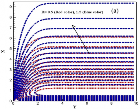
The improved visualization of the fluid flow is being exhibited in Figures 8 (a) and 8 (b), respectively. This sort of work is done on streamlines and isothermal lines. Here, two types of view are presented such that flood view and line view. The influence of radiation parameter, R is showed on streamlines (Figure 8 (a) (line view)) and isothermal lines (Figure 8 (b) (line view)). Interestingly, momentum and thermal boundary layers are developing inside the layer for rising values of R. Because the molecules get heated up then the thickness of momentum and thermal boundary surfaces get developed due to the divergence of heat flux.
Figure 8. (a) Streamlines (line view) and (b) Isotherms (line view) for R =0.5, 1.5
The main focus of this analysis is to explain the characteristics of Eyring-Powell fluid flow on a stretching sheet with the presence of nanoparticles. Explicit finite difference method is used to solve the fundamental equations numerically. The default numerical values for this work are considered as p=3, Gr=1.0, Gm=1.0, M=2.0, Nb=Nt=0.001, Pr=0.71, R=0.5, Q=0.4, Le=5.0, Kc=0.5 and Da=1.0 [24, 25, 32]. Furthermore, it is possible to investigate this work by using different methods such as Rung-Kutta based on the shooting technique, Homotopy analysis method, etc. This research's key findings are: to improve magnetic parameter values, and the velocity field tends to decline whilst increasing data of Grash of number and radiation parameter help develop the momentum boundary layers. Moreover, the temperature profiles enhance the increment in thermophoresis and Brownian parameters, whereas an opposite incident is being noticed for Prandtl number. Also, the concentration field diminishes when the values of the Schmidt number get enhances. Besides this, friction coefficient distribution develops for up surging values of Darcy number. However, the Nusselt number profile goes down for rising thermophoresis parameters and developing values of chemical reaction diminishes mass transfer at the wall surface. Finally, larger data of radiation accelerates the boundary layer thickness in streamlines and isothermal lines.
|
$B_{0}$ |
Magnetic field, [$\mathrm{Wbm}^{-2}$] |
|
C |
Concentration component |
|
$C_{P}$ |
Specific heat, [Jkg-1K-1] |
|
$C_{w}$ |
Wall Concentration, [mol.] |
|
$C_{\infty}$ |
Ambient Concentration |
|
Cf |
Skin friction, [-] |
|
G |
Gravitational acceleration, $\left[\mathrm{ms}^{-2}\right]$ |
|
Gr |
Thermal Grashof number, [-] |
|
Gm |
Mass Grashof number, [-] |
|
Kr |
Chemical reaction parameter, [-] |
|
Le |
Lewis number, [-] |
|
M |
Magnetic parameter, [-] |
|
Nb |
Brownian parameter, [-] |
|
Nt |
Thermophoretic parameter, [-] |
|
Nu |
Nusselt number, [-] |
|
Pr |
Prandlt number, [-] |
|
qr |
Heat radiative flux, $\left[\mathrm{kgm}^{-2}\right]$ |
|
Ra |
Radiation parameter, [-] |
|
Sh |
Sherwood number, [-] |
|
T |
Temperature, [K] |
|
$T_{\infty}$ |
Ambient temperature |
|
$T_{w}$ |
Surface temperature |
|
$u_{0}$ |
Uniform velocity, $\left[\mathrm{ms}^{-1}\right]$ |
|
u, v |
Dimensional velocity of the fluid in x and y direction |
|
U |
Non-dimensional velocity, [-] |
|
$\theta$ |
Non-dimensional temperature, [-] |
|
$\phi$ |
Dimensionless concentration, [-] |
|
Greek symbols |
|
|
$v$ |
Kinematic viscosity, $\left[m^{2} s^{-1}\right]$ |
|
τ |
Dimensionless time |
|
$K$ |
Thermal conductivity,$\left[W m^{-1} K^{-1}\right]$ |
|
$\sigma_{s}$ |
Stefan-Boltzmann constant, $\left[W m^{2} K^{-4}\right]$ |
|
ρ |
Density, [kgm-3] |
|
$\Gamma$ |
Rate time constant, [s] |
|
$\lambda$ |
Eyring-Powell fluid parameter |
[1] Powell, R.E., Eyring, H. (1944). Mechanism for the relaxation theory of viscosity. Nature, 154: 427-428.
[2] Malik, M.Y., Khan, I., Hussain, A., Salahuddin, T. (2015). Mixed convection flow of MHD Eyring-Powell nanofluid over a stretching sheet: A numerical study. AIP Advances, 5117118. https://doi.org/10.1063/1.4935639
[3] Bachok, N., Ishak, A., Pop, I. (2012). Unsteady boundary-layer flow and heat transfer of a nanofluid over a permeable stretching/shrinking sheet. International Journal of Heat and Mass Transfer, 55: 2102-2109. https://doi.org/10.1016/j.ijheatmasstransfer.2011.12.013
[4] Naseem, F., Shafiq, A., Zhao, L., Naseem, A. (2017). MHD bio convective flow of Powell Eyring nanofluid over stretched surface. AIP Advances, 7: 065013. https://doi.org/10.1063/1.4983014
[5] Rosca, A.V., Pop, I. (2014). Flow and heat transfer of Powell-Eyring fluid over a shrinking surface in a parallel free stream. International Journal of Heat and Mass Transfer, 71: 321-327. http://dx.doi.org/10.1016/j.ijheatmasstransfer.2013.12.020
[6] Banerjee, A., Zaib, A., Bhattacharyyan, K., Mahato, S.K. (2018). MHD mixed convection flow of a non-Newtonian Powell-Eyring fluid over a permeable exponentially shrinking sheet. Frontiers in Heat and Mass Transfer, 10: 30. http://dx.doi.org/10.5098/hmt.10.30
[7] Ramzan, M., Bilal, M., Kanwal, S., Chung, J.D. (2017). Effects of variable thermal conductivity and non-linear thermal radiation past an Eyring Powell nanofluid flow with chemical reaction. Communication in Theoretical Physics, 67: 723-731. http://dx.doi.org/10.1088/0253-6102/67/6/723
[8] Khan, I., Malik, M.Y., Salahuddin, T., Khan, M., Rehman, K.U. (2017). Homogenous-heterogeneous reactions in MHD flow of Powell-Eyring fluid over a stretching sheet with Newtonian heating. Neural Computer and Application, 30: 3581-3588. http://dx.doi.org/10.1007/s00521-017-2943-6
[9] Khan, N.A., Sultan, F., Khan, N.A. (2015). Heat and mass transfer of thermophoretic MHD flow of Powell-Eyring fluid over a vertical stretching sheet in the presence of chemical reaction and joule heating. International Journal Chemical Reactor Engineering, 13: 37-49. https://doi.org/10.1515/ijcre-2014-0090
[10] Ara, A., Khan, N.A., Khan, H., Sultan, F. (2014) Radiation effect on boundary layer flow of an Eyring-Powell fluid over an exponentially shrinking sheet. Ain Shams Engineering Journal, 5: 1337-1342. https://doi.org/10.1016/j.asej.2014.06.002
[11] Malik, M.Y., Hussain, A., Nadeem, S. (2013). Boundary layer flow of an Eyring-Powell model fluid due to a stretching cylinder with variable viscosity. Scientia Iranica B, 20: 313-321. https://doi.org/10.1016/j.scient.2013.02.028
[12] Rahimi, J., Ganji, D.D., Khaki, M., Hosseinzadeh, K. (2017). Solution of the boundary layer flow of an Eyring-Powell non-Newtonian fluid over a linear stretching sheet by collocation method. Alexandria Engineering Journal, 56: 621-627. https://doi.org/10.1016/j.aej.2016.11.006
[13] Mahanthesh, B., Gireesha, B.J., Gorla, R.S.R. (2017). Unsteady three-dimensional MHD flow of a nano Eyring-Powell fluid past a convectively heated stretching sheet in the presence of thermal radiation, viscous dissipation and Joule heating. Journal of the Association of Arab Universities for Basic and Applied Sciences, 23: 75-84. https://doi.org/10.1016/j.jaubas.2016.05.004
[14] Khader, M.M., Megahed, A.M. (2016). Numerical treatment for flow and heat transfer of Powell-Eyring fluid over an exponential stretching sheet with variable thermal conductivity. Meccanica, 51: 1763-1770. https://doi.org/10.1007/s11012-015-0336-4
[15] Javed, T., Ali, N., Abbas, Z., Sajid, M. (2013). Flow of an Eyring-Powell non Newtonian fluid over a stretching sheet. Chemical Engineering Communications, 200: 327-336. http://dx.doi.org/10.1080/00986445.2012.703151
[16] Akbar, N.S., Ebaid, A., Khan, Z.H. (2015). Numerical analysis of magnetic field effects on Eyring-Powell fluid flow towards a stretching sheet. Journal of Magnetism and Magnetic Materials, 382: 355-358. http://dx.doi.org/10.1016/j.jmmm.2015.01.088
[17] Khan, M.I., Waqas, M., Alsaedi, A., Hayat, T., Khan, M.I. (2017). Theoretical investigation of the doubly stratified flow of an Eyring-Powell nanomaterial via heat generation/absorption. The European Physical Journal Plus, 132: 489. http://dx.doi.org/10.1140/epjp/i2017-11753-8
[18] Babu, M.J., Sandeep, N., Raju, C.S. (2016). Heat and mass transfer in MHD Eyring-Powell nanofluid flow due to cone in porous medium. International Journal of Engineering Research in Africa, 19: 57-74. http://dx.doi.org/10.4028/www.scientific.net/JERA.19.57
[19] Ghadikolaeia, S.S., Hossein Zadehb K., Ganji, D.D. (2017). Analysis of unsteady MHD Eyring-Powell squeezing flow in stretching channel with considering thermal radiation and Joule heating effect using AGM. Case Studies in Thermal Engineering, 10: 579-594. https://doi.org/10.1016/j.csite.2017.11.004
[20] Bég, O.A., Khan, M.S., Karim, I., Alam, M.M., Ferdows, M. (2014). Explicit numerical study of unsteady hydromagnetic mixed convective nanofluid flow from an exponentially stretching sheet in porous media. Applied Nanoscience, 4: 943-957. https://doi.org/10.1007/s13204-013-0275-0
[21] Khan, M.S., Karim, I., Ali, L.E., Islam, A. (2012). Unsteady MHD free convection boundary-layer flow of nanofluid along a stretching sheet with thermal radiation and viscous dissipation effects. International Nano Letters, 2: 1-9. https://doi.org/10.1186/2228-5326-2-24
[22] Arifuzzaman, S.M., Khan, M.S., Hossain, K.E., Islam, M.S., Akter, S., Roy, R. (2017). Chemically reactive viscoelastic fluid flow in presence of nano particle through porous stretching sheet. Frontiers in Heat and Mass Transfer, 9: 5. https://doi.org/10.5098/hmt.9.5
[23] Arifuzzaman, S.M., Mehedi, M.F.U., Al-Mamun, A., Khan, M.S. (2017). Magnetohydrodynamic micropolar fluid flow in presence of nanoparticles through porous plate: A numerical study. International Journal of Heat and Technology, 36: 936-948. https://doi.org/10.18280/ijht.360321
[24] Reza-E-Rabbi, S., Arifuzzaman, S.M., Sarkar, T., Khan, M.S., Ahmmed S.F. (2020). Explicit finite difference analysis of an unsteady MHD flow of a chemically reacting Casson fluid past a stretching sheet with Brownian motion and thermophoresis effects. Journal of King Saud University - Science, 32: 690-701. https://doi.org/10.1016/j.jksus.2018.10.017
[25] Reza-E-Rabbi, S., Ahmmed, S.F., Arifuzzaman, S.M., Sarkar, T., Khan, M.S. (2020). Computational modeling of multiphase fluid flow behavior over a stretching sheet in presence of nanoparticles. Engineering Science and Technology, an International Journal, 23: 605-617. http://dx.doi.org/10.1016/j.jestch.2019.07.006
[26] Arifuzzaman, S.M., Khan, M.S., Al-Mamun, A., Reza-E-Rabbi, S., Biswas, P. (2019). Hydrodynamic stability and heat and mass transfer flow analysis of MHD radiative fourth-grade fluid through porous plate. Journal of King Sauid University- Science, 31: 1388-1398. http://dx.doi.org/10.1016/j.jksus.2018.12.009
[27] Reza-E-Rabbi, S., Arifuzzaman, S.M., Khan, M.S., Sarkar, T., Ahmmed, S.F. (2019). Periodic magnetohydrodynamic simulation of newtonian and non- Newtonian fluids flow behaviour past a stretching sheet with nanoparticles. AIP Conference Proceedings, 2121: 070006. http://dx.doi.org/10.1063/1.5115913
[28] Al-Mamun, A., Arifuzzaman, S.M., Reza-E-Rabbi, S., Biswas, P., Khan, M.S. (2018). Numerical Investigation of boundary-layer flow of Sisko nanofluids through a nonlinear stretching sheet with MHD and thermal radiation effects. International Journal of Heat and Technology, 37(1): 285-295. https://doi.org/10.18280/ijht.370134
[29] Sarker, T, Arifuzzaman, S.M., Reza-E-Rabbi, S., Khan, M.S., Ahmmed, S.F. (2019) Computational modelling of chemically reactive and radiative flow of Casson-Carreau nanofluids over an inclined cylindrical surface with bended Lorentz force presence in porous medium. AIP Conference Proceedings, 2121: 050006. http://dx.doi.org/10.1063/1.5115893
[30] Biswas, P., Arifuzzaman, S.M., Rahman, M.M., Khan, M.S. (2017). Effects of periodic magnetic field on 2D transient optically dense gray nanofluid over a vertical plate: A computational EFDM study with SCA. Journal of Nanofluids, 7: 1-10. https://doi.org/10.1166/jon.2018.1434
[31] Arifuzzaman, S.M., Khan, M.S., Mehedi, M.F.U., Rana, B.M.J., Biswas, P., Ahmed, S.F. (2018). Chemically reactive and naturally convective high speed MHD fluid flow through an oscillatory vertical porous plate with heat and radiation absorption effect. Engineering Science and Technology, 21: 215-228. http://dx.doi.org%2F10.1016%2Fj.jestch.2018.03.004
[32] Narayana, P.V.S., Tarakaramu1, N., Akshit, S.M., Ghori, J.P. (2017). MHD flow and heat transfer of an Eyring-Powell fluid over a linear stretching sheet with viscous dissipation- a numerical study. Frontiers in Heat and Mass Transfer, 9: 9. http://dx.doi.org/ 10.5098/hmt.9.9
[33] Hayat, T., Ali, S., Farooq, M.A., Alsaedi, A. (2015). On comparison of series and numerical solutions for flow of Eyring-Powell fluid with Newtonian heating and internal heat generation/absorption. PLoS One, 10: 9. http://dx.doi.org/10.1371/journal.pone.0129613
[34] Hussain, A., Malik, M.Y., Khan, F. (2013). Flow of an Eyring-Powell model fluid between coaxial cylinders with varable viscosity. Chinese Journal of Engineering, 7: 808342. https://doi.org/10.1155/2013/808342