Rajasekhar Vatambeti | P.K. Dhal*
© 2021 IIETA. This article is published by IIETA and is licensed under the CC BY 4.0 license (http://creativecommons.org/licenses/by/4.0/).
OPEN ACCESS
Congestion management plays an important role in the operation, control, and safety of the grid. This paper proposes the multiverse optimization (MVO) algorithm for the congestion management of the IEEE 30 bus system, aiming to identify line congestion, and eliminate it at the minimum congestion price (i.e., the minimum loss). The continuation power flow (CPF) mechanism is adopted to analyze the voltage stability and maximum load capacity of the grid. The MVO algorithm helps to boost the voltage with a photovoltaic (PV) device, whenever the grid became unstable. The optimal position of the device is found through six iterations, and the fitness function is found capable of maximizing loading parameters, while minimizing power loss. The new approach is evaluated under different operating conditions, namely, in the presence of an MVO-tuned PV grid, and in the absence of a PV grid. The results show that the MVO-tuned PV grid performed much better than the grid without a PV.
photovoltaic (PV), voltage stability, continuation power flow (CPF), multiverse optimization (MVO), IEEE 30 bus, real power, reactive power, load capability
For the safety of the power network, each grid needs to operate within stability limits. The grid might be congested, due to the lack of compatible generators and transmitters. Congestion could be triggered by unexpected events like power outage, sudden increase of load demand, and tool failure. The incidence of congestion in the energy program disturbs the grid, and causes more outages to interconnected systems. Frequent outages pose a serious threat to the power system: the tools will be damaged, and the power quality will be undermined. To cope with the threat, the energy program for the grid must be able to rectify congestion instantly.
The voltage of the congested grid can be stabilized with many compensation devices, or distribution generation (DG) unit. Focusing on bus sensitivity and wind availability, Suganthi et al. [1] discussed how to control congestion in the grid of wind farms: a differential evolution (DE)-based strategy was proposed to reduce transmission line congestion by rescheduling generators and constructing additional wind farms, and an updated mutation operator was introduced to improve the performance of the strategy. Remha et al. [2] examined the ideal location and size of DG units in radial distribution networks, and optimized the two parameters through three latest techniques: injecting active power, injecting reactive power, and injecting both powers. To choose the best site for DG units, Arief and Nappu [3] defined the tangent vector of the continuation power flow (CPF) method as the differential change ratio of voltage to load, and iteratively estimated the DG size in each place until the grid reaches the stable state.
Inspired by cosmological concepts like white hole, blackhole, and wormhole [4], Mirjalili et al. [5] tried to reduce grid voltage by integrating a wind turbine with a squirrel cage induction generator, and adopted the CPF method to locate wind farms and stabilize static voltage. Based on the 24h power demand, Sharma et al. [6] tested the reliability of the hourly load shapes of IEEE-30 and IEEE-57 bus systems, compared the results of flower pollination algorithm (FPA)-DE hybrid optimization with those of DE optimization, and confirmed the excellence of both strategies in congestion reduction. Using a modified IEEE-39 bus New England test system, Gope et al. [7] attempted to minimize congestion cost and enhance system safety through congestion management with and without a pump storage hydro unit (PSHU), and proposed a congestion management method based on bus sensitivity and generator sensitivity; the former was adopted to determine the location of wind farms [8]. Focusing on the optimal power flow (OPF) problem, Hooshmand et al. [9] established an objective function to minimize generator fuel and emission penalty cost, combined the bacterial foraging (BF) algorithm with the Nelder-Mead (NM) approach to solve the OPF problem, and optimized the size and position of thyristor-controlled series capacitor (TCSC) by minimizing the cost of generation, emissions, and the device.
Kashyap and Kansal [10] hybridized the firefly algorithm with DE optimization, and proved that the hybrid approach can efficiently handle congestion in a deregulated market by rescheduling generators, while satisfying both technical and economic constraints. Nappu et al. [11] discussed the concepts, technical challenges, and methods for alternate redispatch mechanism, formulated a locational management price scheme based on an optimization strategy for congestion control. Thangalakshmi and Valsalal [12] suggested that, in a deregulated power system, the independent system operator (ISO) faces the difficult task of managing transmission line congestion, and took account of the economic factors of most congestion management solutions. Verma and Mukherjee [13] put forward a generator rescheduling strategy based on ant lion optimizer (ALO), a novel algorithm inspired by the hunting mechanism of ant lions, to manage grid congestion. The effectiveness of the strategy was verified on modified IEEE 30-bus, modified IEEE 57-bus, and modified IEEE 118-bus, under the security constraints of load bus voltage and line loading impact. The strategy was found to outperform several modern optimization algorithms. Khatavkar et al. [14] improved the branch loading index of the grid by reducing losses, and enhancing voltage stability.
To solve the dynamic direct current (DC) optimal power flow (DDCOPF) problem, Dehnavi and Abdi [15] identified the ideal buses with such indices as power transfer distribution factors (PTDFs), and available transfer capability (ATC), and demonstrated the merits of their identification method: reducing line congestion, increasing benefits of consumers and ISO, improving load curve features, preventing line outages and blackouts, and enhancing grid dependability. For cost-free mitigation of grid congestion, Vijayakumar [16] took flexible alternating current (AC) transmission system (FACTS) as a cost-free method, optimized the positions of TCSC and unified power flow controller (UPFC) to relieve grid congestion, and introduced the genetic algorithm (GA) to solve the complex objective function in congestion management. Reddy and Singh [17] offered two distinct ways to find a suitable position for UPFC: one is based on sensitivity, and the other is based on pricing. The sensitivity-based approach aims to reduce the overall loss of the system. Ravindrakumar and Chandramohan [18] obtained a set of Pareto optimal solutions for grid congestion alleviation by the non-dominated sorting genetic algorithm II (NSGA-II).
This paper handles overload through generator rescheduling, eliminating the need for load shedding, and proposes a new stochastic population-based algorithm called multiverse optimization (MVO). Through the test on an IEEE 30 bus system, our approach was proved suitable under two different congestion scenarios. The remainder of this paper is organized as follows: Section 2 carries out the CPF analysis; Section 3 examines the PV energy storage system; Section 4 introduces the MVO technique; Section 5 analyzes the IEEE 30 bus system; Section 6 connects the system with the PV tuned by MVO; Section 7 summarizes the strengths of MVO in congestion control.
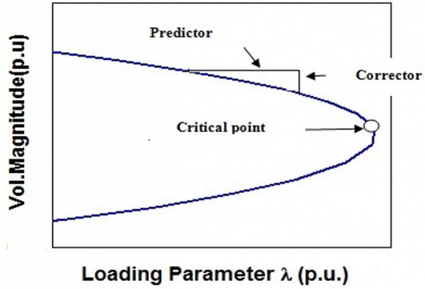
Figure 1. CPF graph
The CPF is a useful tool to determine the voltage stability and maximum load capability of the grid. The maximum load of the grid depends on the critical point, a.k.a. the maximum point. The dependence can be analyzed with predictor and corrector measures. The grid load either fails or reaches the maximum level. If the load surpasses this level, the grid will become unstable (Figure 1). The voltage impact, active power, reactive power, and grid safety are all influenced by the PV grid. This paper investigates the effect of a PV grid on the load capacity and stability in the IEEE 30 node test network.
The PV energy storage system is commonly called the distributed energy storage system. Studies have shown that the PV system is very stable, its proximity to load and decentralized structure. Since the solar radiation sometimes falls below zero, solar power alone cannot address the congestion problem. The energy generated by a PV device can be calculated by:
$S_{G}^{t}=S_{r}\left\{1+\left(T_{r}-T_{a}\right) \propto\right\} \times \frac{i_{r r}^{t}}{1000}$ (1)
Verma and Mukherjee [13] stated that the big bang theory explains the origin of everything in the universe, but the multiverse offers another theory: there are more than one big bang, each of which creates a new universe. There might be different physical laws in these universes. The multiverse theory inspires the MVO algorithm, which has three guiding principles: whitehole, blackhole, and wormhole. No white hole is permitted in the universe by the big bang theory, many blackholes have been observed so far, and a wormhole is a portal connecting two universes. Each universe has a unique inflation rate, which can be used to calculate fitness. The MVO algorithm can be implemented in two steps: exploration and exploitation.
4.1 Procedure of proposed technique
Step 1. Set up the constraints of the MVO and PV generation.
Step 2. Generate a set of random universes through roulette wheel selection.
Step 3. Calculate the inflation rate (fitness) of each universe.
Step 4. Sort the universes by inflation rate.
Step 5. Update the position of each universe.
Step 6. Output the result if the termination condition is satisfied.
Step 7. Otherwise, repeat Steps 2-6.
4.2 Selection of fitness function
Congestion management attempts to reduce power loss under grid constraints, i.e., keeping operating parameters like voltage, reactive power, and angle within their prescribed ranges. The fitness function aims to maximize the loading parameters, that is, bolster the full load capacity. The fitness can be calculated by:
Fitness=maximum loading parameter $(\lambda)+$ minimum active power loss (2)
The active power generated by the PV grid falls between 1 and 10.
4.3 Problem formulation
The research problem has two objectives: optimal location of the proposed system, and optimizing the size of the PV (2.26 MW).
4.3.1 Optimal location of the proposed system
The marginal price of the optimal location for the congestion line should be correctly identified. It is the optimal location of the distributed energy storage system.
Minimize f(x);
Subjected to,
$g_{i}(x) \leq 0 \forall i \in\{1,2,3, \ldots, n\}$ (3)
$h_{i}(x)=0 \forall i \in\{1,2,3, \ldots, n\}$ (4)
The optimal power flow depends on the minimum fuel cost. It’s given as:
Minimize $\sum_{n=1}^{m} f_{n}\left(P_{g}^{n}\right)$ (5)
(a) Power balance constraint
$P_{n}=f_{x}(V, \delta)$ implies to zero (6)
(b) Inequality constraints
$P_{g(\min )}<P_{g}<P_{g(\max )}$ (7)
$Q_{q(\min )}<Q_{g}<Q_{g(\max )}$ (8)
$V_{(\min )}<V<V_{(\max )}$ (9)
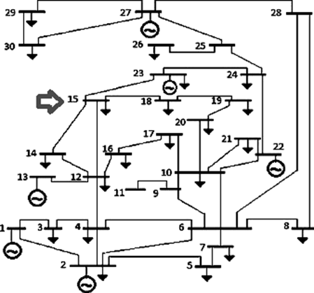
Figure 2. Single line representation of the IEEE 30 node test network
The grid output is evaluated on an IEEE 30 node test network containing 6 generators and 20 loads, as well as a PV network. After continuous iterations, the PV network is placed at node 15 by the proposed algorithm. The grid is considered with and without PV power generation. With the growing load, the grid became congested. To ease the congestion, the PV network is integrated to the grid, enhancing the load capacity. Besides, the size of the PV network tuned by the MVO is optimized to improve the network performance (Figure 2).
5.1 PV analysis on voltage profile, active and reactive powers
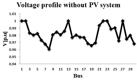
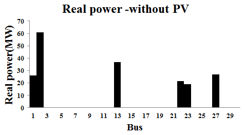
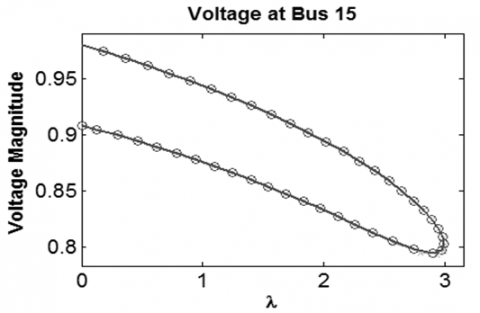
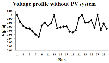
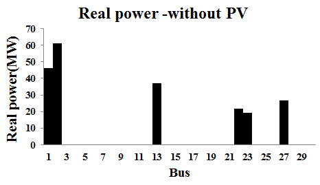
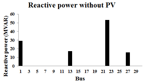
Figure 3 shows the voltage profile of the unit without PV network. In this case, the highest voltage profile is obtained through iterations. The active and reactive power profiles of the unit without PV network are displayed in Figures 4 and 5, respectively. Figure 6 depicts the load capacity curve of the unit. Obviously, the highest load capacity is 2.9859. Table 1 lists the parameters of the unit without PV network. Table 2 shows the total generation and losses.
Figure 3. Voltage profile of the unit without PV network
Figure 4. Active power profile of the unit without PV network
Figure 5. Reactive power profile of the unit without PV network
Figure 6. Load capacity curve of the unit without PV network
Table 1. Parameters of the unit without PV network
|
Bus No |
Volt in p.u |
P in p.u |
Q in p.u |
|
1 |
1.00000 |
25.97380 |
-0.9984 |
|
2 |
1.00000 |
60.97000 |
31.9989 |
|
3 |
0.98314 |
0.00000 |
0.00000 |
|
4 |
0.98009 |
0.00000 |
0.00000 |
|
5 |
0.98241 |
0.00000 |
0.00000 |
|
6 |
0.97318 |
0.00000 |
0.00000 |
|
7 |
0.96736 |
0.00000 |
0.00000 |
|
8 |
0.96062 |
0.00000 |
0.00000 |
|
9 |
0.98051 |
0.00000 |
0.00000 |
|
10 |
0.98440 |
0.00000 |
0.00000 |
|
11 |
0.98051 |
0.00000 |
0.00000 |
|
12 |
0.98547 |
0.00000 |
0.00000 |
|
13 |
1.00000 |
37.00000 |
11.3528 |
|
14 |
0.97668 |
0.00000 |
0.00000 |
|
15 |
0.98023 |
0.00000 |
0.00000 |
|
16 |
0.97740 |
0.00000 |
0.00000 |
|
17 |
0.97687 |
0.00000 |
0.00000 |
|
18 |
0.96844 |
0.00000 |
0.00000 |
|
19 |
0.96529 |
0.00000 |
0.00000 |
|
20 |
0.96917 |
0.00000 |
0.00000 |
|
21 |
0.99338 |
0.00000 |
0.00000 |
|
22 |
1.00000 |
21.59000 |
39.5699 |
|
23 |
1.00000 |
19.20000 |
7.95095 |
|
24 |
0.98857 |
0.00000 |
0.00000 |
|
25 |
0.99021 |
0.00000 |
0.00000 |
|
26 |
0.97219 |
0.00000 |
0.00000 |
|
27 |
1.00000 |
26.9100 |
10.5405 |
|
28 |
0.97471 |
0.00000 |
0.00000 |
|
29 |
0.97960 |
0.00000 |
0.00000 |
|
30 |
0.96788 |
0.00000 |
0.00000 |
Table 2. Total generation and losses of the unit without PV network
|
|
Generation |
Load |
Losses |
|
Watt power (MW) |
191.64 |
189.20 |
2.44 |
|
Wattles power (MVAR) |
100.41 |
107.20 |
6.79 |
5.2 10% and 20% rises in load without PV system
Figure 7 shows the voltage profile of the unit without PV network with a load increase of 10%. In this case, the voltage peaked at 1. The active and reactive power profiles of the unit without PV network are displayed in Figures 8 and 9, respectively. Figure 10 depicts the load capacity curve of the unit. In this case, the highest load capacity is 1.8254. Table 3 lists the parameters of the unit without PV network with a load increase of 10%. Table 4 shows the total generation and losses in this case.
Figure 7. Voltage profile of the unit without PV network-a load increase of 10%
Figure 8. Active power profile of the unit without PV network-a load increase of 10%
Figure 9. Reactive power profile of the unit without PV network-a load increase of 10%
Figure 10. Load capacity curve of the unit without PV network a load increase of 10%
Table 3. Parameters of the unit without PV network-a load increase of 10%
|
Bus No |
Volt in p.u |
P in p.u |
Q in p.u |
|
1 |
1.00000 |
46.02971 |
29.2669 |
|
2 |
0.98189 |
60.97000 |
0.00000 |
|
3 |
0.97157 |
0.00000 |
0.00000 |
|
4 |
0.96630 |
0.00000 |
0.00000 |
|
5 |
0.96509 |
0.00000 |
0.00000 |
|
6 |
0.95813 |
0.00000 |
0.00000 |
|
7 |
0.95015 |
0.00000 |
0.00000 |
|
8 |
0.94417 |
0.00000 |
0.00000 |
|
9 |
0.97235 |
0.00000 |
0.00000 |
|
10 |
0.97995 |
0.00000 |
0.00000 |
|
11 |
0.97235 |
0.00000 |
0.00000 |
|
12 |
0.97736 |
0.00000 |
0.00000 |
|
13 |
1.00000 |
37.00000 |
17.1550 |
|
14 |
0.96555 |
0.00000 |
0.00000 |
|
15 |
0.96768 |
0.00000 |
0.00000 |
|
16 |
0.97002 |
0.00000 |
0.00000 |
|
17 |
0.97097 |
0.00000 |
0.00000 |
|
18 |
0.95724 |
0.00000 |
0.00000 |
|
19 |
0.95532 |
0.00000 |
0.00000 |
|
20 |
0.96048 |
0.00000 |
0.00000 |
|
21 |
0.99209 |
0.00000 |
0.00000 |
|
22 |
1.00000 |
21.59000 |
53.4146 |
|
23 |
0.97988 |
19.20000 |
0.00000 |
|
24 |
0.98043 |
0.00000 |
0.00000 |
|
25 |
0.98649 |
0.00000 |
0.00000 |
|
26 |
0.96655 |
0.00000 |
0.00000 |
|
27 |
1.00000 |
26.91000 |
15.7622 |
|
28 |
0.96064 |
0.00000 |
0.00000 |
|
29 |
0.97743 |
0.00000 |
0.00000 |
|
30 |
0.96447 |
0.00000 |
0.00000 |
Table 4. Total generation and losses of the unit without PV network-a load increase of 10%
|
|
Generation |
Load |
Losses |
|
Real power (MW) |
211.70 |
208.12 |
3.58 |
|
Reactive power (MVAR) |
115.60 |
117.92 |
2.32 |
In the absence of PV network, the voltage peaked at 1 if the load increased by 20%. In this case, the load capacity maximized at 1.2296. Table 5 lists the parameters of the unit without PV network with a load increase of 20%. Table 6 shows the total generation and losses in this case.
Table 5. Parameters of the unit without PV network-a load increase of 20%
|
Bus No |
Volt in p.u |
P in p.u |
Q in p.u |
|
1 |
1.00000 |
90.35109 |
38.5905 |
|
2 |
0.97255 |
60.97000 |
0.00000 |
|
3 |
0.95964 |
0.00000 |
0.00000 |
|
4 |
0.95237 |
0.00000 |
0.00000 |
|
5 |
0.95083 |
0.00000 |
0.00000 |
|
6 |
0.94204 |
0.00000 |
0.00000 |
|
7 |
0.93219 |
0.00000 |
0.00000 |
|
8 |
0.92483 |
0.00000 |
0.00000 |
|
9 |
0.96347 |
0.00000 |
0.00000 |
|
10 |
0.97517 |
0.00000 |
0.00000 |
|
11 |
0.96347 |
0.00000 |
0.00000 |
|
12 |
0.97044 |
0.00000 |
0.00000 |
|
13 |
1.00000 |
37.00000 |
22.1039 |
|
14 |
0.95597 |
0.00000 |
0.00000 |
|
15 |
0.95803 |
0.00000 |
0.00000 |
|
16 |
0.96227 |
0.00000 |
0.00000 |
|
17 |
0.96407 |
0.00000 |
0.00000 |
|
18 |
0.94620 |
0.00000 |
0.00000 |
|
19 |
0.94432 |
0.00000 |
0.00000 |
|
20 |
0.95081 |
0.00000 |
0.00000 |
|
21 |
0.99037 |
0.00000 |
0.00000 |
|
22 |
1.00000 |
21.59000 |
68.2369 |
|
23 |
0.97108 |
19.20000 |
0.00000 |
|
24 |
0.97457 |
0.00000 |
0.00000 |
|
25 |
0.98295 |
0.00000 |
0.00000 |
|
26 |
0.95882 |
0.00000 |
0.00000 |
|
27 |
1.00000 |
26.91000 |
21.4564 |
|
28 |
0.94487 |
0.00000 |
0.00000 |
|
29 |
0.97256 |
0.00000 |
0.00000 |
|
30 |
0.95683 |
0.00000 |
0.00000 |
Table 6. Total generation and losses of the unit without PV network-a load increase of 20%
|
|
Generation |
Load |
Losses |
|
Watt power (MW) |
256.02 |
249.46 |
6.56 |
|
Wattles power (MVAR) |
150.39 |
141.36 |
9.03 |
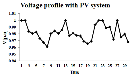
Figure 11 depicts the thirty bus systems with a PV system. The arrow points to the location of the PV device. Figure 12 depicts the voltage profile of the MVO-tuned device.
Figure 11. Single line representation of 30 node test network with a PV
6.1 PV based analysis on voltage profile, active and reactive powers
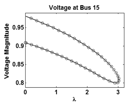
Figure 12. Voltage outline of the network with a PV network tuned by MVO
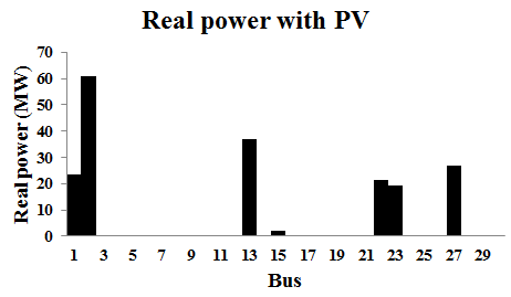
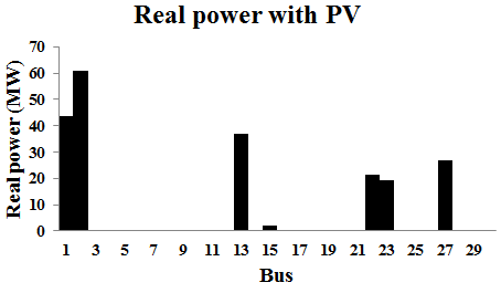
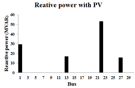
Figures 13 and 14 depict the active and reactive power profiles of the device with PV network, respectively. Figure 15 depicts the load capacity curve of the unit. In this case, the load capacity peaked at 3.0194. Table 7 lists the parameters of the unit with PV network. Table 8 shows the total generation and losses.
Figure 13. Active power profile of the unit with PV network
Figure 14. Reactive power profile of the unit with PV network
Figure 15. Load ability curve of the unit with PV network
Table 7. Load capacity curve of the unit with PV network
|
Bus No |
Volt in p.u |
P in p.u |
Q in p.u |
|
1 |
1.00000 |
23.65326 |
-0.44835 |
|
2 |
1.00000 |
60.97000 |
31.5634 |
|
3 |
0.98339 |
0.00000 |
0.00000 |
|
4 |
0.98038 |
0.00000 |
0.00000 |
|
5 |
0.98251 |
0.00000 |
0.00000 |
|
6 |
0.97345 |
0.00000 |
0.00000 |
|
7 |
0.96757 |
0.00000 |
0.00000 |
|
8 |
0.96090 |
0.00000 |
0.00000 |
|
9 |
0.98058 |
0.00000 |
0.00000 |
|
10 |
0.98436 |
0.00000 |
0.00000 |
|
11 |
0.98058 |
0.00000 |
0.00000 |
|
12 |
0.98554 |
0.00000 |
0.00000 |
|
13 |
1.00000 |
37.00000 |
11.3033 |
|
14 |
0.97696 |
0.00000 |
0.00000 |
|
15 |
0.98103 |
2.26000 |
0.00000 |
|
16 |
0.97740 |
0.00000 |
0.00000 |
|
17 |
0.97683 |
0.00000 |
0.00000 |
|
18 |
0.96890 |
0.00000 |
0.00000 |
|
19 |
0.96558 |
0.00000 |
0.00000 |
|
20 |
0.96938 |
0.00000 |
0.00000 |
|
21 |
0.99337 |
0.00000 |
0.00000 |
|
22 |
1.00000 |
21.59000 |
39.66548 |
|
23 |
1.00000 |
19.20000 |
7.54588 |
|
24 |
0.98861 |
0.00000 |
0.00000 |
|
25 |
0.99023 |
0.00000 |
0.00000 |
|
26 |
0.97221 |
0.00000 |
0.00000 |
|
27 |
1.00000 |
26.91000 |
10.58057 |
|
28 |
0.97499 |
0.00000 |
0.00000 |
|
29 |
0.97960 |
0.00000 |
0.00000 |
|
30 |
0.96820 |
0.00000 |
0.00000 |
Table 8. Total generation and losses of the unit with PV network
|
|
Generation |
Load |
Losses |
|
Watt power (MW) |
191.58 |
189.20 |
2.38 |
|
Wattles power (MVAR) |
100.21 |
107.20 |
6.99 |
6.2 10% and 20% rises in load with PV system
Figure 16 shows the voltage profile of the unit with PV network with a load increase of 10%. In this case, the voltage peaked at 1. The active and reactive power profiles of the unit with PV network are displayed in Figures 17 and 18, respectively. Figure 19 depicts the load capacity curve of the unit. In this case, the highest load capacity was 1.8254. Table 9 lists the parameters of the unit with PV network with a load increase of 10%. Table 10 shows the total generation and losses in this case.
Figure 16. Voltage profile of the unit with PV network-a load increase of 10%
Figure 17. Active power profile of the unit with PV network-a load increase of 10%
Figure 18. Reactive power profile of the unit with PV network-a load increase of 10%
Figure 19. Load capacity curve of the unit with PV network-a load increase of 10%
Table 9. Parameters of the unit with PV network-a load increase of 10%
|
Bus No |
Volt in p.u |
P in p.u |
Q in p.u |
|
1 |
1.00000 |
43.67678 |
29.3395 |
|
2 |
0.97255 |
60.97000 |
0.00000 |
|
3 |
0.95964 |
0.00000 |
0.00000 |
|
4 |
0.95237 |
0.00000 |
0.00000 |
|
5 |
0.95083 |
0.00000 |
0.00000 |
|
6 |
0.94204 |
0.00000 |
0.00000 |
|
7 |
0.93219 |
0.00000 |
0.00000 |
|
8 |
0.92483 |
0.00000 |
0.00000 |
|
9 |
0.96347 |
0.00000 |
0.00000 |
|
10 |
0.97517 |
0.00000 |
0.00000 |
|
11 |
0.96347 |
0.00000 |
0.00000 |
|
12 |
0.97044 |
0.00000 |
0.00000 |
|
13 |
1.00000 |
37.00000 |
16.9548 |
|
14 |
0.95597 |
0.00000 |
0.00000 |
|
15 |
0.95803 |
2.26000 |
0.00000 |
|
16 |
0.96227 |
0.00000 |
0.00000 |
|
17 |
0.96407 |
0.00000 |
0.00000 |
|
18 |
0.94620 |
0.00000 |
0.00000 |
|
19 |
0.94432 |
0.00000 |
0.00000 |
|
20 |
0.95081 |
0.00000 |
0.00000 |
|
21 |
0.99037 |
0.00000 |
0.00000 |
|
22 |
1.00000 |
21.59000 |
53.2210 |
|
23 |
0.97108 |
19.20000 |
0.00000 |
|
24 |
0.97457 |
0.00000 |
0.00000 |
|
25 |
0.98295 |
0.00000 |
0.00000 |
|
26 |
0.95882 |
0.00000 |
0.00000 |
|
27 |
1.00000 |
26.91000 |
15.7109 |
|
28 |
0.94487 |
0.00000 |
0.00000 |
|
29 |
0.97256 |
0.00000 |
0.00000 |
|
30 |
0.95683 |
0.00000 |
0.00000 |
Table 10. Total generation and losses of the unit with PV network-a load increase of 10%
|
|
Generation |
Load |
Losses |
|
Watt power (MW) |
211.61 |
208.12 |
3.49 |
|
Wattles power (MVAR) |
115.23 |
117.92 |
2.69 |
In the presence of PV network, the voltage peaked at 1 if the load increased by 20%. In this case, the load capacity maximized at 1.2498. Table 11 lists the parameters of the unit with PV network with a load increase of 20%. Table 12 shows the total generation and losses in this case.
The system with MVO-tuned PV achieved better results than that without PV network, as evidenced by the relatively high load capacity and small active power losses. The two cases are compared in details in Tables 13 and 14.
Table 11. Parameters of the unit with PV network-a load increase of 20%
|
Bus No |
Volt in p.u |
P in p.u |
Q in p.u |
|
1 |
1.00000 |
87.92576 |
38.46728 |
|
2 |
0.97285 |
60.97000 |
0.00000 |
|
3 |
0.96014 |
0.00000 |
0.00000 |
|
4 |
0.95295 |
0.00000 |
0.00000 |
|
5 |
0.95125 |
0.00000 |
0.00000 |
|
6 |
0.94260 |
0.00000 |
0.00000 |
|
7 |
0.93271 |
0.00000 |
0.00000 |
|
8 |
0.92539 |
0.00000 |
0.00000 |
|
9 |
0.96373 |
0.00000 |
0.00000 |
|
10 |
0.97525 |
0.00000 |
0.00000 |
|
11 |
0.96373 |
0.00000 |
0.00000 |
|
12 |
0.97078 |
0.00000 |
0.00000 |
|
13 |
1.00000 |
37.0000 |
21.8577 |
|
14 |
0.95663 |
0.00000 |
0.00000 |
|
15 |
0.95930 |
2.26000 |
0.00000 |
|
16 |
0.96248 |
0.00000 |
0.00000 |
|
17 |
0.96418 |
0.00000 |
0.00000 |
|
18 |
0.94700 |
0.00000 |
0.00000 |
|
19 |
0.94489 |
0.00000 |
0.00000 |
|
20 |
0.95126 |
0.00000 |
0.00000 |
|
21 |
0.99039 |
0.00000 |
0.00000 |
|
22 |
1.00000 |
21.5900 |
67.9654 |
|
23 |
0.97192 |
19.2000 |
0.00000 |
|
24 |
0.97490 |
0.00000 |
0.00000 |
|
25 |
0.98308 |
0.00000 |
0.00000 |
|
26 |
0.95895 |
0.00000 |
0.00000 |
|
27 |
1.00000 |
26.9100 |
21.3741 |
|
28 |
0.94540 |
0.00000 |
0.00000 |
|
29 |
0.97256 |
0.00000 |
0.00000 |
|
30 |
0.95683 |
0.00000 |
0.00000 |
Table 12. Total generation and losses of the unit with PV network-a load increase of 20%
|
|
Generation |
Load |
Losses |
|
Watt power (MW) |
255.86 |
249.46 |
6.4 |
|
Wattles power (MVAR) |
149.66 |
141.36 |
8.3` |
Table 13. Comparison of maximum loading parameters
|
Method |
Devoid of PV network in p.u |
With PV network wield MVO in p.u |
|
Normal |
2.9859 |
3.0194 |
|
Load 10% increased |
1.8254 |
1.8542 |
|
Load 20 % increased |
1.2296 |
1.2498 |
Table 14. Comparison of active power losses
|
Method |
Devoid of the PV network watt power losses [MW] |
With PV network wield MVO watt power losses [MW] |
|
Normal |
2.44 |
2.38 |
|
Load 10% increased |
3.58 |
3.49 |
|
Load 20 % increased |
6.56 |
6.4 |
This paper studies the congestion control of the grid through CPF simulation, and proposes an algorithm to acquire the full load capacity while minimizing active power losses. The test results show that the MVO approach outperforms other cases without PV network in terms of load capacity and active power losses. The MVO algorithm can optimize the size of PV, and rationalize the loading parameters, thereby ensuring grid safety and eliminating network congestion.
|
Pgmin |
Power generation minimum in p.u. |
|
Pgmax |
Power generation maximum in p.u. |
|
Pg |
Power generation in p.u. |
|
Qgmin |
Reactive power minimum in p.u. |
|
Qgmax |
Reactive power maximum in p.u. |
|
Qg |
Reactive power generation in p.u. |
|
Vmin |
Minimum voltage in p.u. |
|
Vmax |
Maximum voltage in p.u. |
|
V |
Voltage phase in p.u |
|
$g_{i}(x)$ |
Solar generation at time t |
|
$S_{r}$ |
Rated value of solar |
|
$T_{r}$ |
Temperature reference |
|
$T_{a}$ |
Temperature ambient |
|
$i_{r r}^{t}$ |
Solar irradiance at time t |
|
$P_{n}$ |
Active power generation from number of generators |
|
t |
time |
|
n |
Number of generators |
|
$f_{n}\left(P_{g}^{n}\right)$ |
Active power generation cost for n number of generators |
|
Greek symbols |
|
|
$\alpha$ |
Coefficient of temperature |
|
$\delta$ |
Voltage phase angle |
|
$\lambda$ |
Loading parameter value |
|
$\Theta$ |
dimensionless temperature |
|
$\mu$ |
dynamic viscosity, kg. m-1.s-1 |
|
Subscripts |
|
|
$f_{x}$ |
Function for x number of buses |
|
f |
Function |
|
$f_{n}$ |
Cost function for n number of generators |
[1] Suganthi, S.T., Devaraj, D., Ramar, K., Thilagar, S.H. (2018). An improved differential evolution algorithm for congestion management in the presence of wind turbine generators. Renewable And Sustainable Energy Reviews, 81: 635-642. https://doi.org/10.1016/j.rser.2017.08.014
[2] Remha, S., Chettih, S., Arif, S. (2016). Optimal placement of different DG units in distribution networks based on voltage stability maximization and minimization of power losses. 8th International Conference on Modelling, Identification, and Control (ICMIC), pp. 867-873. https://doi.org/10.1109/ICMIC.2016.7804237
[3] Arief, A., Nappu, M.B. (2015). DG placement and size with continuation power flow method. International Conference on Electrical Engineering and Informatics (ICEEI), pp. 579-584. https://doi.org/10.1109/ICEEI.2015.7352566
[4] El Fadhel Loubaba Bekri, O., Fellah, M.K. (2015). Placement of wind farms for enhancing voltage stability based on continuation power flow technique. 3rd International Renewable and Sustainable Energy Conference (IRSEC), pp. 1-6. https://doi.org/10.1109/IRSEC.2015.7455028
[5] Mirjalili, S., Mirjalili, S.M., Hatamlou, A. (2016). Multi-verse optimizer: A nature-inspired algorithm for global optimization. Neural Computing and Applications, 27: 495-513. https://doi.org/10.1007/s00521-015-1870-7
[6] Sharma, V., Walde, P., Walde, A.S. (2020). Hourly congestion management by adopting distributed energy storage system using hybrid optimization. Journal of Electrical Systems, 16(2): 257-275. http://journal.esrgroups.org/jes
[7] Gope, S., Goswami, A.K., Tiwari, P.K., Deb, S. (2016). Rescheduling of real power for congestion management with integration of pumped storage hydro unit using firefly Algorithm. International Journal of Electrical Power & Energy Systems, 83: 434-442. https://doi.org/10.1016/j.ijepes.2016.04.048
[8] Deb, S., Gope, S., Goswami, A.K. (2015). Congestion management considering wind energy sources using evolutionary algorithm. Electric Power Components and Systems, 43(7): 723-732. https://doi.org/10.1080/15325008.2014.1002587
[9] Hooshmand, R.A., Morshed, M.J., Parastegari, M. (2015). Congestion management by determining optimal location of series FACTS devices using hybrid bacterial foraging and Nelder-Mead algorithm. Applied Soft Computing Journal, 28: 57-68. https://doi.org/10.1016/j.asoc.2014.11.032
[10] Kashyap, M., Kansal, S. (2017). Hybrid approach for congestion management using optimal placement of distributed generator. International Journal of Ambient Energy, 39(2): 132-142. https://doi.org/10.1080/01430750.2016.1269676
[11] Nappu, M.B., Arief, A., Bansal, R.C. (2014). Transmission management for congested power system: A review of concepts, technical challenges and development of a new methodology. Renewable and Sustainable Energy Reviews, 38: 572-580. https://doi.org/10.1016/j.rser.2014.05.089
[12] Thangalakshmi, S., Valsalal, P. (2016). Congestion management in restructured power systems with economic and technical considerations. Asian Journal of Information Technology, 15(12): 2079-2086. https://doi.org/10.36478/ajit.2016.2079.2086
[13] Verma, S., Mukherjee, V. (2016). Optimal real power rescheduling of generators for congestion management using a novel ant lion optimiser. IET Generation, Transmission & Distribution, 10(10), pp. 2548-2561. https://doi.org/10.1049/iet-gtd.2015.1555
[14] Khatavkar, V., Namjoshi, M., Dharme, A. (2016). Congestion management in deregulated electricity market using FACTS & Multi-objective optimization. Indian Control Conference (ICC), pp. 467-473. https://doi.org/10.1109/INDIANCC.2016.7441176
[15] Dehnavi, E., Abdi, H. (2016). Determining optimal buses for implementing Demand Response as an effective congestion management method. IEEE Transactions on Power Systems, 32(2): 1537-1544. https://doi.org/10.1109/TPWRS.2016.2587843
[16] Vijayakumar, K. (2016). Optimal location of FACTS devices for congestion management in deregulated power systems. International Journal of Computer Applications (0975-8887), 16(6): 29-37. https://doi.org/10.5120/2015-1833
[17] Reddy, A.K., Singh, S.P. (2016). Congestion mitigation using UPFC. IET Generation, Transmission & Distribution, 10(10): 2433-2442. https://doi.org/10.1049/iet-gtd.2015.1199
[18] Ravindrakumar, K.B., Chandramohan, S. (2016). NSGA II based congestion management in deregulated power systems. Middle-East Journal of Scientific Research, 24(4): 1188-1193. https://doi.org/10.5829/idosi.mejsr.2016.24.04.23205