Shibam Manna | Tanmay Chowdhury | Asoke Kumar Dhar | Juan Jose Nieto*
© 2021 IIETA. This article is published by IIETA and is licensed under the CC BY 4.0 license (http://creativecommons.org/licenses/by/4.0/).
OPEN ACCESS
An attempt to model the human hair industry in the post-COVID-19 pandemic situation using mathematical modelling has been the goal of this article. Here we introduce a novel mathematical modelling using a system of ordinary differential equations to model the human hair industry as well as the human hair waste management and related job opportunities. The growth of human hair in the months of nationwide total lockdown has been taken into account and graphs have been plotted to analyze the effect of Lockdown in this model. The alternative employment opportunities that can be created for collecting excessive hair in the post-pandemic period has been discussed. A probable useful mathematical model and mechanism to utilize the migrant labours who became jobless due to the pandemic situation and the corresponding inevitable lockdown situation resulting out of that crisis has been discussed in this paper. We discussed the stability analysis of the proposed model and obtained the criteria for an optimal profit of the said model. Graphs have also been plotted to analyze the impact of the control parameter on the optimal profit.
mathematical modelling, human hair industry, lockdown effect due to COVID-19, economic impact, optimal profit
The COVID-19 pandemic has affected the entire world in many ways; health crisis and economic crisis are at the centre of all these crises. India is not an exception to all those crises borne out of the COVID-19 pandemic, where the economic crisis may have taken the upper hand. Millions of people became jobless both in the organized sector as well as in the unorganized sector; especially the daily wage migrant workers are at a serious threat of dying of starvation if they could survive the attack of novel corona-virus. In fact, not only India several other countries across the globe have witnessed a severe fall in GDP as well as economic loss due to the nationwide lock-down and related shut down in many production industries. In this premise, we look for alternative opportunities that may be created to boost up the economy.
Human hair can be treated as one of the most versatile natural resources available, which is used not only to produce wigs, weaves etc., but also used to produce calligraphy brushes, amino acid and to clean oil spills etc. In fact, from the past histories of economic downfalls it can be inferred that during the 2008 global economic crisis, it was the human hair industry that grew by 8% as compared to the other sectors [1]. According to an estimate [1], the current net worth of the global human hair industry is 7B USD and is estimated to rose up to 10B USD by the next three years.
So the human hair industry could probably be an alternative option in the post-pandemic period to deal with the said issue. In several countries across the globe, many celebrities spend millions of dollars on the wig and other products made of natural human hair for beautification. Patients suffering from cancer also use wigs to make up hair loss due to chemotherapy. Thus the human hair industry is one of the fastest-growing industries in the world. Earlier, people used to buy synthetic hair wigs made of animal hairs [2]. But now a days the demand for natural Remy hair is increasing day by day. Mainly the people from South India offer their hair to Lord Balaji as a part of their religious belief, which is one of the primary sources of Remy hair in India. This Remy hair is considered as the best quality hair for international export across the globe. Tirupati Balaji is one of the temples in India, which collects millions of dollars per years from the e-auction of hair. Also, village hair that comes from the combs and brushes of women is another degraded quality hair which is exported all around the globe for a lesser price. Another significant characteristic of human hair is that it is protein-rich [3] so it could be utilized as a primary raw material for Amino acid production [4, 5]. In this way, we could turn human hair waste that comes from sweeping off the floors of barbershops as well as the village hair into wealth [6] and it plays a significant role in waste management.
For all the above reasons, this sector is an important area that needs to be explored to perform research works from several aspects of science, technology, management and economics and very few research works have been published till date. In fact, our proposed model may probably be the first model that analyzes the mathematical aspects of this sector.
We divide the hairs into two categories of population, namely h1 and h2 category, based on their sizes [7]. In the first category (h1), we consider the population with hair size between 0 to 10 inches and in the second category (h2), we consider the population with hair size greater than 10 inches. In h1 category we basically consider the male, child and female teenage population for a while and in the h2 category we consider the female population of the age group 20-60 years. In our proposed model without control, we have considered the primary source of hair from the devotees of temples, who fully shave their hair and offer it to Lord Balaji [7]. The hair sizes greater than 10 inches are very much valuable which is called the natural Remy hair and often termed as “black gold”. Let us denote the population of collectors by C, in this category we consider both the barbers of temples as well as saloons including the collectors of village hair that is derived from the hair combs and brushes of women and the barber hair (“Thuku”) that comes from the sweepings off the floors from saloons [8]. There is a possible employment opportunity in this category since it does not require skilled labours. So the jobless migrant workers could be employed as collectors in this sector. In the optimal profit problem, we consider the collections from the temple offerings of devotees as well as the degraded quality village hair and barber hair. For the simplicity of the model, we do not discriminate between the barbers of saloons and temples and the collectors of village hair, “Thuku”. A schematic diagram has been presented in the Figure 1.
Figure 1. A diagram of the proposed white box model
Here we describe the model parameters as,
r1 is the population growth rate of h1,
k1 is the carrying capacity of the h1 population,
r2 is the population growth rate of C,
k2 is the carrying capacity of the C population (evidently, the carrying capacity of collector population is much less than that of the h1 population, i.e., $k_{2} \ll k_{1}$),
α is the rate of transmission from h1 to h2 category which is proportional to the growth rate of human hair (the effect of Lockdown can be considered here),
β the rate at which the transmission from h2 to h1 category occurs due to the collection of hair i.e, the rate collection of hair,
μ the rate at which new collectors are joining in the category C population, seeing the employment opportunity.
We have also neglected the hair from the collectors themselves. Thus our proposed model is as follows,
$\frac{d h_{1}}{d t}=r_{1} h_{1}\left(1-\frac{h_{1}}{k_{1}}\right)-\alpha h_{1}+\beta h_{2} C$ (1)
$\frac{d h_{2}}{d t}=\alpha h_{1}-\beta h_{2} C$ (2)
$\frac{d C}{d t}=r_{2} C\left(1-\frac{C}{k_{2}}\right)+\mu C\left(h_{1}+h_{2}\right)$ (3)
Along with the initial conditions h1(0)≥0, h2(0)≥0, C(0)>0.
In this section, we discuss the existence of solutions, equilibrium points of the system and their stability.
Theorem 1: The solutions of the proposed system subject to the initial conditions exist in the time interval [0, ∞) and they are +ve, i.e., h1(t)≥0, h2(t)≥0, C(t)>0 for all t≥0.
Proof: It can be easily verified that the R.H.S. of the system of Eqns. (1)-(3) are locally continuous as well as locally Lipschitz; therefore, the solution (h1(t), h2(t), C(t)) of our proposed model exists and unique on [0, ∞). From (1) on integration between the time limits 0 to t, we find that
$h_{1}(t)=h_{1}(0) \exp \left[\int_{0}^{t}\left\{r_{1}\left(1-\frac{h_{1}}{k_{1}}\right)-\alpha+\frac{\beta h_{2} C}{h_{1}}\right\} \mathrm{d} t\right]\geq 0$ (4)
In a similar manner, we obtain from Eqns. (2) and (3),
$h_{2}(t)=h_{2}(0) \exp \left[\int_{0}^{t}\left\{\frac{\alpha h_{1}}{h_{2}}-\beta C\right\} \mathrm{d} t\right] \geq 0$ (5)
$C(t)=C(0) \exp \left[\int_{0}^{t}\left\{r_{2}\left(1-\frac{C}{k_{2}}\right)+\mu\left(h_{1}+h_{2}\right)\right\} \mathrm{d} t\right]>0$ (6)
Therefore we find that h1(t)≥0, h2(t)≥0, C(t)>0 for all t≥0. Hence the proof.
Theorem 2: The solutions of the proposed system subject to the initial conditions are bounded.
Proof: From Eqns. (1) and (2) we have,
$\frac{d h_{1}}{d t}+\frac{d h_{2}}{d t}=r_{1} h_{1}\left(1-\frac{h_{1}}{k_{1}}\right)$ (7)
which is clearly bounded as $t \rightarrow \infty$ [9]. Therefore let us suppose that as $t \rightarrow \infty$,
$h_{1}(t)+h_{2}(t) \leq M_{1}$ (8)
M1 being upper bound in this case. Then from Eq. (3), we obtain
$\frac{d C}{d t} \leq r_{2} C\left(1-\frac{C}{k_{2}}\right)+\mu C M_{1}=\left(r_{2}+\mu M_{1}\right) C\left[1-\frac{r_{2} C}{k_{2}\left(r_{2}+\mu M_{1}\right)}\right]$ (9)
Thus as before we find that as $t \rightarrow \infty$,
$C(t) \leq \frac{k_{2}\left(r_{2}+\mu M_{1}\right)}{r_{2}}=M$ (10)
M being the upper bound in this case [10]. Therefore we find that h1(t), h2(t) and C(t) are bounded as $t \rightarrow \infty$. This concludes the proof.
Now, let us find the equilibrium points of the system and study the stability analysis of the system at these equilibrium points. To find the equilibrium points we equate the R.H.S. of (1)-(3) (considering C>0) to zero and obtain two equilibrium points namely E1(0,0,k2), and $E_{2}\left(h_{1}^{*}, h_{2}^{*}, C^{*}\right)$, where,
$h_{1}^{*}=k_{1}, h_{2}^{*}=\frac{\sqrt{\beta^{2} k_{2}^{2}\left(k_{1} \mu+r_{2}\right)^{2}+4 k_{1} k_{2} r_{2} \mu \alpha \beta}-\left(k_{1} \mu+r_{2}\right) \beta k_{2}}{2 \mu \beta k_{2}}$, $C^{*}=\frac{\sqrt{\beta^{2} k_{2}^{2}\left(k_{1} \mu+r_{2}\right)^{2}+4 k_{1} k_{2} r_{2} \mu \alpha \beta}+\left(k_{1} \mu+r_{2}\right) \beta k_{2}}{2 \beta r_{2}}$.
To find the nature of the equilibrium point E1(0,0,k2), we calculate the Jacobian matrix at E1 given below,
$J_{E_{1}}=\left[\begin{array}{ccc}r_{1}-\alpha & \beta k_{2} & 0 \\ \alpha & -\beta k_{2} & 0 \\ \mu k_{2} & \mu k_{2} & r_{2}\end{array}\right]$
The characteristic equation around the equilibrium point E1(0,0,k2) is
$\left(\lambda+r_{2}\right)\left\{\lambda^{2}+\left(\beta k_{2}+\alpha-r_{1}\right) \lambda-\beta k_{2} r_{1}\right\}=0$ (11)
Using Descartes’ rule of sign we find that Eq. (11) has two negative real roots and one positive real root, since all the parameters of the dynamical system (1)-(3) are positive reals. Thus we conclude that the equilibrium point E1(0,0,k2) is unstable, and we arrive at the following theorem,
Theorem 3: The equilibrium point E1(0,0,k2) of the proposed system exists and it is unstable.
Let us now look for the stability analysis of the nontrivial equilibrium point $E_{2}\left(h_{1}^{*}, h_{2}^{*}, C^{*}\right)$. To find the nature of the equilibrium point$E_{2}\left(h_{1}^{*}, h_{2}^{*}, C^{*}\right)$, we calculate the Jacobian matrix at $E_{2}$ in a similar manner, which given below
$J_{E_{2}}=\left[\begin{array}{ccc}r_{1}-\frac{2 r_{1} h_{1}^{*}}{k_{1}}-\alpha & \beta C^{*} & \beta h_{2}^{*} \\ \alpha & -\beta C^{*} & -\beta h_{2}^{*} \\ \mu C^{*} & \mu C^{*} & r_{2}-\frac{2 r_{2} C^{*}}{k_{2}}+\mu\left(h_{1}+h_{2}\right)\end{array}\right]$
The characteristic equation around the equilibrium point $E_{2}\left(h_{1}^{*}, h_{2}^{*}, C^{*}\right)$ is
$\lambda^{3}+A_{1} \lambda^{2}+A_{2} \lambda+A_{3}=0$ (12)
where, $A_{1}=\alpha+\beta C^{*}+r_{1}+\frac{r_{2} C^{*}}{k_{2}}, A_{2}=\left(\alpha+\beta C^{*}\right) \frac{r_{2} C^{*}}{k_{2}}+r_{1}\left(\beta C^{*}+\frac{r_{2} C^{*}}{k_{2}}\right), A_{3}=\frac{r_{1} r_{2} c^{* 2}}{k_{2}}$. It has been observed from the characteristic Eq. (12) that all the coefficients A1, A2, A3 as well as the expression A1A2-A3 are positive for any positive parameter values of the system. Thus employing the Routh-Hurwitz criteria, we arrive at the conclusion that our proposed dynamical system is locally asymptotically stable around the nontrivial equilibrium point $E_{2}\left(h_{1}^{*}, h_{2}^{*}, C^{*}\right)$. Based on these deductions, we state the following theorem:
Theorem 4: The nontrivial equilibrium point $E_{2}\left(h_{1}^{*}, h_{2}^{*}, C^{*}\right)$ of the proposed system exists and is locally asymptotically stable.
Here we focus on the time variation of the control parameter β(t) which is mainly associated with the collection rate of temple hair from the devotees of h2 category. Basically we consider β(t) being the rate at which the devotees of h2 population fully shaved their head at temples and move to h1 population. Additionally, we have considered that a constant fraction (ϵ) of both the population h1 and h2 contribute to the profit function by degraded quality hair that comes from the sweepings of saloons (“Thuku”) and village hair collected from the comb and brushes of women. We have considered this later category of degraded hair since it is easily available and serves as the prime raw material for Amino Acid production and is crucial to be included in the profit functional. Finally, we have assigned a constant cost γ to the population category C(t) for the collection of hair, which can be considered as the monthly income per collector. Here ρ1 is associated with normalized selling price of h2 category hair per collector per month.
Thus, we have constructed the objective functional as,
$P=\int_{0}^{t_{f}}\left[\rho_{1} \beta(t) C+\epsilon\left(h_{1}+h_{2}\right)-\gamma C\right] \mathrm{d} t$ (13)
Here we have constructed the objective functional linear in the control parameter, so it can be easily verified that an optimal control and associated optimal states exist using standard results [11]. Now we have to maximize the profit functional for the optimal value of the control parameter $\beta^{*}(t)$ such that
$P\left(\beta^{*}(t)\right)=\operatorname{maxP}(\beta), \beta \in \Omega$ (14)
where, $\Omega=\left\{\beta(t): 0 \leq a \leq \beta(t) \leq b, 0 \leq t \leq t_{f}, \beta(t)\right.$ being Lebesgue measurable}. Let us now employ the Pontryagin’s maximal principle [11-13] to obtain necessary conditions for optimal control. The Lagrangian is given as
$L(\beta)=\rho_{1} \beta(t) C(t)+\epsilon\left(h_{1}(t)+h_{2}(t)\right)-\gamma C(t)$ (15)
and the corresponding Hamiltonian is defined as
$H\left(\beta, \lambda_{1}, \lambda_{2}, \lambda_{3}\right)=L(\beta)+\lambda_{1}(t) \frac{d h_{1}}{d t}+\lambda_{2}(t) \frac{d h_{2}}{d t}+\lambda_{3}(t) \frac{d C}{d t}$ (16)
Here $\lambda_{i}$, (i=1,2,3) are adjoint variables corresponding to the states h1, h2 and C, respectively. Thus we have,
$\frac{d \lambda_{1}}{d t}=-\frac{\partial H}{\partial h_{1}}=-\lambda_{1}\left(r_{1}-\frac{2 r_{1} h_{1}}{k_{1}}-\alpha\right)-\alpha \lambda_{2}-\mu C \lambda_{3}-\epsilon$ (17)
$\frac{d \lambda_{2}}{d t}=-\frac{\partial H}{\partial h_{2}}=-\beta C \lambda_{1}+\beta C \lambda_{2}-\mu C \lambda_{3}-\epsilon$ (18)
$\frac{d \lambda_{3}}{d t}=-\frac{\partial H}{\partial C}=-\beta h_{2} \lambda_{1}+\beta h_{2} \lambda_{2}-\lambda_{3}\left[r_{2}-\frac{2 r_{1} C}{k_{2}}-\mu\left(h_{1}+h_{2}\right)\right]+\gamma-\rho_{1} \beta$ (19)
where, adjoint variables $\lambda_{i}(i=1,2,3)$ satisfy the transversality conditions
$\lambda_{i}\left(t_{f}\right)=0$, for $i=1,2,3$ (20)
Now, to maximize the Hamiltonian with respect to the control parameter β(t), we find that the Hamiltonian is linear in control variable β(t), so the optimal control may be bang-bang or singular. So we obtain the switching function as
$\Psi(t)=\frac{\partial H}{\partial \beta}=\rho_{1} C+C h_{2}\left(\lambda_{1}-\lambda_{2}\right)$ (21)
Here, singular control occurs when $\Psi(t)$ vanishes on nontrivial time interval. To obtain the singular case, we take $\frac{\partial H}{\partial \beta}=0$ on some nontrivial time interval. Thus we have,
$0=\frac{d}{d t}\left(\frac{\partial H}{\partial \beta}\right)=\rho_{1} \frac{d C}{d t}+\left(\frac{d \lambda_{1}}{d t}-\frac{d \lambda_{2}}{d t}\right) C h_{2}+\left(\lambda_{1}-\lambda_{2}\right)\left(C \frac{d h_{2}}{d t}+h_{2} \frac{d C}{d t}\right)$ (22)
Substituting the essential values in (22), we obtain an expression given below, which is free from the control parameter β(t) explicitly,
$\rho_{1}\left[r_{2} C\left(1-\frac{C}{k_{2}}\right)+\mu C\left(h_{1}+h_{2}\right)\right]+C h_{2}\left[\alpha\left(\lambda_{1}-\lambda_{2}\right)-\lambda_{1}\left(r_{1}-\frac{2 r_{1} h_{1}}{k_{1}}\right)\right] +\left(\lambda_{1}-\lambda_{2}\right)\left[r_{2} C h_{2}\left(1-\frac{C}{k_{2}}\right)\right. \left.+\mu C h_{2}\left(h_{1}+h_{2}\right)+\alpha C h_{1}\right]=0$ (23)
Thus we calculate $0=\frac{d^{2}}{d t^{2}}\left(\frac{\partial H}{\partial \beta}\right)=\beta(t) \phi_{1}(t)+\phi_{2}(t)$, where
$\phi_{1}(t)=\alpha C^{2}\left(\lambda_{1}-\lambda_{2}\right)\left(h_{1}+h_{2}\right)+C^{2} h_{2}\left\{\lambda_{1} r_{1} \frac{2 \lambda_{1} r_{1}}{k_{1}}\left(h_{1}-h_{2}\right)\right\}$ (24)
$\phi_{2}(t)=\left[r_{2} C\left(1-\frac{c}{k_{2}}\right)+\mu C\left(h_{1}+h_{2}\right)\right]$
$\left[\rho_{1} r_{2}\left(1-\frac{2 c}{k_{2}}\right)+\rho_{1} \mu\left(h_{1}+h_{2}\right)+2 C\left\{\alpha\left(\lambda_{1}-\lambda_{2}\right)\right.\right.$
$\left.-\lambda_{1}\left(r_{1}-\frac{2 r_{1} h_{1}}{k_{1}}\right)\right\}\left(\lambda_{1}-\lambda_{2}\right)\left(r_{2} h_{2}-\frac{2 C r_{2} h_{2}}{k_{2}}+\mu h_{1} h_{2}\right.\left.\left.+\mu h_{2}^{2}+\alpha h_{1}\right)\right]$
$+2 \alpha C h_{1}\left[\alpha\left(\lambda_{1}-\lambda_{2}\right)-\lambda_{1}\left(r_{1}-\frac{2 r_{1} h_{1}}{k_{1}}\right)\right]$
$+\rho_{1} \mu C r_{1} h_{1}\left(1-\frac{h_{1}}{k_{1}}\right)+C h_{2}\left[\alpha^{2}\left(\lambda_{1}-\lambda_{2}\right)\right.$
$-\left(r_{1}-\frac{2 r_{1} h_{1}}{k_{1}}\right)\left\{\alpha\left(2 \lambda_{1}-\lambda_{2}\right)-\lambda_{1}\left(r_{1}-\frac{2 r_{1} h_{1}}{k_{1}}\right)\right.$
$\left.\left.-\mu C \lambda_{3}-\epsilon\right\}\right]+\left(\lambda_{1}-\lambda_{2}\right)\left(\alpha C h_{1} r_{1}-\frac{R_{2} C^{2} \alpha h_{1}}{k_{2}}\right. \left.+\alpha \mu C h_{1}^{2}+2 \alpha \mu C h_{1} h_{2}\right)$
$+\left\{r_{1} h_{1}\left(1-\frac{h_{1}}{k_{1}}\right)-\alpha h_{1}\right\}|\left\{2 \lambda_{1} r_{1} C h_{2}\left(\lambda_{1}-\lambda_{2}\right)\right.( \alpha C\left.\left.+\mu C h_{2}\right)\right\}$ (25)
Thus, we obtain the expression of $\beta(t)$ as $\beta(t)=-\frac{\phi_{2}(1)}{\phi_{1}(t)}$, where $\phi_{1}(t) \neq 0$ and $a \leq \beta(t) \leq b$.
Now, to satisfy the Generalized Legendre-Clebsch Condition [14, 15] for singular control to be optimal, we need, $\frac{\partial}{\partial \beta}\left[\frac{d^{2}}{d t^{2}}\left(\frac{\partial H}{\partial \beta}\right)\right]>0$, i.e., $\phi_{1}(t)>0 .$ Hence the control is optimal when $\phi_{1}(t)>0$ and $a \leq \beta(t) \leq b$.
We have estimated the normalized parameter values using several papers and news reports [16-19] and provide them in the Table 1. Here, the dimension of $r_{1}, r_{2}, \alpha, \beta$ and $\mu$ is $\frac{1}{[\text { Time }]}$ and k1, k2 are dimensionless parameters.
Table 1. Normalized parameter values
|
Parameters |
Normalized values |
|
$r_{1}$ |
0.1 |
|
$k_{1}$ |
0.85 |
|
$r_{2}$ |
0.08 |
|
$k_{2}$ |
0.045 |
|
$\alpha$ |
0.0047 |
|
$\beta$ |
0.65 |
|
$\mu$ |
0.0014 |
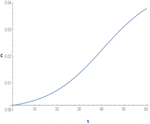
Using these values, we have plotted the graphs of h1, h2 and C with respect to time t (taken in months), taking the normalized initial values h1(0)=0.09, h2(0)=0.0083 and C(0)=0.0017 with the help of Wolfram Mathematica, as shown in Figure 2.
During the period of total Lockdown, the temples, as well as the barbershops, were closed and no collections were made. So if we neglect the small amount of wastage of hair then there must be a shift from the population category h1 to category h2 population due to continuous hair growth. Now, we consider that during the period of lockdown there is a 20% increment on the normalized initial value of h2 in every 100 days as provided in the following Table 2. Based on this assumption we have plotted the graph of h2 with respect to time t (taken in months) in Figure 3, taking all other normalized initial conditions and parameter values to be identical as before. From Figure 3 we see that due to the Lockdown effect population of h2 increases.
Table 2. Change in normalized initial value of h2 due to the Lockdown effect
|
Lockdown in days |
Normalized initial value of $\boldsymbol{h}_{2}$ |
|
1 |
0.0083 |
|
100 |
0.01 |
|
200 |
0.0117 |
We have also investigated the effect of harvesting parameter β(t) in the profit function P(t) using the Wolfram Mathematica and MATLAB software, considering the normalized parameter values $\rho_{1}=2.656, \epsilon=0.200025$ and $\gamma=1.36$. In Figure 4 we have plotted the profit function in case of optimal harvesting as well as the absence of optimal harvesting taking a constant value β=0.65.
Figure 2. Plots of h1(t), h2(t) and C(t), t in months
Figure 3. Plot of h2(t) considering the effect of Lockdown for several initial values of h2(t) (for red h2(0)=0.0083, for blue h2(0)=0.01 and for green h2(0)=0.0117, t being taken in months
Figure 4. Plot of P(t) considering the effect of harvesting parameter β(t) (indicated in green) as well as in the absence of optimal harvesting parameter, assigning only a constant value of β=0.65 (indicated in blue)
In this paper, we have discussed both analytically and numerically the mathematical model of the human hair industry. To analyze the mathematical aspects, we kept our model simple. However, this fundamental introductory model could probably be a stepping stone on an otherwise unexplored arena of applied mathematical modelling and serve as a bridge for several branches of science, technology and economics. This article also finds future employment opportunities of the jobless migrant workers as collectors of human hair in the post-pandemic period. Figure 2 depicts that h1(t), h2(t) and C(t) grow logistically. It can be inferred from Figure 3 that due to nationwide total Lockdown, there is an increment in hair and eventually an increment in the h2 category population. We have also obtained the criteria for optimal profit. From Figure 4 we observed that due to the control applied in the harvesting parameter β(t), derived with the help of (24) and (25), the profit function P(t) maximizes. Thus our model could find an alternative solution for the employment of the jobless migrant workers as well as providing an economic boost and an alternative way to human hair waste management in the post-pandemic period in India.
The work of Prof. Juan Jose Nieto has been partially supported by the Agencia Estatal de Investigación (AEI) of Spain under Grant MTM2016-75140-P, cofinanced by the European Community fund FEDER, as well as by Instituto de Salud Carlos III, grant COV20/00617. and by Xunta de Galicia grant ED431C 2019/02 for Competitive Reference Research Groups (2019-22). Shibam Manna is thankful to IIEST, Shibpur, India, for providing institute fellowship to him.
|
h1 |
Population of hair size (0-10) inches. |
|
h2 |
Population of hair size greater than 10 inches. |
|
C |
Population of hair collectors |
|
k1 |
is the carrying capacity of the h1 population |
|
k2 |
is the carrying capacity of the C population |
|
r1 |
is the population growth rate of h1 |
|
r2 |
is the population growth rate of C, |
|
Greek symbols |
|
|
$\alpha$ |
is the rate of transmission from h1 to h2 category, which is proportional to the growth rate of human hair |
|
$\beta$ |
the rate at which the transmission from h2 to h1 category occurs due to the collection of hair, i.e., the rate collection of hair |
|
β(t) |
the control parameter |
|
γ |
cost for the collection of hair |
|
ϵ |
a constant fraction of profit that comes from both the population h1 and h2 Thuku and village hair |
|
µ |
the rate at which new collectors are joining in the category C population |
|
ρ1 |
the normalized selling price of $h_{2}$ category hair per collector per month |
|
λ1 |
adjoint variables corresponding to the state h1 |
|
λ2 |
adjoint variables corresponding to the state h2 |
|
λ3 |
adjoint variables corresponding to the state C |
[1] https://thehustle.co/the-economics-of-the-human-hair-trade/.
[2] Wilson, N., Thomson, A., Moore-Millar, K., Ijomah, W. (2019). Capturing the life cycle of false hair products to identify opportunities for remanufacture. Journal of Remanufacturing, 9(3): 235-256. https://doi.org/10.1007/s13243-019-0067-0
[3] Rashaid, A.H., Harrington, P.B., Jackson, G.P. (2015). Amino acid composition of human scalp hair as a biometric classifier and investigative lead. Analytical Methods, 7(5): 1707-1718. https://doi.org/10.1039/C4AY02588A
[4] Patil, S.B., Shreya, K., Kruti, S. (2020). Extraction of Amino acids from Human Hair" Waste" and Used as a Natural Fertilizer. Journal of Pharmaceutical Sciences and Research, 12(2): 271-278.
[5] Robbins, C.R., Kelly, C.H. (1970). Amino acid composition of human hair. Textile Research Journal, 40(10): 891-896. https://doi.org/10.1177%2F004051757004001005
[6] Gupta, A. (2014). Human hair “waste” and its utilization: gaps and possibilities. Journal of Waste Management. http://dx.doi.org/10.1155/2014/498018
[7] Tarlo, E. (2016). Entanglement: The secret lives of hair. Simon and Schuster.
[8] Jagannathan, K., Panchanatham, N. (2011). An overview of human hair business in Chennai. International Journal of Engineering and Management Sciences, 2(4): 199-204.
[9] Jana, S., Ghorai, A., Guria, S., Kar, T.K. (2015). Global dynamics of a predator, weaker prey and stronger prey system. Applied Mathematics and Computation, 250: 235-248. https://doi.org/10.1016/j.amc.2014.10.097
[10] Sharma, S., Samanta, G.P. (2016). Analysis of the dynamics of a tumor–immune system with chemotherapy and immunotherapy and quadratic optimal control. Differential Equations and Dynamical Systems, 24(2): 149-171. https://doi.org/10.1007/s12591-015-0250-1
[11] Fleming, W.H., Rishel, R.W. (2012). Deterministic and stochastic optimal control (Vol. 1). Springer Science & Business Media.
[12] Lenhart, S., Workman, J.T. (2007). Optimal Control Applied to Biological Models. CRC Press.
[13] Boltyanskiy, V.G., Gamkrelidze, R.V., Mishchenko, Y., Pontryagin, L.S. (1962). Mathematical Theory of Optimal Processes. CRC Press.
[14] Robbins, H.M. (1967). A generalized Legendre-Clebsch condition for the singular cases of optimal control. IBM Journal of Research and Development, 11(4): 361-372. https://doi.org/10.1147/rd.114.0361
[15] Krener, A.J. (1977). The high order maximal principle and its application to singular extremals. SIAM Journal on Control and Optimization, 15(2): 256-293. https://doi.org/10.1137/0315019
[16] Harkey, M.R. (1993). Anatomy and physiology of hair. Forensic Science International, 63(1-3): 9-18. https://doi.org/10.1016/0379-0738(93)90255-9
[17] Loussouarn, G., El Rawadi, C., Genain, G. (2005). Diversity of hair growth profiles. International Journal of Dermatology, 44: 6-9. https://doi.org/10.1111/j.1365-4632.2005.02800.x
[18] Loussouarn, G., Lozano, I., Panhard, S., Collaudin, C., El Rawadi, C., Genain, G. (2016). Diversity in human hair growth, diameter, colour and shape. An in vivo study on young adults from 24 different ethnic groups observed in the five continents. European Journal of Dermatology, 26(2): 144-154. https://doi.org/10.1684/ejd.2015.2726
[19] https://www.mospi.gov.in.