Asmaa Lakhdar* | Abdenbi Mimouni | Zineddine Azzouz
© 2021 IIETA. This article is published by IIETA and is licensed under the CC BY 4.0 license (http://creativecommons.org/licenses/by/4.0/).
OPEN ACCESS
The aim of this paper is to perform a parametric study in order to analyze factors having an effect on the vertical lightning field polarization to the CN-Tower in Canada, and estimate with numerical simulation, the horizontal distance for which the reversed polarity will occur. The calculation is performed using the Finite-Difference-Time-Domain technique in two dimensions (2D-FDTD), the spatial-temporal current propagation through the lightning channel and through the high structure is represented by the lumped-series voltage-source model. The obtained results show that the vertical electric lightning field behavior has a dual polarity, the transition from a negative waveform to a positive one is observed at different observation points localized near the elevated object influencing by each modification made to the tower-parameters, the medium conductivity and the return stroke speed value. These results can contribute to the understanding of the lightning-phenomenon and allow to solve the problems of electromagnetic compatibility.
electromagnetic compatibility, 2D-FDTD method, lightning to tall object, polarization reversal of the vertical electric lightning field
Scientists around the world have used a variety of experimental measurements to acquire lightning current data, such as the artificial triggered of lightning [1-3] and the instrumented elevated objects [4-11], in order to find solutions to the lighting electromagnetic coupling issues with the electrical systems and the electronic devises.
The first experimental measurement of lightning currents was done in 1953, at the Empire State Building (New York), where McEachron [12] discovered the existence of the ascending tracers.
In 1970, Berger [13] obtained the whole statistical description of lightning current parameters, on Mont-San Salvatore (Switzerland).
The use of the instrumented elevated objects has rapidly grown in the recent years, including the Ostankino high object in Russia [4], the CN-Tower installed in Toronto [14], the Peissenberg-Tower implanted in Germany [6], the Gaisberg-Tower in Salzburg [15], the Säntis-Tower on the Alps Mountain in Swiss [16] and the Skytree elevated structure in Tokyo [17].
Observation results concerned the instrumented elevated objects measurements provided that the lightning current and the associated electromagnetic field are heavily affected by the presence of tall object [4-6, 14-28], in particular, the vertical electric lightning field which exhibits a reversal polarity above and below the ground, close to the strike tower.
Mosaddeghi et al. [21] developed a mathematical equation in order to estimate the critical- radial distance of electric field polarity reversal to tall object, based on two theoretical explanations, the first one was provided in 1975, by Uman et al. [22], it concerned the general electromagnetic field equations for a perfect ground case, the second one is about the equation formulated in 2005, by Baba and Rakov [23], from the hypotheses proposed in 2001, by Thottappillil et al. [24].
Until now, this mathematical formulation [21] is unique and valid only for the case of perfect ground, also it depends solely on the bottom reflection tower coefficient and the height of the elevated structure.
The objective of this paper is to estimate the crucial observation point location in the r-direction, for where the vertical lightning electric field will be inverted and become totally positive, in the proximity of the CN-Tower in presence of conducting ground and analyze the influence of the tower-parameters, the medium conductivity and the return stroke speed value on the position of the polarity reversal of the vertical electric field.
This paper is organized as follows: In Section II, the 2D-FDTD method is briefly described, the section III is devoted to the mathematical models of lightning current and the vertical electric field to tall object, in section VI, we present the simulation parameters and numerical results which are accompanied by some observations and remarks, finally, general conclusion is given.
The rise of the numerical methods and the development of computers performances furnished to the researchers the opportunity to solve many complex physical phenomena.
In 1966, Yee [29] proposed the resolution of the Maxwell’s Eq. (1) and (2) by the Finite-Difference-Time-Domain method (FDTD).
$\nabla \times E=-\mu \frac{\partial H}{\partial t}$ (1)
$\nabla \times H=\sigma E+\varepsilon \frac{\partial E}{\partial t}$ (2)
The twin spatial and temporal discretization with the 2D-FDTD method in the cylindric coordinates of the derivation operators of Eq. (1) and (2) uses a centred finite difference scheme.
Eq. (3) showed the derivation operators of the magnetic field.as followings:
$\frac{\partial H \varphi}{\partial t}=\frac{1}{\mu}\left[\frac{\partial E z}{\partial r}-\frac{\partial E r}{\partial z}\right]$ (3)
The operator’s derivation of the horizontal and the vertical lightning electric-field are presented in Eq. (4) and (5) respectively.
$\sigma E_{r}+\varepsilon \frac{\partial E_{r}}{\partial t}=-\frac{\partial H_{\varphi}}{\partial z}$ (4)
$\sigma E_{z}+\varepsilon \frac{\partial E_{z}}{\partial t}=\frac{1}{r} \frac{\partial}{\partial r}\left(r H_{\varphi}\right)$ (5)
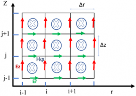
The 2D-FDTD structure consists on the discretization of the computation domain into small squares of dimension ∆r and ∆z, as showed in Figure 1.
Figure 1. Two-dimensional FDTD computing domain
The 2D-FDTD scheme converges to the solution if the point-wise error approaches towards zero [30], for the mutual steps-dimensions (spatial and temporal steps).
The convergence stability criterion is expressed as followings:
$\Delta t \leq \min \frac{(\Delta r, \Delta z)}{2}$ (6)
Like any algorithm, the domain of resolution must be bounded, this is accomplished by truncating the mesh and using absorbing boundary conditions (ABC).
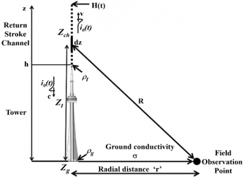
The adopted geometry for the calculation of the vertical electric field is illustrated in Figure 2.
Figure 2. Adopted geometry
The mathematical expression of the vertical electric field according to the Yee’s 2D-Finite- Difference approximations for Maxwell’s Eq. (1), (2) in the cylindrical coordinates system is written as followings:
$E_{z}^{n+1}\left(i, j+\frac{1}{2}\right)=\left(\frac{2 \varepsilon-\sigma \Delta t}{2 \varepsilon+\sigma \Delta t}\right) E_{z}^{n}\left(i, j+\frac{1}{2}\right)+$
$\frac{2 \Delta t}{(2 \varepsilon+\sigma \Delta t) r_{i} \Delta r} \times\left[\begin{array}{l}r_{i+(1 / 2)} \cdot H_{\varphi}^{n+(1 / 2)}\left(i+\frac{1}{2}, j+\frac{1}{2}\right)- \\ r_{i-(1 / 2)} \cdot H_{\varphi}^{n+(1 / 2)}\left(i-\frac{1}{2}, j+\frac{1}{2}\right)\end{array}\right]$ (7)
From Eq. (7) we observed that the principle of the time discretization in the Finite-Difference method is based on the Leap-Frog model, which makes the formulation of the magnetic and the radial electric field necessary in the calculation of the vertical electric-field.
Eqns. (8) and (9) present the mathematical formulas of the magnetic and the radial electric field respectively.
$H_{\varphi}^{n+1 / 2}\left(i+\frac{1}{2}, j+\frac{1}{2}\right)=H_{\varphi}^{n-1 / 2}\left(i+\frac{1}{2}, j+\frac{1}{2}\right)+$
$\frac{\Delta t}{\mu \Delta r}\left[\begin{array}{c}E_{z}^{n}\left(i+1, j+\frac{1}{2}\right)- \\ E_{z}^{n}\left(i, j+\frac{1}{2}\right)\end{array}\right]-\frac{\Delta t}{\mu \Delta z}\left[\begin{array}{c}E_{r}^{n}\left(i+\frac{1}{2}, j+1\right)- \\ E_{r}^{n}\left(i+\frac{1}{2}, j\right)\end{array}\right]$ (8)
The vertical electric field at the instant ‘n+1’ is calculated by using its previous value in the preceding step at the instant ‘n’. The same process for the magnetic field but at the instant ‘n+1/2’.
$E_{r}^{n+1}\left(i+\frac{1}{2}, j\right)=\left(\frac{2 \varepsilon-\sigma \Delta t}{2 \varepsilon+\sigma \Delta t}\right) E_{r}^{n}\left(i+\frac{1}{2}, j\right)-$
$\left(\frac{2 \Delta t}{(2 \varepsilon+\sigma \Delta t) \Delta z}\right) \times\left[\begin{array}{l}H_{\varphi}^{n+(1 / 2)}\left(i+\frac{1}{2}, j+\frac{1}{2}\right) \\ - \\ H_{\varphi}^{n+(1 / 2)}\left(i+\frac{1}{2}, j-\frac{1}{2}\right)\end{array}\right]$ (9)
At the source region of the computation [31], The vertical electric field at the zero point of the Z-direction (Figure 1) can be written as:
$\begin{aligned} E_{z}^{n+1}\left(0, j+\frac{1}{2}\right) &=\left(\frac{2 \varepsilon-\sigma \Delta t}{2 \varepsilon+\sigma \Delta t}\right) E_{z}^{n}\left(0, j+\frac{1}{2}\right) \\ &+\left(\frac{8 \Delta t}{(2 \varepsilon+\sigma \Delta t) \Delta r}\right) H_{\varphi}^{n+(1 / 2)}\left(\frac{1}{2}, j+\frac{1}{2}\right) \\ &-\left(\frac{4 \Delta t}{\pi \varepsilon_{0} \Delta r^{2}}\right) I\left(0, j+\frac{1}{2}\right) \end{aligned}$ (10)
From Eq. (10), the electric field is proportional to the lightning current element at height $\Delta z \cdot\left(j+\frac{1}{2}\right)$.
The model proposed by Baba and Rakov [32] based on the lumped-series voltage-source is used in the calculation to represent the return-stroke-current re-partition (Figure 2), this choice is justified by the fact that this engineering model reproduced the shapes and amplitudes of electromagnetic fields measured experimentally.
The spatial-temporal formulation of the return stroke current propagating inside the tower ($z^{\prime}$ lower than the height of the Tower, Figure 2) is exposed in the Eq. (11):
$i\left(z^{\prime}, t\right)=\left(\left(1-\rho_{t}\right) / 2\right)$
$\times \sum_{n=0}^{\infty}\left[\begin{array}{l}\rho_{t}^{n} \rho_{g}^{n} i_{S c}\left(h, t-\frac{h-z^{\prime}}{c}-\frac{2 n h}{c}\right) \\ + \\ \rho_{t}^{n} \rho_{g}^{n+1} i_{S C}\left(h, t-\frac{h-z^{\prime}}{c}-\frac{2 n h}{c}\right)\end{array}\right]$ (11)
The Eq. (12) showed the spatial-temporal expression of the return stroke current propagating through the lightning channel (z' upper than the height of the tower, Figure 2).
$i\left(z^{\prime}, t\right)=\left(\left(1-\rho_{t}\right) / 2\right)$
$\left[\begin{array}{l}i_{S C}\left(h, t-\frac{z^{\prime}-h}{v}\right) \\ + \\ \sum_{n=0}^{\infty} \rho_{t}^{n} \rho_{g}^{n-1}\left(1+\rho_{t}\right) i_{S C}\left(h, t-\frac{h-z^{\prime}}{v}-\frac{2 n h}{c}\right)\end{array}\right]$ (12)
h, ρt and ρg and are the height, the top and the bottom reflection coefficient of the tower respectively.
The mathematical formulation of the short-circuit current noted isc, related to the ideal-current measured on the top of the tower marked i0 is presented as followings:
$i_{s c}(t)=2 \times i_{0}(t)$ (13)
Heidler’s function for the ideal-current i0 is expressed as follows [33]:
$\begin{aligned} i_{0}(h, t) &=\frac{I_{01}}{\eta_{1}} \times\left(\frac{\left(t / \tau_{11}\right)^{n_{1}}}{1+\left(t / \tau_{11}\right)^{n}}\right) \times \exp \left(-t / \tau_{12}\right) \\ &+\\ & \frac{I_{02}}{\eta_{2}} \times\left(\frac{\left(t / \tau_{21}\right)^{n_{2}}}{1+\left(t / \tau_{21}\right)^{n_{2}}}\right) \times \exp \left(-t / \tau_{22}\right) \end{aligned}$ (14)
with η1 and η2 are calculate in Eqns. (15) and (16):
$\eta_{1}=\exp \left[\left(-\frac{\tau_{11}}{\tau_{12}}\right)\left(n_{1} \frac{\tau_{12}}{\tau_{11}}\right)^{1 / n_{1}}\right]$ (15)
$\eta_{2}=\exp \left[\left(-\frac{\tau_{21}}{\tau_{22}}\right)\left(n_{2} \frac{\tau_{22}}{\tau_{21}}\right)^{1 / n_{2}}\right]$ (16)
As mentioned previously, Mosaddeghi et al. [21] developed a mathematical expression presented in Eq. (17), in order to estimate the critical r-distance from the tower, where the change in polarity of the vertical electric field is produced.
$r_{c}=\left(1-\rho_{g}\right) \frac{h}{2}$ (17)
The Eq. (17) is applicate in the case of lighting strike to tall object in presence of perfect ground, it depends on the bottom reflection coefficient and the height of tower.
Other parameters are considered in this study such as finite ground conductivity, return stroke speed and tower parameters.
The instrumented elevated objects parameters are mentioned in Table 1 conforming to the proposed geometry (Figure 2).
Table 1. Elevated objects parameters
|
Instrumented tower name’s |
Height (m) |
Top reflection tower coefficient |
Bottom reflection tower coefficient |
|
Gaisberg Tower [34] |
100 |
-0.45 |
0.8 |
|
Peissenberg Tower [6] |
168 |
-0.53 |
0.7 |
|
CN Tower [14] |
553 |
-0.366 |
0.8 |
The simulated current parameters according to the Heidler's function (14) are: $I_{01}=10.7 k A, I_{02}=6.5 k A, \tau_{11}=0.25 \mu s, \tau_{12}=2.5 \mu s, \tau_{21}=2 \mu s, \tau_{22}=230 \mu s, n_{1}=2$ and $n_{2}=2$. The spatial steps for the r-axe and z-axe respectively in cylindrical coordinates system are: $\Delta r=\Delta z=1 m,$ the time steps $\Delta t=1 n s$.
The relative permitivity $\varepsilon_{r}=10$ when the ground conductivity σ set as 0.01 S/m and 0.001S/m. For the case of perfect ground $\varepsilon_{r}=1$.
The boundless computing domain must be truncated into a finite domain, in order to solve mathematical equations of the electromagnetic lightning field by the 2D-FDTD method, this is performed by using Absorbing Boundary Conditions (ABCs). The first-order Mur absorbing boundary conditions [30] are adopted in the computation to simulate the limitless surroundings.
4.1 Field polarization reversal to tall object in presence of conducting ground
In this section, we will estimate the crucial-distance value noted “rcd” corresponding to the transient’s field polarisation to tall object (CN, Peissenberg and Gaisberg Towers) in presence of conducting ground (σ=0.01 S/m).
The evaluated parameters for each tower are mentioned in Table 1. The return stroke speed is set as 1.5×10⁸ m/s.
The vertical electric field is calculated at different radial distance from the elevated object to better visualize the change in polarity of field for each tower separately, (bipolar, positive and the crucial distance for which the change of polarity is observed).
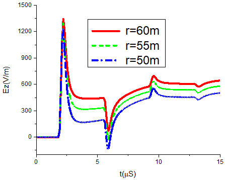
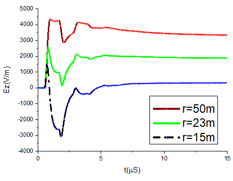
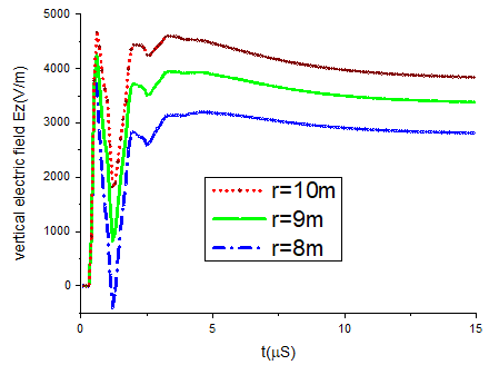
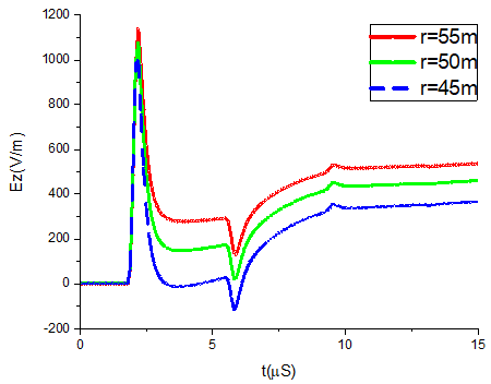
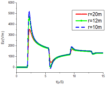
Figure 3. Vertical electric field polarization according to the CN -Tower height (h=553-m)
Figure 4. Vertical electric field sign according to the Peissenberg -Tower height (h=168-m)
Figure 5. Vertical electric field polarity inversion according to the Gaisberg -Tower height (h=100-m)
The crucial radial distance estimated by Eq. (17) for the elevated objects (553-m, 168-m and 100-m towers) is 55m, 25m and 10m respectively, however, in presence of conducting ground, we observed from Figure 3, that the field has a positive polarity at 60m from the CN tower, and a bipolar polarity at 55m.
From Figures 4 and 5, the field has a positive polarity at 23m from the 168-m tower and 9m from the 100-m tower.
Table 2 resume the crucial distance of field inversion waveform of our computation and of Eq. (17) respectively.
Table 2. Horizontal distance about the field inversion waveform corresponding to the height variation
|
h (m) |
553-m |
168-m |
100-m |
|
rcd(m) |
60 |
23 |
9 |
|
rcd(m) [21] |
55 |
25 |
10 |
4.2 Top reflection tower coefficient influencing on the field waveform polarity’s
To approximate the radial-distance for where the electric field will be reversed, we will modify the top reflection coefficient of the 553-m tower as shown in Table 3, with maintaining the ground conductivity of soil equal to 0.01S/m, the return stroke speed set as 1.5×10⁸ m/s and the bottom reflection coefficient set as 0.8.
Figure 6. Field waveform according to ρt = - 0.2
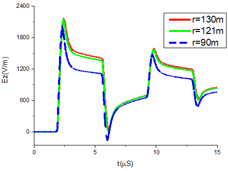
Figure 7. Field wave-shape according to ρt = - 0.8
From Figures 6 and 7, The crucial radial distance is observed at 50m and at 121m respectively from the 553-m tower.
As resume in Table 3, the inversion of field polarity’s is estimated at different radial distances according to each value of the top reflection tower coefficient.
The variation ratio of the inverted shape is about:10m, corresponding approximately to the percentage difference values of the top reflection coefficient (-0.2, -0.366) and around: 60m equivalent to the percentage subtraction between the two coefficients (-0.2, -0.8)
Table 3. Radial distance relating to the field transition sign according to the top reflection tower coefficient
|
ρt |
-0.2 |
-0.366 |
-0.8 |
|
rcd (m) |
50 |
60 |
121 |
4.3 Electric field polarity’s sensibility to the bottom reflection tower coefficient
We will procced with the same process as previously, by keeping the same parameters of the return stroke speed, the tower height and the ground conductivity, the top reflection tower coefficient set as -0.366. The bottom reflection tower coefficient is variated to visualize its effect on the field waveform polarization (in Table 4).
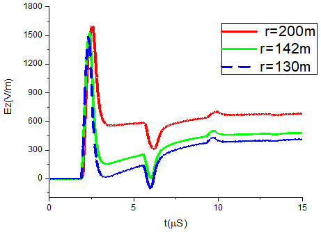
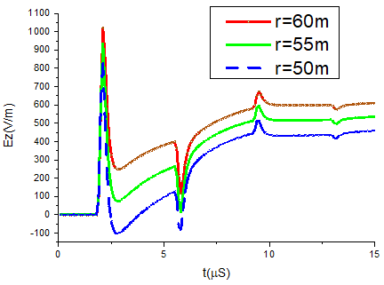
Figure 8. Electric field polarization according to ρg = 0.5
Figure 9. Electric field sign corresponding to ρg = 1
The field became positive further away from the 553-m tower, nearly to 142m when the bottom reflection coefficient is set as 0.5 (Figure 8), however, where we assumed a unit reflection coefficient, it turned out that the field transients to a positive form at very close radial distance (Figure 9) and field shape is clearly modified. The Table 4 reports the summary about the distance’s ranges in regards to the 553-m tower for which the reversion shape will occur.
Table 4. Crucial r-direction corresponding to the reversed field sign related to the bottom reflection coefficient variation
|
ρg |
0.5 |
0.8 |
1 |
|
rcd (m) |
142 |
60 |
12 |
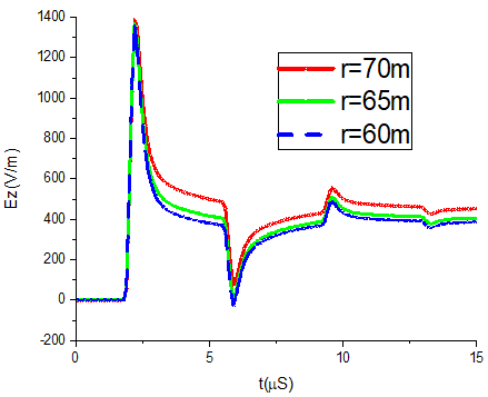
4.4 Field waveshape sensitivity to the ground conductivity
In order to visualized the impact of the ground conductivity on the field waveshape polarity, we kept the same parameters of the 553-m tower (see Table 1), the return stroke speed set as 1.5×10⁸ m/s, solely the electric ground conductivity is changed according to the Table 5.
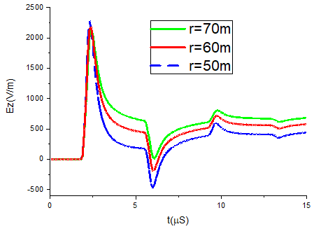
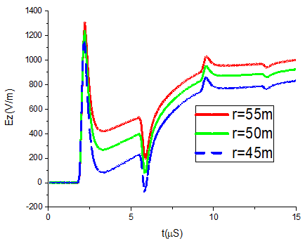
The electric field exhibits a positive shape at 55m from the elevated object (Figure 10), this result is in concordance with those obtained by Eq. (17), although it stills bipolar at the same position for a conducting soil (see Figure 11), the susceptibility behavior field to the ground conductivity is visible, the positive sign locations are resumed in Table 5.
Figure 10. Field waveform sensibility to the ground conductivity (σ=∞)
Figure 11. Field waveform sensitivity to the ground conductivity (σ=0.001S/m)
Table 5. Horizontal distance corresponding to the field transition susceptibility to the ground conductivity change
|
σ (S/m) |
∞ |
0.01 |
0.001 |
|
rcd (m) |
55 |
60 |
70 |
4.5 Variation of the return stroke speed
Figure 12. Field behavior Transients sign (v=1×10⁸ m/S)
Figure 13. Return stroke speed effect on the vertical electric field waveshape (v=2×10⁸ m/S)
In this section, we will variate the return stroke speed in our computation (see Table 6), according to the lightning speed measurements [35], Then we will focus our remarks on the reversed waveshape sign of the electric-field. The CN tower parameters are taken according to the Table 1, the ground conductivity is set as 0.01 S/m.
It’s appears from the Figure 12, that the field tail has risen at the simulation end compared with the wave-shape in Figure 3 and 13. Moreover, the field shape has changed significantly according to the speed set as v=2×10⁸ m/S (Figure 13).
The average polarity reversed localization is about 60m.
The speed difference-ratio generated a variation about 5m to 10m for each reversal field location.
Table 6. Radial-direction distance corresponding to the field susceptibility to the return stroke speed variation
|
v (m/S) |
1×10⁸ |
1.5×10⁸ |
2×10⁸ |
|
rcd (m) |
50 |
60 |
65 |
In this work, we have carried out a parametric study with numerical simulation results in order to analyse the parameters having an impact on the behaviour’s polarity of the vertical electric field to the 553-m tower, the 2D-FDTD technique was applied to solve the Maxwell derivatives formulations in the time propagation domain.
The mathematical expression of the electric field in the source region which is related to the lightning current and the ground conductivity, led us to take each parameter that could influence the field behavior reversion.
The resume of the important analysis results is given as follows:
The vertical electric field shape has a positive pic in the beginning of the simulation time, a negative one in the middle and a positive tail at the end.
The transition from a negative waveform to a positive one is observed at different ranges nearby the elevated structure.
The observation points at the r-axe corresponding to the inversion field polarization is: 1-) Susceptible to the tower height variation, 2-) Raised with the increases of the top reflection tower coefficient., 3-) Decreased with the growth of the bottom reflection tower coefficient, 4-) Inversely- proportional to the ground conductivity change, 5- reversely related to the return stroke speed.
The distances calculated for the polarity-transition have an average of 60m with a maximum of 142m and a minimum of 12m.
The results allowed to clearly characterize the lightning electric field and contribute to the characterization of the lightning phenomenon to tall struck object especially with the need of experimental data for close range.
|
E |
Electric field, V.m-1 |
|
H |
Magnetic Field, A.m-1 |
|
I rcd |
Current, A Crucial horizontal distance |
|
Greek symbols |
|
|
σ |
Ground conductivity, Sm-1 |
|
ε |
Dielectric permittivity, Fm-1 |
|
µ |
Magnetic permeability, Hm-1 |
|
ρ |
Reflection tower coefficient |
|
∆r |
Spatial step in r-axe, m |
|
∆z |
Spatial step in r-axe, m |
|
∆t |
Time step, S |
|
Subscripts |
|
|
i |
Spatial increment in the r-direction |
|
j |
Spatial increment in the z-direction |
|
n |
Time increment |
[1] Zhang, Y., Yang, S., Lu, W., Zheng, D., Dong, W., Li, B., Chen, L. (2014). Experiments of artificially triggered lightning and its application in Conghua, Guangdong, China. Atmospheric Research, 135: 330-343. https://doi.org/10.1016/j.atmosres.2013.02.010
[2] Fisher, R.J., Schnetzer, G.H., Thottappillil, R., Rakov, V.A., Uman, M.A., Goldberg, J.D. (1993). Parameters of triggered-lightning flashes in Florida and Alabama. Journal of Geophysical Research: Atmospheres, 98(D12): 22887-22902. https://doi.org/10.1029/93JD02293
[3] Rakov, V.A. (1999). Lightning discharges triggered using rocket-and-wire techniques. In Recent research developments in geophysics, 2: 141-171.
[4] Rakov, V.A. (2001). Transient response of a tall object to lightning. IEEE Transactions on Electromagnetic Compatibility, 43(4): 654-661. https://doi.org/10.1109/15.974646
[5] Rachidi, F., Janischewskyj, W., Hussein, A.M., Nucci, C.A., Guerrieri, S., Kordi, B., Chang, J.S. (2001). Current and electromagnetic field associated with lightning-return strokes to tall towers. IEEE Transactions on Electromagnetic Compatibility, 43(3): 356-367. https://doi.org/10.1109/15.942607
[6] Heidler, F., Wiesinger, J., Zischank, W. (2001). Lightning currents measured at a telecommunication tower from 1992 to 1998. In 14th International Zurich Symposium on Electromagnetic Compatibility, 6.
[7] Visacro, S., Soares Jr, A., Schroeder, M.A.O., Cherchiglia, L.C., de Sousa, V.J. (2004). Statistical analysis of lightning current parameters: Measurements at Morro do Cachimbo Station. Journal of Geophysical Research: Atmospheres, 109(D1). https://doi.org/10.1029/2003JD003662
[8] Narita, T., Yamada, T., Mochizuki, A., Zaima, E., Ishii, M. (2000). Observation of current waveshapes of lightning strokes on transmission towers. IEEE Transactions on Power Delivery, 15(1): 429-435. https://doi.org /10.1109/61.847285
[9] Schulz, W., Diendorfer, G. (2004). Lightning peak currents measured on tall towers and measured with lightning location systems. In 18th Int. Lightning Detection Conference, Helsinki, Finland.
[10] Romero, C., Paolone, M., Rubinstein, M., Rachidi, F., Rubinstein, A., Diendorfer, G., Zweiacker, P. (2012). A system for the measurements of lightning currents at the Säntis Tower. Electric Power Systems Research, 82(1): 34-43. https://doi.org/10.1016/j.epsr.2011. 08 .011
[11] Romero, C., Rachidi, F., Rubinstein, M., Paolone, M., Rakov, V.A., Pavanello, D. (2013). Positive lightning flashes recorded on the Säntis tower from May 2010 to January 2012. Journal of Geophysical Research: Atmospheres, 118(23): 12879-12892. https://doi.org/10.1002/2013JD020242
[12] McEachron, K.B. (1939). Lightning to the empire state building. Journal of the Franklin Institute, 227(2): 149-217. https://doi.org/10.1016/S0016-0032(39)90397-2
[13] Berger, K. (1975). Parameters of lightning flashes. Electra, 41: 23-37.
[14] Hussein, A.M., Janischewskyj, W., Milewski, M., Shostak, V., Chisholm, W., Chang, J.S. (2004). Current waveform parameters of CN tower lightning return strokes. Journal of Electrostatics, 60(2-4): 149-162. https://doi.org/10.1016/j.elstat.2004.01.002
[15] Diendorfer, G., Hadrian, W., Hofbauer, F., Mair, M., Schulz, W. (2002). Evaluation of lightning location data employing measurements of direct strikes to a radio tower. e & i Elektrotechnik und Informationstechnik, 119(12): 422-427. https://doi.org/10.1007/BF 031613 57
[16] Romeo, C., Rachidi, F., Paolone, M., Rubinstein, M. (2013). Statistical distributions of lightning currents associated with upward negative flashes based on the data collected at the Säntis (EMC) tower in 2010 and 2011. IEEE Transactions on Power Delivery, 28(3): 1804-1812. https://doi.org/10.1109/TPWRD.2013.2254727
[17] Araki, S., Nasu, Y., Baba, Y., Rakov, V.A., Saito, M., Miki, T. (2018). 3-D finite difference time domain simulation of lightning strikes to the 634-m Tokyo Skytree. Geophysical Research Letters, 45(17): 9267-9274. https://doi.org /10.1029/2018GL078214
[18] Rachidi, F., Rakov, V.A., Nucci, C.A., Bermudez, J.L. (2002). Effect of vertically extended strike object on the distribution of current along the lightning channel. Journal of Geophysical Research: Atmospheres, 107(D23): ACL16-1-ACL16-6. https://doi.org/10.1029/2002JD002119
[19] Heidler, F.H., Paul, C. (2017). Some return stroke characteristics of negative lightning flashes recorded at the Peissenberg Tower. IEEE Transactions on Electromagnetic Compatibility, 59(5): 1490-1497. https://doi.org/10.1109/TEMC.2017.2688587
[20] Mimouni, A., Mosaddeghi, A., Rachidi, F., Rubinstein, M. (2008). Electromagnetic fields very near to a tall tower struck by lightning: Influence of the ground conductivity. In European Electromagnetics International Symposium EUROEM 2008 (No. CONF).
[21] Mosaddeghi, A., Pavanello, D., Rachidi, F., Rubinstein, M. (2007). On the inversion of polarity of the electric field at very close range from a tower struck by lightning. Journal of Geophysical Research: Atmospheres, 112(D19). https://doi.org/101029/2006JD008350
[22] Uman, M.A., McLain, D.K., Krider, E.P. (1975). The electromagnetic radiation from a finite antenna. American Journal of Physics, 43(1): 33-38. https://doi.org/10.1119/1.10027
[23] Baba, Y., Rakov, V.A. (2005). Lightning electromagnetic environment in the presence of a tall grounded strike object. Journal of Geophysical Research: Atmospheres, 110(D9). https://doi.org/10.1029/2004JD005505
[24] Thottappillil, R., Schoene, J., Uman, M.A. (2001). Return stroke transmission line model for stroke speed near and equal that of light. Geophysical Research Letters, 28(18): 3593-3596. https://doi.org/10.1029/2001GL013029.
[25] Baba, Y., Rakov, V.A. (2008). Influence of strike object grounding on close lightning electric fields. Journal of Geophysical Research: Atmospheres, 113(D12). https://doi.org/10.1029/2008JD009811
[26] Rachidi, F. (2007). Modeling lightning return strokes to tall structures: A review. In Journal of Lightning Research., 1: 16-31.
[27] Shao, X.M., Lay, E., Jacobson, A.R. (2012). On the behavior of return stroke current and the remotely detected electric field change waveform. Journal of Geophysical Research: Atmospheres, 117(D7). https://doi.org/10.1029/2011JD017210
[28] Zhang, Q., He, L., Ji, T., Hou, W. (2014). On the field-to-current conversion factors for lightning strike to tall objects considering the finitely conducting ground. Journal of Geophysical Research: Atmospheres, 119(13): 8189-8200. https://doi.org10.1002/ 2014jd021496
[29] Yee, K. (1966). Numerical solution of initial boundary value problems involving Maxwell's equations in isotropic media. IEEE Transactions on Antennas and Propagation, 14(3): 302-307. https://doi.org/10.1109/TAP.1966.1138693
[30] Mur, G. (1981). Absorbing boundary conditions for the finite-difference approximation of the time-domain electromagnetic-field equations. IEEE transactions on Electromagnetic Compatibility, (4): 377-382. https://doi.org/10.1109/TEMC.1981.303970
[31] Yang, C., Zhou, B. (2004). Calculation methods of electromagnetic fields very close to lightning. IEEE Transactions on Electromagnetic Compatibility, 46(1): 133-141. https://doi.org/10.1109/TEMC.2004.823626
[32] Baba, Y., Rakov, V.A. (2005). On the use of lumped sources in lightning return stroke models. Journal of Geophysical Research: Atmospheres, 110(D3). https://doi.org/10.1029/2004JD005202
[33] Heidler, F. (1985). Analytic lightning current functions for LEMP calculations. In 18th International Conference on Lightning Protection (ICLP), VDE Verlag, Berlin, West Germany, 453: 63-66.
[34] Mimouni, A., Rachidi, F., Azzouz, Z.E. (2007). Electromagnetic environment in the immediate vicinity of a lightning return stroke. Journal of Lightning Research, 2(ARTICLE): 64-75.
[35] Rakov, V.A. (2007). Lightning return stroke speed. J. Lightning Res, 1: 80-89.