Omolayo M. Ikumapayi* | Benjamin I. Attah | Samuel O. Afolabi | Olurotimi M. Adeoti | Ojo P. Bodunde | Stephen A. Akinlabi | Esther T. Akinlabi
© 2020 IIETA. This article is published by IIETA and is licensed under the CC BY 4.0 license (http://creativecommons.org/licenses/by/4.0/).
OPEN ACCESS
This present paper focused on the numerical modelling and simulation of the influence of friction and drawing tension while validating it with experimental results for both symmetric and axisymmetric plane deformations in stranded and unstranded wire drawing of pure aluminium. It must be noted that several methods have been deployed in recent years such as empirical, numerical, mathematical, analytical, as well as experimental in analyzing and optimizing forces and stresses in wire drawing and there are no definite solutions yet in solving the numerical complexities involved as a result of enormous number of factors during the wire drawing operation. On this note, modelling and simulation with different cases had been established. In this study, 9.50 mm was drawn into different diameters having 4.4 mm as entry and 1.7 mm as exit with intermediate sizes. It was established in the study that half conical angle must be kept as moderate as possible, it must not be too high or too low. An increase in reduction ratio (deformation) leads to an increase in tensile strength and that the tensile strength of material during wire during increases with an increase in the frictional coefficient. The fractographical examination revealed that unstranded aluminium drawn wire is more ductile due to the presence of a large network of dimples which are bimodal and equiaxed dominated by a cup and cone structures and this can be attributed to the ductile failure mode. Whereas the stranded aluminium-drawn wire possessed low ductility as revealed in fractography due to the presence of “Rock Candy fracture”.
aluminium, axisymmetric, coefficient of friction, drawing tension, symmetric, wire drawing
Wire drawing phenomenon is a plastic deformation process that has received great attention in manufacturing industries especially electrical and automotive industries since it allows for improvement in the mechanical strength of the wire [1]. Wire drawing process is a cold working process that involves a reduction in the cross-sectional area and elongation in the length, especially in bars, rods or plates via tensional forces. It is usually pulled through a die with a rigid tool having a wear-resistant surface. The cross-section of a long bar/wire is reduced or altered by applying tensile stress in the form of pulling (drawing) through a die called a draw die. To better understand the process, it is vital to understand the difference between drawing and extrusion. Drawing entails pulling material (that is to be altered) through a die, whereas in extrusion material is pushed through the die. Drawing makes use of tensile stress though there is a slight presence of compressive stress which plays a crucial role in the sense that the material is squeezed as it passes through the die opening. As a result of that, the deformation that results in a drawing is occasionally referred to as indirect compression. Wire products are utilized in various applications, such as electrical wiring, wire-cloth, for window screens, telephone and data wire and cables, the fish-hook and needle industries, wiring of machines and structural components, stringed musical and scientific instruments, bolts and rivets, pin and hair-pin making, pegs and nail as well as shafts for power transmission. It must be noted that there are very few industries in which wiring or wire does not enter [2].
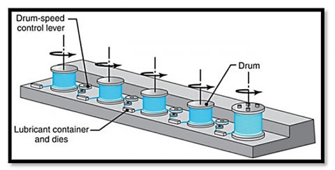
It is essential to note that, we have hydrostatic wire drawing and bundle wire drawing. The former is a type of drawing process that was developed over the years. It is preferably suitable for brittle material as well as composites. The advantage with regards to this drawing process is that it is not compulsory for the stock to be cylindrical or straight and does not require a uniform cross-sectional area along its whole length. Whereas the bundle wire drawing is a type of wire drawing which is mostly popular for increased productivity as many wires are drawn simultaneously as a bundle. This can be advantageous when producing very fine wire, which may be costly. This type of drawing process produces wires that are like a polygonal shape, as opposed to a circular shape in cross-section. When it comes to generating a continuous length, more advanced and sophisticated techniques have been developed to aid in producing fine wire that is chopped into different shapes and sizes. To generate fine wire, a multistage wire drawing must be installed (see Figure 1). For firewire of diameter below 10 mm, this drawing technique is used. The stock is drawn via several dies in series, hence the name multistage wire drawing. Very ductile copper wire is usually a product of such [3].
Figure 1. Multistage wire drawing
Wire drawing is done on a multistage drawing machine that is separated by drums spaced at specific lengths in between the dies. The drums are usually referred to as capstans and of which are motor-driven, providing the pull force needed to draw wire stock. The drums maintain a tolerable tension on the wire as it proceeds to the following die in the series. The total desired reduction is achieved by having the wire pass through the multiple dies, each providing their specific reduction. Multistage wire drawing sometimes requires annealing in between the dies in series. The wire drawing die is usually a conical shape whereby the end of the wire/bar is designed in the form of a point shape which in inserted through the die opening. The stock is prepared first before drawing commences [4]. Work material needs to be ductile as is going to be subjected to tensile forces. Annealing is sometimes applied to provide the necessary ductility if required. For wire drawing operation to be successful the die angle should be taken into great consideration [5]. Due to the drawing processes involving frictional work, which increases with decreasing in die angle, it is therefore important to obtain a precise approach angle that minimizes the friction. It must be noted that a lubricant is usually used to aid in temperature control.
1.1 Lubrication and coefficient of friction
It is crucial to determine the friction conditions in bulk metal forming because of the high contact pressures associated with the process and because friction has an influence on material flow and tool stresses [6]. With the advancement in technology and an increase in demand for cold drawn products, it has become even more important to minimize friction levels during operation. Minimizing friction results in less energy consumption, increased tool life, less production costs, and more productivity. Recent developments have seen the application of Oxalates instead of stainless-steel tubes to minimize friction levels [7]. To maintain a good surface finish and long life of the die used, it is essential that lubrication is applied during the drawing process [8]. There are different means of carrying out a drawing process with or without lubricants. We have the wet drawing in which wire or bar is wholly dipped in a lubricant, we also have the dry drawing in which rod or wire passed through a coated container of lubricant that eventually coated the surface. Similarly, we have a metal coating in which rod or wire are coated with soft metal which served as a solid lubricant and lastly we have ultrasonic vibration in which there is vibration during wire drawing which helps to deduce the forces of friction and hence large reductions take place. The forms of production lubricants are continuously improved and organic oils are being tested as they are preferable" [9]. According to Obi et al. palm oil, groundnut oil, and shear butter oil were all tested as lubricant ingredients not only for wire and bar drawing processes but for extrusion processes [10, 11]. Results from these tests all proved that the type of lubricant used has a significant effect on the amount of force applied in the drawing process. It is pertinent to note that at low die angles, frictional work is predominant in such a situation where surface drag is higher due to larger contact length in approach zone during the deformation process. In order to reduce frictional work, the approach angle must be increased, and this can be achieved by using die surface conditions or lubrication [12]. Coulomb coefficient of friction has been designated to quantify the effect of friction and this is represented by the Greek symbol mu (μ). Practically, the μ varying from 0.01 to 0.07 for non-lubricated (dry) wire drawing and between 0.08 to 0.15 for lubricated (wet) wire drawing [13]. It must be noted that drawing speed is inversely proportional to the coefficient of friction as much as lubrication and surface condition.
1.2 Effect of residual stresses
Residual stresses which are stresses that remain within the material after the product has been manufactured are an important factor to consider when manufacturing through cold drawing operations [14]. These stresses influence the performance of the material in the field and need to be kept as minimal as possible. According to Elices [15], residual stresses that result from cold drawing operations cause creep, fatigue and affect the plastic deformation properties of materials especially in pearlitic materials. As a result of research, there are now methods to manufacture seamless tubes with limited residual stresses after cold drawing. Application of advanced die geometries and performing low-cost treatment operations after cold work also lead to reduced residue stresses [16].
The aim of this study is to understand the effects of friction and tensile loading for symmetric and axisymmetric plane deformations during aluminium (AL1050) wire drawing. This research comprises experimental measurements, analytical methods, modelling and simulation. Aluminium rod, 9.50mm diameter, was cold drawn into various diameters before testing.
2.1 Material
Aluminium rods of series 1xxx at different diameters were used in this research work which were manufactured by Western Rod and wire Limited. The rods were obtained as 9.50 mm from the MicCom Cables and Wires Limited, 3/5 Edun-Alaran Road, Behind Ahmadiya Hospital, Ojokoro, Agege, Lagos. The chemical compositions of the pure aluminium (AL1050) rod in as received form was determined using spark analysis at the quality assurance department of the MicCom Cables and Wires Limited and the obtained result is depicted in Table 1. The properties of the pure aluminium rod (AL1050) used in this research are presented in Table 2.
Table 1. Chemical Analysis of the aluminium (AL1050) rod used in as received form
|
Element |
Al |
Zn |
Fe |
Mn |
Si |
Ti |
Cu |
Mg |
Cr |
|
% Composition |
99.58 |
0.032 |
0.23 |
0.0065 |
0.14 |
0.0075 |
0.0019 |
0.0065 |
0.0009 |
Table 2. Properties of the aluminium (AL1050) rod used in as received form
|
Density, ρ |
2700kg/m3 |
|
Yield stress in simple tension, Y |
21.7×10⁶Pa |
|
Young’s modulus, E |
7×10¹⁰Pa |
|
Plane strain yield stress, S=2K |
1.155Y |
|
Poisson’s ratio, v |
0.33 |
|
Crystal Structure |
Face Centered Cubic |
|
Vickerz Hardness |
167Mpa |
|
Electronegativity |
1.61 (Pauling Scale) |
|
Electrical resistivity |
(20℃) 2.824 nΩ.cm |
|
Melting Point |
660.37℃ (933.52K, 1220.666 0F) |
|
Boiling Point |
2467.0℃ (2740.15K, 4472.6 0F) |
|
Specific Heat |
0.2259 cal/g-k |
|
Density |
@ 293 K: 2.6989 g/cm3 |
|
Atomic Weight |
26.9815386 amu |
|
Ultimate Tensile Strength |
10,000 psi |
|
Bulk Modulus |
76 Gpa |
|
Atomic Radius |
125 pm |
|
Thermal Expansion |
(25℃) 23.1μm/m/k |
|
Thermal conductivity |
(300 k) 2.37 w/m/k |
|
Phase at room temperature |
Solid |
|
Element Classification |
Metal |
|
Colour |
Silver |
2.2 Experimental procedures
In this research work, Tomer drawing Machine was employed in the drawing of the aluminium rod (AL1050) with an original diameter of 9.50 mm and of length 200 mm (20 cm) into different sizes as required. Ten (10) different set of experiment were carried out for both stranded and unstranded aluminium wire rod as reflected in Tables 4 and 5. The rod with initial diameter of 9.50 mm was drawn to various diameter based on the setting of the available die. The experiments were conducted at different conditions having the die semi angle at 6°, coulomb friction coefficient lies within 0 to 0.15 and the half conical angle used was 8°. Similarly, the cross-sectional area reduction lies within 0.2 to 0.97. These parametric values are presented in Table 3.
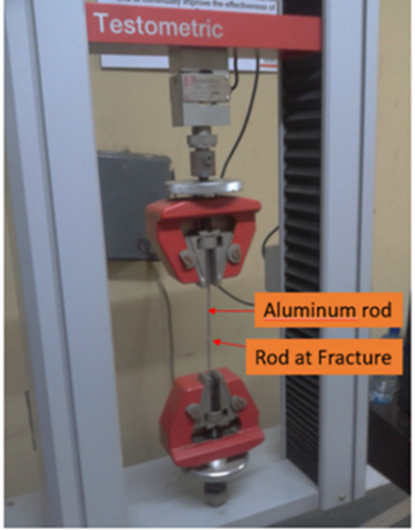
In the same vein, the Testometric materials testing machine (see Figure 2) was used in testing the tensile strength of aluminium wire rod at different diameters and the fractured surfaces were examined under a scanning electron microscope (SEM) to determine the effect of drawing tension on the samples. The Testometric Machine used has a capacity of 100 kN with speed varying from 0.001 to 500 mm/min in steps of 0.001mm/min, Crosshead travel (excluding grips) 1059 mm and Throat 420 mm. The tensile samples were experimented based on the ASTM E8M-13 standard specifications [17]. Both stranded and un-stranded Aluminium (AL1050) wire was tested for tensile strength and a model was developed to validate the experimental results. The tension test has been known as a remarkable tool for determining mechanical properties of materials, like elastic modulus, strength, toughness, strain hardening as well as ductility, hence, the focal point of this research. The drawing parameters used in this research work is presented in Table 3. The test was carried out at ambient temperature until a fracture occurs. Each sample was conducted in triplicate to ensure reproducibility in accordance with the work reported in Srikanth et al. [17].
Table 3. Aluminium wire drawing parametric values
|
Parameters |
Values |
|
Die Semi angle, α (0) |
6 |
|
Coulomb Friction coefficient, μ |
0-0.15 |
|
Cross Sectional area reduction, β |
0.2-0.97 |
|
Half Conical angle, B (0) |
8 |
|
The Problem of Symmetric Plane deformation, n |
1 |
|
The Problem of Axisymmetric Plane deformation, n |
2 |
Figure 2. Tensile sample at fracture
An aluminium wire rod with initial diameter, Do is pulled via a conical die and this propelled plastic deformation of the wire rod, hence, increase in length and decrease in diameter. It is pertinent to note that, frictional force acted between aluminium wire rod and the rough conical die which accelerated the drawing process.
3.1 Model development for numerical analysis
Figure 3 shows a slug representing aluminium rod bonded by the surface of a conical die having two traverse surfaces normal to the axis of symmetry. One is at x distance away from the apex, O whereas the other is at a distance dx with variable incremental of $d \sigma_{x}$. It was assumed during the model that stress $ \sigma_{x}$ is constantly distributed. This is normal to the surface without any shear component. It was also noted that pressure is normal to the surface and that a frictional drag, T is parallel to the surface. During this modelling of tensile stress of wire drawing, the following assumptions were made:
Figure 3. Model representing plastic deformation zone of wire drawing
3.2 Lubrication and coefficient of friction
Let us consider a free-body drawing diagram shown in Figure 4a to predict tensile stress distribution during aluminium wire drawing in a symmetric and axisymmetric conditions, while the free-body diagram to analysis stress state for infinitesimal triangular element is depicted in Figure 4b, when the component of normal pressure of the die is in the x-axis and the free-body diagram required to analysis frictional stress is illustrated in Figure 4c when the component of the frictional stress τ is in the x direction.
Considering the Pressure forces on the die surface,
$\int_{0}^{2 \pi} \operatorname{Ptan} \alpha R(x) d \theta=P \pi R \tan \alpha=P \pi R d R$ (1)
where, α is the angle of the die.
Figure 4. Free-body diagrams for stress analysis (a) Material element; (b) Stress state for infinitesimal triangular Element; (c) Frictional stress for infinitesimal triangular element
Integrate the frictional stress in Eq. (1) along the x-direction,
$\int_{0}^{2 \pi} \mu P d x R(x) d \theta=\frac{\mu P \pi R d x}{2}=\frac{\mu P \pi R d R}{2 \tan \alpha}$ (2)
Taking equilibrium equation along the x- direction for force balancing:
$\left(\sigma_{x}+\frac{d \sigma_{x}}{d x}\right) \frac{\pi[R(x)]^{2}}{4}-\sigma_{x} \frac{\pi R_{0}^{2}}{4}$$-2 P \pi R(x) \frac{d R}{2}-2 \frac{\mu P \pi R d R}{2 \tan \alpha}=0$ (3)
Simplify Eq. (3) by multiplying through by 4 tanα and then collect the common terms:
$\left[\sigma_{x} R^{2}(x)+\frac{d \sigma_{x}}{d x} R^{2}(x)-\sigma_{x} R_{0}^{2}\right] \tan \alpha-$$4 P R(x) \tan \alpha d R-4 \mu P R(x) d R=0$ (4)
It must be noted from Eq. (4) that the shear stress that occurred between the friction of the material and the die is the same to the product of the pressure p and that of the dynamic friction coefficient μ.
Further simplify by dividing each term by:
$R^{2}(x):$$\left[\sigma_{x}+\frac{d \sigma_{x}}{d x}-\sigma_{x}\left(\frac{R_{0}}{R_{x}}\right)^{2}\right] \tan \alpha$$-\frac{4 P}{R(x)}[\tan \alpha+\mu] d R=0$ (5)
Recall that:
$R(x)=R_{0}-x \tan \alpha \Rightarrow\left(\frac{R_{0}}{R_{x}}\right)^{2}=\left(1+\frac{x \tan \alpha}{R(x)}\right)^{2}$ (6)
$=\left(\frac{R_{0}}{R_{x}}\right)^{2}=\left(1-\frac{x d R}{R(x) d x}\right)^{2}$ (7)
Substituting Eq. (7) into Eq. (5) which results to Eq. (8):
$\frac{d \sigma_{x}}{d x}+\frac{n}{R(x)}\left[\sigma_{x} \frac{d R(x)}{d x}-P[\tan \alpha+\mu]\right]=0$ (8)
In this case, n has been generalised and considered for the forces balancing in an equilibrium state.
Taking n equal to 1 for symmetric plane deformation problem, and n equal to 2 for axisymmetric plane deformation problem.
Considering dimensionless values X of position x
$X=\frac{n x t a n \alpha}{R_{o}\left(\frac{A_{0}-A_{1}}{A_{0}}\right)} \Rightarrow x=\frac{X R_{o}\left(\frac{A_{0}-A_{1}}{A_{0}}\right)}{n \tan \alpha} $ (9)
Let the slope between the die contact zone and the material for the conical die be represented by:
$\frac{d R}{d x}=-\tan \alpha \frac{d \sigma_{x}}{d X}+\frac{\left(\frac{A_{0}-A_{1}}{A_{0}}\right)}{\left(1-\frac{x}{R_{0}} \tan \alpha\right) \tan \alpha}$$\left[-\sigma_{x} \tan \alpha-P[\tan \alpha+\mu]\right]=0$ (10)
Put Eq. (9) into Eq. (10), the resulting equation is Eq. (11):
$\frac{d \sigma_{x}}{d X}+\frac{\left(\frac{A_{0}-A_{1}}{A_{0}}\right)}{\left(1-\frac{x\left(\frac{A_{0}-A_{1}}{A_{0}}\right)}{n}\right) \tan \alpha}$$\left[-\sigma_{x}\right.$$ tan \left.\alpha-P[ tan \alpha+\mu]\right]=0$ (11)
For Simplicity, let $\left(\frac{A_{0}-A_{1}}{A_{0}}\right)=\beta$, Eq. (11), therefore gives
$\frac{d \sigma_{x}}{d X}-\frac{\beta}{\left(1-\frac{\beta X}{n}\right) t a n \alpha}$$\left[\sigma_{x} t a n \alpha+P[\tan \alpha+\mu]\right]=0$ (12)
In order to solve Eq. (12) further, there must be a function that connects the pressure P to the drawing Stress.
CASE 1A
Let the linear relationship between P and $\sigma_{x}$ be $P=A-B \sigma_{x} .$ So,
$\frac{d \sigma_{x}}{d X}-\frac{\beta}{\left(1-\frac{\beta X}{n}\right) \tan \alpha}$ (13)
$\left[\sigma_{x} \tan \alpha+\left(A-B \sigma_{x}\right)[\tan \alpha+\mu]\right]=0$
Taking the boundary condition X=0, $\sigma_{x}$=0.
Eq. (13) is of the form:
$\frac{d y}{d x}+P(x)=Q(x)$
$\frac{d \sigma_{x}}{d X}-\frac{\left[\beta \sigma_{x}((1-B) \tan \alpha)-\mu B\right]}{\left(1-\frac{\beta X}{n}\right) \tan \alpha}=\frac{A \beta(\tan \alpha+\mu)}{\left(1-\frac{\beta X}{n}\right) \tan \alpha}$ (14)
$\frac{d \sigma_{x}}{d X}-\frac{[\beta((1-B) \tan \alpha)-\mu B] \sigma_{x}}{\left(1-\frac{\beta X}{n}\right) \tan \alpha}=\frac{A \beta(\tan \alpha+\mu)}{\left(1-\frac{\beta X}{n}\right) \tan \alpha}$
In a simpler form, with the boundary condition X=0, $\sigma_{x}$=0, we have:
Eq. (14) is of the form: $\frac{d y}{d x}+P(x)=Q(x)$, which the integrating factor is $e^{\int P(x) d x}$.
So, Eq. (14) becomes,
$e^{-\int \frac{[\beta(1-B) \tan \alpha-\mu B]}{\tan \alpha\left(1-\frac{\beta}{n} X\right)} \,\,\,\,d X= e^{-\frac{[\beta(1-B) \tan \alpha-\mu B]}{\tan \alpha} \int \frac{d X}{\left(1-\frac{\beta}{n} X\right)}}}$
$=e^{{\frac{n}{\beta}}\left[\frac{\beta(1-B) \tan \alpha-\mu B}{\tan \alpha}\right] \ln \left(1-\frac{\beta}{n} X\right)}$
$=e^{\ln \left(1-\frac{\beta}{n} X\right)^{\frac{n}{\beta}}\left[\frac{\beta(1-B) \tan \alpha-\mu B}{\tan \alpha}\,\,\,\,\,\,\right]}$
$=\left(1-\frac{\beta}{n} X\right)^{\frac{n}{\beta}\left[\frac{\beta(1-B) t a n \alpha-\mu B}{\tan \alpha}\,\,\,\,\,\right]}$ (15)
On multiplying equation,
$\frac{d}{d x}\left[\left(1-\frac{\beta}{n} X\right)^{\frac{n}{\beta}\left[\frac{\beta(1-B) \tan \alpha-\mu B}{\tan \alpha}\right] \sigma_{x}}\right]=\frac{A \beta(\tan \alpha+\mu)}{\left(1-\frac{\beta}{n} X\right) \tan \alpha}$
$\left(1-\frac{\beta}{n} X\right)^{\frac{n}{\beta}\left[\frac{\beta(1-B) \tan \alpha-\mu B}{\tan \alpha}\right] \sigma_{x}}=\int \frac{A \beta(\tan \alpha+\mu)}{\left(1-\frac{\beta}{n} X\right) \tan \alpha} d x$
$\left(1-\frac{\beta}{n} X\right)^{\frac{n}{\beta}\left[\frac{\beta(1-B) t a n \alpha-\mu B}{\tan \alpha}\right] \sigma_{x}}=\frac{A \beta(\tan \alpha+\mu)}{\tan \alpha} \int \frac{d X}{\left(1-\frac{\beta}{n} X\right)}$
$\left(1-\frac{\beta}{n} X\right)^{\frac{n}{\beta}\left[\frac{\beta(1-B) t a n \alpha-\mu B}{\tan \alpha}\right] \sigma_{x}}=-\frac{A \beta(\tan \alpha+\mu)}{\tan \alpha} \cdot \frac{n}{\beta} \ln \left(1-\frac{\beta}{n} X\right)+C$
$\sigma_{x=}-\frac{A \beta(\tan \alpha+\mu)}{\tan \alpha}\left(1-\frac{\beta}{n} X\right)^{-\frac{n}{\beta}\left[\frac{\beta(1-B) t \tan \alpha-\mu B}{\tan \alpha}\right]}+C\left(1-\frac{\beta}{n} X\right)^{-\frac{n}{\beta}\left[\frac{\beta(1-B) \tan \alpha-\mu B}{\tan \alpha}\right]}$
Recall $X=0, \sigma_{x=0}$
$\sigma_{x}=0=-\frac{A \beta(\tan \alpha+\mu)}{\tan \alpha}+C \Rightarrow C=\frac{A \beta(\tan \alpha+\mu)}{\tan \alpha}$
i.e.
$\sigma_{x}=\frac{A \beta(\tan \alpha+\mu)}{\tan \alpha}\left[1-\left(1-\frac{\beta}{n} X\right)^{-\frac{n}{\beta}\left[\frac{\beta(1-B) \tan \alpha-\mu B}{\tan \alpha}\right]}\,\,\,\,\,\,\,\right]$
Therefore,
$\sigma_{x}=\frac{A \beta(\tan \alpha+\mu)}{\tan \alpha}\left[1-\left(1-\frac{\beta}{n} X\right)^{-\frac{n}{\beta}\left[\frac{\beta(1-B) \tan \alpha-\mu B}{\tan \alpha}\right]}\,\,\,\,\,\,\,\right]$ (16)
Therefore, Eq. (16) is the improved model for tensile stress in the wire drawing of pure aluminium.
CASE 1B
Using the classical slab method $P=2 k-\sigma_{x}$
And comparing it with the linear relationship between P and $\sigma_{x}, P=A-B \sigma_{x}$.
Therefore $A=2 k, B=1$.
So, improved tensile stress in Eq. (16) becomes:
$\sigma_{x}=\frac{2 k \beta(\tan \alpha+\mu)}{\tan \alpha}\left[1-\left(1-\frac{\beta}{n} X\right)^{\frac{n}{\beta \tan \alpha}}\right]$
CASE 2
Following Rojas et al. [13], where
$P=\frac{2 k}{1-\tan ^{2}-2 \mu \tan \alpha}-\frac{\left(1-\tan ^{2} \alpha\right) \sigma_{x}}{1-\tan ^{2} \alpha-2 \mu \tan \alpha}$
And comparing it with the linear relationship between P and $\sigma_{x}, P=A-B \sigma_{x}$.
Then
$A=\frac{2 k}{1-\tan ^{2}-2 \mu \tan \alpha}, B=\frac{1-\tan ^{2} \alpha}{1-\tan ^{2} \alpha-2 \mu \tan \alpha}$
Therefore, improved tensile stress in Eq. (16) becomes:
$\sigma_{x}=\frac{2 k \beta(\tan \alpha+\mu)}{\tan \alpha\left[1-\tan ^{2} \alpha-2 \mu \tan \alpha\right]}$$\left[1-\left(1-\frac{\beta}{n} X\right)^{\frac{n}{\beta}\left[\frac{1}{\left(1-\tan ^{2} \alpha-2 \mu \tan \alpha\right) \tan \alpha}\right]\left[\beta \tan ^{2} \alpha+\mu\left(1-\tan ^{2} \alpha\right)\right]}\right]$
Also,
$P=\frac{2 k}{\left[1-\tan ^{2} \alpha-2 \mu \tan \alpha\right]}$$\left[1-\frac{\beta(\tan \alpha+\mu)\left(1-\tan ^{2} \alpha\right)}{\left(1-\tan ^{2} \alpha-2 \mu \tan \alpha\right)}-\right]$
$\frac{2 k \beta(\tan \alpha+\mu)\left(1-\frac{\beta}{n} X\right)^{\frac{n}{\beta}\left[\frac{1}{\left(1-\tan ^{2} \alpha-2 \mu \tan \alpha\right) \tan \alpha}\left[\beta \tan ^{2} \alpha+\mu\left(1-\tan ^{2} \alpha\right)\right]\right]}}{\tan \alpha\left[1-\tan ^{2} \alpha-2 \mu \tan \alpha\right]^{2}}$
CASE 3
We can also use Rojas et al. [13] in which
$P^{i}=\frac{2 k-\left(1-\tan ^{2} \alpha\right) \sigma_{x}^{i}}{1-\tan ^{2} \alpha-2 \mu \tan \alpha+2\left[\left(\frac{P^{i-1}}{2 k}\right) \frac{\tan ^{2} \alpha}{1+\tan ^{2} \alpha}\right]}$
where
$A=\frac{2 k}{\left(1-\tan ^{2} \alpha\right)-2 \mu \tan \alpha+2\left[\left(\frac{P^{i-1}}{2 k}\right) \frac{\tan ^{2} \alpha}{\left(1+\tan ^{2} \alpha\right)}\right]}$
$B=\frac{1-\tan ^{2} \alpha}{\left(1-\tan ^{2} \alpha\right)-2 \mu \tan \alpha+2\left[\left(\frac{P^{i-1}}{2 k}\right) \frac{\tan ^{2} \alpha}{1+\tan ^{2} \alpha}\right]}$
So, improved tensile stress in Eq. (16) becomes
$\sigma_{x}=\frac{2 k \beta(\tan \alpha+\mu)}{\left[\left(1-\tan ^{2} \alpha\right)-2 \mu \tan \alpha+2\left[\left(\frac{P^{i-1}}{2 k}\right) \frac{\tan ^{2} \alpha}{\left(1+\tan ^{2} \alpha\right)}\right]\right] \tan \alpha}$
$\cdot \left[1-\left(1-\frac{\beta}{n} X\right)^{-\frac{n}{\beta}\left[\left[1-\left(\frac{\left(1-\tan ^{2} \alpha\right)}{\left(1-\tan ^{2} \alpha\right)-2 \mu \tan \alpha+2\left[\left(\frac{P^{i-1}}{2 k}\right) \frac{\tan ^{2} \alpha}{\left(1+\tan ^{2} \alpha\right)}\right]}\,\,\,\,\,\,\right)\right]\right]-\frac{\left(1-\tan ^{2} \alpha\right)}{\left[\left(1-\tan ^{2} \alpha\right)-2 \mu \tan \alpha+2\left[\left(\frac{P^{i-1}}{2 k}\right) \frac{\tan ^{2} \alpha}{\left(1+\tan ^{2} \alpha\right)}\right]\right] \tan \alpha}}\,\,\,\,\,\,\,\right]$
The experimental results for both un-stranded and stranded aluminium wire rod (Al 1050) at different diameters are presented in Tables 4 and 5 respectively. The initial diameter of the rod in as received form was 9.50 mm (9.50x10⁻³m). The initial diameter 9.50 mm was then reduced step by step till 1.70 mm while 4.40 mm happened to be the highest reduction, whereas 2.10 mm, 2.50 mm, 2.65 mm, 3.10 mm, 3.25 mm, 3.40 mm, 3.78 mm as well as 4.00 mm were the diameters drawn, based on the available and standard conical die in the company. During the tensile testing, testometric machine recorded breaking force (N) at a peak as well as elongation and this was taking in triplicate to ensure consistency. Then the force means value Fm of the three forces (F1, F2 & F3) was taken and recorded and this was later used to compute the stress.
Table 4. Experimental values for un-stranded wire drawing D0=9.50 mm = 9.50 × 10⁻³ m, $\beta=8^{0}, 2 \alpha=12^{0}, \alpha=6^{0}$
|
S/N |
Di (mm) |
F1 (N) |
F2 (N) |
F3 (N) |
Fm (N) |
A (m2) 10-6 |
$\sigma=\frac{F}{A}\left(\frac{N}{m^{2}}\right)$ |
$\frac{D_{i}}{D_{0}}$ |
$1-\frac{D_{i}^{2}}{D_{0}^{2}}$ |
|
1 |
1.70 |
427.70 |
430.50 |
425.40 |
427.90 |
2.27 |
188.50 |
0.1789 |
0.9680 |
|
2 |
2.10 |
624.40 |
628.30 |
626.80 |
626.50 |
3.46 |
181.07 |
0.2211 |
0.9511 |
|
3 |
2.50 |
862.50 |
865.10 |
864.70 |
864.10 |
4.91 |
176.11 |
0.2632 |
0.9310 |
|
4 |
2.65 |
967.20 |
950.80 |
960.60 |
959.50 |
5.52 |
173.82 |
0.2789 |
0.9222 |
|
5 |
3.10 |
1250.30 |
1265.40 |
1260.60 |
1258.80 |
7.55 |
166.73 |
0.3263 |
0.8940 |
|
6 |
3.25 |
1370.70 |
1374.60 |
1367.30 |
1370.90 |
8.30 |
165.17 |
0.3421 |
0.8830 |
|
7 |
3.40 |
1496.00 |
1490.00 |
1502.00 |
1496.00 |
9.08 |
164.00 |
0.3579 |
0.8720 |
|
8 |
3.78 |
1800.00 |
1830.00 |
1830.00 |
1820.00 |
11.22 |
162.20 |
0.3979 |
0.8417 |
|
9 |
4.00 |
2035.00 |
2030.00 |
2025.00 |
2030.00 |
12.57 |
161.50 |
0.4211 |
0.8227 |
|
10 |
4.40 |
2433.60 |
2435.50 |
2431.70 |
2433.60 |
15.21 |
160.00 |
0.4632 |
0.7855 |
Table 5. Experimental values for stranded wire drawing D0 = 9.50mm = 9.50 ×10⁻³m, $\beta=8^{0}, 2 \alpha=12^{0}, \alpha=6^{0}$
|
S/N |
Di (mm) |
F1 (N) |
F2 (N) |
F3 (N) |
Fm (N) |
A (m2) 10-6 |
$\sigma=\frac{F}{A}\left(\frac{N}{m^{2}}\right)$ |
$\frac{D_{i}}{D_{0}}$ |
$1-\frac{D_{i}^{2}}{D_{0}^{2}}$ |
|
1 |
1.70 |
405.40 |
403.70 |
400.80 |
403.30 |
2.27 |
177.66 |
0.1789 |
0.9680 |
|
2 |
2.10 |
591.80 |
590.10 |
599.30 |
593.73 |
3.46 |
171.60 |
0.2211 |
0.9511 |
|
3 |
2.50 |
820.20 |
825.60 |
822.70 |
822.82 |
4.91 |
167.60 |
0.2632 |
0.9310 |
|
4 |
2.65 |
914.10 |
917.80 |
915.20 |
915.70 |
5.52 |
165.90 |
0.2789 |
0.9222 |
|
5 |
3.10 |
1178.50 |
1180.60 |
1172.20 |
1177.20 |
7.55 |
155.92 |
0.3263 |
0.8940 |
|
6 |
3.25 |
1300.20 |
1290.40 |
1280.10 |
1290.23 |
8.30 |
155.43 |
0.3421 |
0.8830 |
|
7 |
3.40 |
1400.40 |
1390.90 |
1410.00 |
1400.43 |
9.08 |
154.23 |
0.3579 |
0.8720 |
|
8 |
3.78 |
1705.80 |
1710.80 |
1715.70 |
1710.77 |
11.22 |
152.45 |
0.3979 |
0.8417 |
|
9 |
4.00 |
1880.70 |
1880.20 |
1890.50 |
1883.00 |
12.57 |
150.00 |
0.4211 |
0.8227 |
|
10 |
4.40 |
2269.60 |
2270.50 |
2260.70 |
2266.93 |
15.21 |
149.04 |
0.4632 |
0.7855 |
4.1 Effects of frictional coefficient on tensile strength
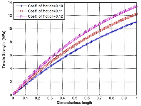
It was assumed in the model that for symmetric plane deformation the value of n is equal to 1. On this basis, for a reduction of 0.2 and the value of the coefficient of friction, μ, values to be 0.1, 0.11 as well as 0.12, the plot is depicted in Figure 5. It was established from the plot that the more the frictional coefficient, the more tensile stress and vice versa for symmetric plane deformation. It was revealed when the coefficient of friction, μ was 0.1, the value of tensile stress was 11 MPa. When the coefficient of friction, μ was 0.11 the tensile stress was 12.2 MPa and lastly when the coefficient of friction, μ was at 0.12, the tensile stress was recorded to be 13.8 MPa. It can be deduced from the above that frictional coefficient must be lower to have a minimum tensile stress and these findings is consistent with the works of Rojas et al. [13] and Rubio et al. [18] where they established the value of coefficient of friction to be between 0.10 and 0.20.
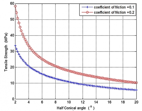
The influence of half conical angle at varying frictional coefficients of 0.1 and 0.2 on tensile strength is presented in Figure 6. It was established from the graph that the frictional coefficient influenced the tensile strength in the wire during operation in correlation with semi conical angle. The graph revealed that the more the frictional coefficient, the more tensile strength and it was also noted that the reduction in semi-conical angle leads to an increase in tensile strength in wire drawing operation. Therefore, it can be deduced that the frictional coefficient is proportional to tensile strength and that tensile strength is inversely proportional to semi conical angle. This assertion agrees with the works of Rojas et al. [13] and Rubio et al. [18].
Figure 5. Plot of tensile strength against dimensionless length
The role of half conical angle during wire drawing operation for symmetric and axisymmetric plane deformation on the tensile strength is presented in Figure 7. It was noted from the graph that when half the conical angle reduces, tensile stress tends to increase for both symmetric and axisymmetric plane deformation. It was established from the graph that the optimal semi-conical angle was 6° and an increase in semi conical angles make the symmetric and axisymmetric plane deformation to be part against each other. This means that there must be moderate value for semi-conical angle, i.e. it must not be too large or too small. This assertion was also in line with the works of Rojas et al. [13] and the work of Rubio et al. [18]. In furtherance to this, Avitzur et al. [19] established that semi-conical angle must be between 3.5° and 14° in order to have minimal drawing tension. The study of Rubio et al. [18] suggested that semi-conical angle should be between 8° – 14° and this present study predicted the value of semi conical angles to be between 8° to 18°.
Figure 6. Plot of Tensile Strength against Half Conical angle at different frictional coefficient
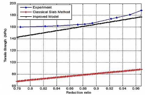
The plot of the experimental result and the results of the simulated model are represented in Figure 8. The result derived from the experiment is being compared with the model results both improved model and that from a classical slab. It was established that there is a close agreement between the improved model and the experimental results as both follow the same trends in a close range and this has validated the simulation of the improved model for tensile strength in wire drawing of aluminium alloy whereas there is a wide range when compared with the simulation form classical slab. It can be deduced that the simulation of the improved model is far better than that of classical slab simulation since there were close values of the experimental and the improved model, and this closeness is also in agreement with the work reported in by Rojas et al. [13] and Rubio et al. [18].
Figure 7. Plot of tensile strength against half conical angle for symmetric and axisymmetric plane deformation
Figure 8. Plot for Experimental result and model simulation
Figure 9. Tensile strength for stranded and unstranded drawn wire
It was revealed in Tables 4 and 5 that unstranded drawn aluminium wires require more breaking forces to fracture than stranded drawn aluminium wires and this was also manifested in their tensile strength as seen in Figure 9. The tables (4 and 5) established that at the entry of the drawn aluminium wire of 4.4 mm, it was note that the tensile strength was 149.04 N/m2 with average breaking force of 2266.93 N in stranded aluminium wire while 160.00 N/m2 and average breaking force of 2433.60 N was produced in unstranded wire. At the exit of 1.7 mm diameter, the stranded wire generated 177.66 N/m2 tensile strength with average breaking force of 403.30 N whereas, the unstranded wire generated 188.50 N/m2 with an average breaking force of 427.90 N. It was further established that increase in the diameters of drawn aluminium wires, require higher forces to fracture and these produced larger amounts of tensile strengths.
4.2 Fractography at the entry and exit
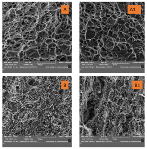
To further determine whether the stranded and unstranded drawn wire is ductile or brittle, fractographical examination was conducted. The fracture surfaces at the entry (4.4 mm) and exit (1.7 mm) for both stranded and unstranded drawn aluminium wire were examined via scanning electron microscope (SEM) and the outcome is presented in Figure 10. The fracture surfaces at the entry and exit for both the stranded and unstranded drawn wire were taking using SEM at 1000x magnification resulting in 50 µm. It was revealed from the morphological examination that unstranded drawn wire was ductile since the microstructure of the fracture surface established several networks of dimples which are bimodal and equiaxed dominated by cup and cone structures and this can be attributed to the ductile failure mode. This ductility property for this type of failure can be attributed to enormous plastic deformation caused by a large force. While for the stranded drawn wire at both entry and exit was seen to have low ductility and this was established because of the formation of “Rock Candy fracture” on both microstructures at entry and exit and this must have caused by sudden loading.
Figure 10. Fracture Surfaces for Unstranded at (A) entry (A1) Exit; for Stranded (B) entry (B1) exit
Wire drawing operation has been studied experimentally and numerically in this research work and the influence of the coefficient of friction and drawing tension for symmetric and axisymmetric plane deformations were established. An improved model was simulated and was used to validate the experimental results. From the research carried out, the results and the discussions, it can be concluded that:
(1) The tensile strength of material during wire during increases with an increase in the frictional coefficient.
(2) The conical angle must be kept at an optimum angle to obtain moderate tensile stress for both symmetric and axisymmetric plane deformations. The half conical angle must not be too small or too large for optimum results.
(3) An increase in reduction ratio (deformation) leads to an increase in tensile strength.
(4) The fractographical examination revealed that unstranded aluminium drawn wire is more ductile due to the presence of a large network of dimples which are bimodal and equiaxed dominated by a cup and cone structures and this can be attributed to the ductile failure mode. Whereas the stranded aluminium-drawn wire possessed low ductility as revealed in fractography due to the presence of “Rock Candy fracture” which showed that the material has low ductile property.
From the work carried out, the results presented, the discussions, and conclusions, it is hereby recommended that:
(1) More Process Parameters such as (Speed, time, coefficient of friction) should be employed and the scope should cover up to five different materials on wire drawing (i.e. Copper, Ferrous, Magnesium alloys, Aluminium Alloys, Gold, Silver etc.).
(2) Further work should be done on this work to cover fatigue, torsion, and impact behavior in order to have a more comprehensive understanding of the metallurgical and mechanical activities that are affected by drawing of aluminium.
The authors would like to thank the Management of MicCom Cables and Wires Ltd, Ojokoro, Agege Lagos for the permission to use their Lab for the research work. We are grateful to the following people for their technical support; Mr Adedipesoye Samson O (Factory Manager), and Mr. Sharma Umankant (Quality Control Technician) of the MicCom Cables and Wires Limited. The Authors are also grateful for the financial support of Pan African University for Life and Earth Sciences Institute (PAULESI), Ibadan, Nigeria for the payment of article publication charges (APC).
|
Parameter |
Unit |
|
P Pressure |
(MPa) |
|
α Die Angle |
(degree, °) |
|
μ Dynamic Friction Coefficient |
(No Unit) |
|
β Area Reduction Ratio |
(No Unit) |
|
S Yield Limit for Tension |
(MPa) |
|
K Yield Shear Stress |
(MPa) |
|
x Die Length |
(mm) |
|
X Dimensional Position |
(mm) |
|
A0 Initial Area |
(mm2) |
|
A1 Final Area |
(mm2) |
|
$\sigma_{0}$ Yield Stress |
(MPa) |
|
Hc Bearing Length |
(mm) |
|
B Reduction Semi-Angle |
(rad) |
|
2B Cone Angle (Reduction Angle) |
(rad) |
|
R0 Initial Radius of the Material |
(mm) |
[1] Filice, L., Ambrogio, G., Guerriero, F. (2013). A multi-objective approach for wire-drawing process. Procedia Cirp, 12: 294-299. https://doi.org/10.1016/j.procir.2013.09.051
[2] Ikumapayi, O.M., Ojolo, S.J., Afolalu, S.A. (2015). Experimental and theoretical investigation of tensile stress distribution during aluminium wire drawing. European Scientific Journal, 11(18): 86-102.
[3] Volkov, A.V., Sokolova, I.D., Korzhavyi, A.P., Beckel, L.S. (2019). Simulation of a copper micro-wire drawing for electronics. IOP Conference Series: Materials Science and Engineering, 537(3): 032054. https://doi.org/10.1088/1757-899X/537/3/032054
[4] Ikumapayi, O.M., Akinlabi, E.T., Onu, P., Abolusoro, O.P. (2020). Rolling operation in metal forming: Process and principles - A brief study. Materials Today: Proceedings, 26: 1644-1649. https://doi.org/10.1016/j.matpr.2020.02.343
[5] Ma, Y.Q., Wu, Y.Z., Gao, H.T., Zhang, Y., Liu, S.Y. (2007). Microstructure and mechanical properties of copper clad aluminium wire by drawing at room temperature. Key Engineering Materials, 334: 317-320. https://doi.org/10.4028/www.scientific.net/KEM.334-335.317
[6] Mohammed, R.J., Ali, J.K., Nassar, A.A. (2019). Numerical analysis of continuous dieless wire drawing process. International Journal of Engineering & Technology, 8: 248-256. https://doi.org/10.14419/ijet.v7i4.19.27986
[7] Tittel, V., Zelenay, M., Kudelas, L. (2012). Effect of drawing angle size of a die on wire drawing and bunching process. Mater. Met.
[8] Saied, E.K., Elzeiny, N.I., Elmetwally, H.T., Abd-Eltwab, A.A. (2020). An experimental study of lubricant effect on wire drawing process. International Journal of Advanced Science and Technology, 29(1): 560-568.
[9] Santana Martinez, G.A., Qian, W.L., Kabayama, L.K., Prisco, U. (2020). Effect of process parameters in copper-wire drawing. Metals, 10(1): 105. https://doi.org/10.3390/met10010105
[10] Obi, A.I., Oyinlola, A.K. (1996). Frictional characteristics of fatty-based oils in wire drawing. Wear, 194(1-2): 30-37. https://doi.org/10.1016/0043-1648(95)06664-0
[11] Ikumapayi, O.M., Oyinbo, S.T., Bodunde, O.P., Afolalu, S.A., Okokpujie, I.P., Akinlabi, E.T. (2019). The effects of lubricants on temperature distribution of 6063 aluminium alloy during backward cup extrusion process. Journal of Materials Research and Technology, 8(1): 1175-1187. https://doi.org/10.1016/j.jmrt.2018.08.006
[12] Oyinbo, S.T., Ikumapayi, O.M., Jen, T.C., Ismail, S.O. (2020). Experimental and numerical prediction of extrusion load at different lubricating conditions of aluminium 6063 alloy in backward cup extrusion. Engineering Solid Mechanics, 8: 119-130. https://doi.org/10.5267/j.esm.2019.10.003
[13] Rojas, H.A.G., Calvet, J.V., Bubnovich, V.I. (2008). A new analytical solution for prediction of forward tension in the drawing process. Journal of Materials Processing Technology, 198(1-3): 93-98. https://doi.org/10.1016/j.jmatprotec.2007.06.053
[14] Ikumapayi, O.M., Akinlabi, E.T., Majumdar, J.D. (2018). Review on thermal, thermo-mechanical and thermal stress distribution during friction stir welding. International Journal of Mechanical Engineering and Technology, 9(8): 534-548.
[15] Elices, M. (2004). Influence of residual stresses in the performance of cold-drawn pearlitic wires. Journal of Materials Science, 39(12): 3889-3899. https://doi.org/10.1023/B:JMSC.0000031470.31354.b5
[16] Lambrighs, K., Wevers, M., Verlinden, B., Verpoest, I. (2011). A fracture mechanics approach to fatigue of heavily drawn steel wires. Procedia Engineering, 10: 3259-3266. https://doi.org/10.1016/j.proeng.2011.04.538
[17] Srikanth, G.S., Liu, Z., Tan, M.J. (2020). Fractography study of Co-Cr-Ni-Mo alloy fatigue wires drawn with different drawing practices. International Journal of Fatigue, 130: 105277. https://doi.org/10.1016/j.ijfatigue.2019.105277
[18] Rubio, E.M., Camacho, A.M., Sevilla, L., Sebastian, M.A. (2005). Calculation of the forward tension in drawing processes. Journal of Materials Processing Technology, 162: 551-557. https://doi.org/10.1016/j.jmatprotec.2005.02.122
[19] Avitzur, B., Hahn Jr, W.C., Iscovici, S. (1975). Limit analysis of flow through conical converging dies. Journal of the Franklin Institute, 299(5): 339-358. https://doi.org/10.1016/0016-0032(75)90173-8