Abderrazak Benchabane* | Fella Charif
OPEN ACCESS
In this paper we propose a gradient based neural network to compute the p-order AR parameters by solving the Yule-Walker equations. Furthermore, to reduce the size of the neural network, we derive a compact architecture of the discrete time gradient based neural network using the fast Fourier transform. For this purpose, the product of the weights matrix and the inputs vector which constitutes the activation of the neurons is performed efficiently in O(p log p) operations and storage instead of O(p2) in the original discrete time gradient based neural network. Simulation results show that proposed neural network architecture is faster and leads to the same results as the original method which prove the correctness of the proposed scheme.
gradient-based neural networks, toeplitz systems, fast fourier transform, auto regressive model
Spectral estimation has been widely used in many practical applications such as radar, speech and communication, to mention a few [1, 2]. Over the last century, a great effort has been made to develop new techniques for high performance spectral estimation. Broadly, the developed techniques can be classified in two categories: nonparametric and parametric methods. The non-parametric spectral estimation approaches are relatively simple, and easy to compute via the Fast Fourier Transform (FFT) algorithm. However, these methods require the availability of long data records in order to yield the necessary frequency resolution. For the parametric approaches, we first design a model for the process of interest which is described by a small number of parameters. Based on this model, the spectral density estimation of the process can be obtained by substituting the estimated parameters of the model in the expression for the spectral density [1].
These parametric methods have a number of advantages as well as disadvantages over non-parametric methods. One of the advantages is their high resolution capability especially with a small number of data records. Also one of the disadvantages is the difficulty of determining a priori the order of the model for a given signal. In addition to these classical problems, many of the alternative spectral estimation methods require intensive matrix computation which may not be practical for real-time processing [3]. When the order of the system is moderate, the system can be efficiently computed in O(p2) flops using the celebrated Levinson-Durbin algorithm. In many problems of signal processing, the order of the system may be large and solving simultaneously this system becomes a challenge task [1].
Neural networks have been widely investigated in parametric spectral estimation [4, 5]. The major advantage of neural network over other methods resides in their capability to perform more complex calculations in real time due to their parallel-disturbed nature. The neural network consists of a large number of simple devices; each one computes little more than weighted sums. Consequently the complexity of computation can be dramatically reduced and the total computation time is comparable to the response time of a single processor which can be very small [6-8].
As well known, the activation of neural networks is based on the computation of a full matrix by vector multiplication where the matrix contains the connection weights and the vector contains the inputs values. Moreover, for the same connection matrix, the multiplication has to be done at each iteration with a new vector input back-warded from the output. In such cases, one seeks to identify special properties of the connection matrix in order to reduce the complexity computation.
In this paper, we derive a compact implementation of the Discrete time Gradient based Neural Networks (CDGNN) for the Auto Regressive (AR) parameters estimation. In the proposed scheme, the multiplication of the weight matrix by the input vector is performed efficiently in O(p log p) operations using the FFT algorithm instead of O(p2) in the original Discrete time Gradient based Neural Networks DGNN [9, 10].
The paper is organized as follows: Section II states the AR parameters estimation problem. In section III, the dynamics of the DGNN to solve this problem is investigated. In Section IV, we present the implementation of the proposed CDGNN model for AR spectral estimation. Computer simulation results for online spectral estimation based on the DGNN model are presented in section V followed by some concluding remarks.
Consider the parameter estimation problem of the noisy AR signal [1, 4]:
$x(n)=-\sum\limits_{i=1}^{p}{{{a}_{i}}}x(n-i)+e(n)$ (1)
where ai , i=1, ...,p are the unknown AR parameters, $x(n-i)\ ,\ i=1, ...,p$ are the p last data samples; e(n) is a zero mean Gaussian process with variance $\sigma_n^2$. Our objective is to get an optimal estimation of the AR parameters using the noisy observations $x(n)_{n=0}^{N-1}$, where N is the number of data points. The parameters to be estimated are the solution of the Yule-Walker equations given by [1]:
$\left[ \begin{matrix} {{r}_{x}}(1) \\ {{r}_{x}}(2) \\ \vdots \\ {{r}_{x}}(p) \\\end{matrix} \right]=-\left[ \begin{matrix} {{r}_{x}}(0) & {{r}_{x}}(-1) & \cdots & {{r}_{x}}(-p+1) \\ {{r}_{x}}(1) & \ddots & {} & \vdots \\ \vdots & \vdots & \ddots & \vdots \\ {{r}_{x}}(p-1) & \cdots & \cdots & {{r}_{x}}(0) \\\end{matrix} \right]\cdot \left[ \begin{matrix} a{}_{1} \\ {{a}_{2}} \\ \vdots \\ {{a}_{p}} \\\end{matrix} \right]$ (2)
where:
${{r}_{x}}(k)=\left\{ \begin{align} & \frac{1}{N}\sum\limits_{n=0}^{N-1-k}{{{x}^{*}}(n)x(n+k)\quad for\ k=0,1,\ldots ,p} \\ & r_{x}^{*}(-k)\quad \quad \ for\ k=-(p-1),-(p-2),\ldots ,-1 \\ \end{align} \right.$
Let:
${{\mathbf{r}}_{x}}=-{{\left[ {{r}_{x}}(1),{{r}_{x}}(2),\cdots ,{{r}_{x}}(P) \right]}^{T}}$
$\mathbf{a}={{\left[ {{a}_{1}},{{a}_{2}},\cdots ,{{a}_{p}} \right]}^{T}}\ $
${{\mathbf{R}}_{x}}\ =\left[ \begin{matrix} {{r}_{x}}(0) & {{r}_{x}}(-1) & \cdots & {{r}_{x}}(-p+1) \\ {{r}_{x}}(1) & \ddots & {} & \vdots \\ \vdots & \vdots & \ddots & \vdots \\ {{r}_{x}}(p-1) & \cdots & \cdots & {{r}_{x}}(0) \\\end{matrix} \right]$
then the above linear equations can be written:
${{\mathbf{R}}_{x}}\mathbf{a}={{\mathbf{r}}_{x}}$ (3)
The power spectrum estimate of the AR signal is formed as:
$P(f)=\frac{\sigma _{n}^{2}}{{{\left| 1+\sum\nolimits_{k=1}^{p}{{{a}_{i}}{{e}^{-j2\pi \,k\,f}}} \right|}^{2}}}$ (4)
where f is the normalized frequency. The true parameters ai, $\sigma_n^2$ should be replaced by their estimates.
In the following, two kinds of recurrent neural networks for the AR parameters estimation will be presented. The former is based on the gradient-descent method in optimization to minimize a quadratic cost function [9-12]. The last, is a simplified architecture of the discrete time gradient based neural networks.
Conventional gradient-based neural networks (GNN) have been developed and widely investigated for online solution of the linear system [9, 13, 14]. To apply the neural networks, the parameters estimation problem must be transformed to a minimization problem suitable for dynamic neural networks processing [13, 14].
Consider the set of linear equations Rx a-rx=0. The design procedure consists to define a norm-based scalar-valued error function and then exploit the negative of its gradient as the descent direction to minimize this function.
According to Eq. (3), let the scalar-valued norm-based energy function:
$E=\frac{1}{2}\left\| {{\mathbf{R}}_{x}}\mathbf{a}-{{\mathbf{r}}_{x}} \right\|_{2}^{2}$ (5)
with $\left\| \cdot \right\|_{2}^{{}}$ denoting the two-norm of a vector. The minimum point of this cost function is the solution of the above linear system Rx a=rx.
To reach a minimum let us take the negative of the gradient of the energy function
$-\frac{\partial E}{\partial \mathbf{a}}=-{{\mathbf{R}}_{x}}^{\mathbf{T}}\left( {{\mathbf{R}}_{x}}\mathbf{a}-{{\mathbf{r}}_{x}} \right)$ (6)
By using a typical continuous-time adaptation rule, Eq. (6) leads to the following differential equation (linear GNN):
$\mathbf{\dot{a}}(t)=\frac{d\mathbf{a}}{dt}=-\frac{\partial E}{\partial \mathbf{a}}=-\gamma \,{{\mathbf{R}}_{x}}^{\mathbf{T}}\left( {{\mathbf{R}}_{x}}\mathbf{a}(t)-{{\mathbf{r}}_{x}} \right)$ (7)
where γ>0 is a design parameter used to scale the GNN convergence rate, and it should be set as large as hardware permits.
We could obtain the general nonlinear GNN model by using a general nonlinear activation function f(×) as follows [14]:
$\mathbf{\dot{a}}(t)=-\gamma \,{{\mathbf{R}}_{x}}^{\mathbf{T}}f\left( {{\mathbf{R}}_{x}}\mathbf{a}(t)-{{\mathbf{r}}_{x}} \right)$ (8)
The discrete-time model of the GNN can be obtained by the use of the forward-difference rule to compute $\mathbf{\dot{a}}(t)$.
$\mathbf{\dot{a}}(t=kh)\approx (\mathbf{a}((k+1)h)-\mathbf{a}(kh))/h$ (9)
where h>0 and k denote the sampling gap and the iteration index respectively. In general, we have ${{\mathbf{a}}_{k}}=\mathbf{a}(t=kh)$ for presentation convenience. Thus the presented DGNN model (8) could be reformulated as:
${{\mathbf{a}}_{k+1}}={{\mathbf{a}}_{k}}-\tau \,{{\mathbf{R}}_{x}}^{T}f\left( {{\mathbf{R}}_{x}}{{\mathbf{a}}_{k}}-{{\mathbf{r}}_{x}} \right)$ (10)
with $\tau =\gamma h$.
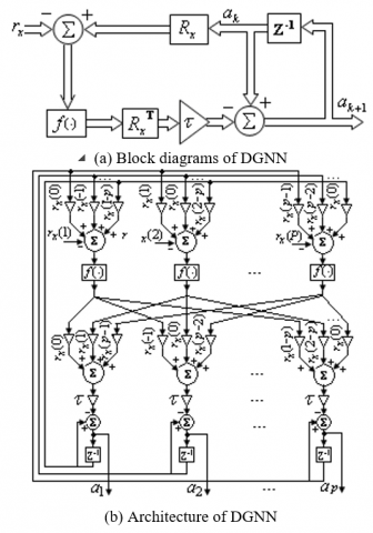
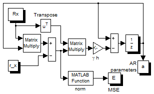
Figure 1. Block diagram and architecture of DGNN
The block diagram realizing and the detailed architecture of the discrete time gradient based neural network are shown in Figure 1. As we can see, we have 2p2 weighting function, p adders of p elements, p adders of p+1 elements and p time-delays.
By setting ${{\mathbf{z}}_{\mathbf{1}}}={{\mathbf{R}}_{x}}{{\mathbf{a}}_{k}}$ , ${{\mathbf{z}}_{2}}=f({{\mathbf{z}}_{1}}-{{\mathbf{r}}_{x}})$and ${{\mathbf{z}}_{3}}=\mathbf{R}_{x}^{T}{{\mathbf{z}}_{2}}$, the dynamic of the neural network can be rewritten in a compact form as:
${{\mathbf{a}}_{k+1}}={{\mathbf{a}}_{k}}-\tau \,{{\mathbf{z}}_{3}}$ (11)
This equation consists of two Toeplitz matrix-vector products ${{\mathbf{z}}_{\mathbf{1}}}={{\mathbf{R}}_{x}}\cdot {{\mathbf{a}}_{k}}$ and ${{\mathbf{z}}_{3}}=\mathbf{R}_{x}^{T}{{\mathbf{z}}_{2}}$ which can be computed efficiently using the algorithm described below.
4.1 Fast matrix-vector product computation
Since Rx is a Toeplitz matrix which is given by its first column and first row, thus it depends only on 2p-1 parameters rather than p2. To compute the product z1=Rxak, the Toeplitz matrix Rx can be first embedded into a circulant matrix $C\in {{\Re }^{2P\times 2P}}$ as follows [15, 16]:
$\boldsymbol{C}=\left[\begin{array}{cc}{\boldsymbol{R}_{x}} & {\boldsymbol{S}} \\ {\boldsymbol{S}} & {\boldsymbol{R}_{x}}\end{array}\right]$ (12)
where
$\mathbf{S}=\left[ \begin{matrix} 0 & {{r}_{x}}(P-1) & {{r}_{x}}(P-2) & \cdots & {{r}_{x}}(1) \\ {{r}_{x}}(1-P) & 0 & {{r}_{x}}(P-1) & \cdots & {{r}_{x}}(2) \\ {{r}_{x}}(2-P) & {{r}_{x}}(1-P) & 0 & \cdots & {{r}_{x}}(3) \\ \cdots & \cdots & \cdots & \cdots & \cdots \\ {{r}_{x}}(-1) & {{r}_{x}}(-2) & {{r}_{x}}(-3) & \cdots & 0 \\\end{matrix} \right]$ (13)
The matrix S never needs to be formed explicitly as C is simply a Toeplitz matrix where the columns are described by the circular-shift of the first column of the matrix C which is of the form:
${{\mathbf{c}}_{1}}=\left[ {{r}_{x}}(0),{{r}_{x}}(1),\cdots , \right.{{\left. {{r}_{x}}(p-1),\ 0\ ,{{r}_{x}}(1-p),{{r}_{x}}(2-p),\cdots ,{{r}_{x}}(p-1) \right]}^{T}}$ (14)
Now we form a new matrix by vector product as follow:
$\mathbf{C}\cdot \left[ \begin{matrix} {{\mathbf{a}}_{k}} \\ {{\mathbf{0}}_{\mathbf{n}}} \\\end{matrix} \right]=\left[ \begin{matrix} {{\mathbf{R}}_{x}} & \mathbf{S} \\ \mathbf{S} & {{\mathbf{R}}_{x}} \\\end{matrix} \right]\cdot \left[ \begin{matrix} {{\mathbf{a}}_{k}} \\ {{\mathbf{0}}_{\mathbf{n}}} \\\end{matrix} \right]=\left[ \begin{matrix} {{\mathbf{R}}_{x}}{{\mathbf{a}}_{k}} \\ \mathbf{S}{{\mathbf{a}}_{k}} \\\end{matrix} \right]$ (15)
Note that the vector ${{[{{\mathbf{a}}_{k}}\ \ {{\mathbf{0}}_{n}}]}^{T}}$is simply the vector ak zero padded to the length of c1 and will be noted $\mathbf{\tilde{a}}$. Then the equation will be rewritten as:
$\mathbf{C}\cdot \mathbf{\tilde{a}}=\left[ \begin{matrix} {{\mathbf{R}}_{\mathbf{x}}}{{\mathbf{a}}_{k}} \\ \mathbf{S}{{\mathbf{a}}_{k}} \\\end{matrix} \right]$ (16)
Then the product ${{\mathbf{R}}_{x}}{{\mathbf{a}}_{k}}$ can be computed efficiently using the following algorithm.
|
Algorithm: Fast matrix-vector product computation |
|
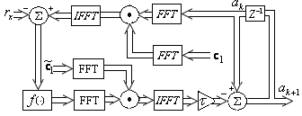
Since the FFT and the IFFT algorithms can be done in $O(p\log p)$ operations, the product ${{\mathbf{R}}_{x}}{{\mathbf{a}}_{k}}$ can be obtained in operations [15, 16]. Figure (2) shows the block diagram illustrating the fast matrix-vector multiplication.
Figure 2. Block diagram illustrating the fast matrix-vector multiplication
4.2 Proposed architecture of CDGNN
To compute the product z3=RxTz2, we do the same steep and we replace Rx by RxT and ak by z2. We note here that RxT is Toeplitz matrix generated by the following vectors [rx (0),rx (-1),⋯,rx (1-p)] and [rx (0),rx (1),⋯,rx (p-1)], and it can be embedded into a circulant matrix CT. The Fourier transform of the first column $\tilde{\boldsymbol{c}}_{1}=\left[r_{x}(0), r_{x}(-1), \cdots, r_{x}(1-p), 0, r_{x}(p-1), r_{x}(p-2), \cdots, r_{x}(0)\right]^{T}$ of the matrix CT will be noted $\boldsymbol{W}$.
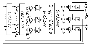
Figure 3. Block diagrams of a simplified DGNN
The block diagram realizing and the detailed architecture of the proposed neural network are shown in the figures (3) and (4) respectively. As we can see, the FFTs of the column c1 and ${{\mathbf{\tilde{c}}}_{1}}$ constitutes the connection weighting of the neural network. So we have just 4p weighting function instead of 2p2 in the original DGNN. The entire circuit contains two blocks FFT/IFFTs, 2 blocks FFT, 2p adders of 2 elements, p time-delays, and 4p weighted connections.
Figure 4. Architecture of the proposed neural network
4.3 Complexity an comparison
As we know, the complexity of a neural network is defined as the total number of multiplications per iteration. It’s well known that the FFT/IFFT using p points require $0.5 p\log p$ multiplications, then it can be seen that the proposed neural network model requires 5p+4p log 2p multiplications per iteration. The original DGNN requires per iteration 2p2+p multiplications. As result, the computational complexity of the proposed neural network is $O(p\log p)$ instead of O(p2) for the DGNN.
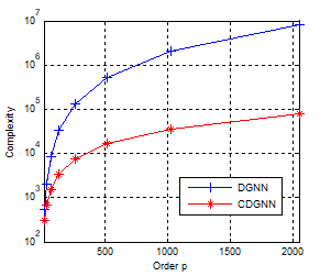
Figure 5. Computational complexity of the two networks
Concerning the memory storage, in addition to $O(p\log p)$ memory required for the FFT/IFFT blocks, we need to store the 6n elements of the vectors c1, ${{\mathbf{\tilde{c}}}_{1}}$, b, and the outputs, thus only $O(p\log p)$ elements need storage in the proposed DGNN instead of O(p2) elements in the original GNN.
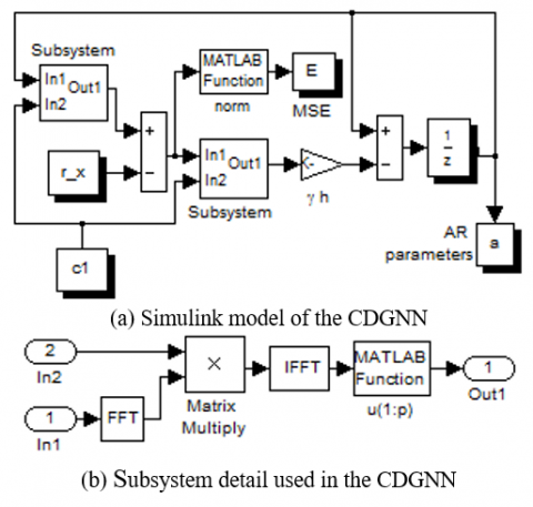
To show the correctness of the proposed neural network architecture and its similarity with the original scheme, the two neural networks have been implemented in the MATLAB Simulink environment on computer with 4 GB RAM and Intel CORE i3 processor with 2.2 GHz. the Simulink implementation of the DGNN and the CDGNN are shown in Figures (6) and (7). The block subsystem which is depicted in Figure (7b) is used to compute z1(kh) and z3(kh) according to the algorithm investigated above.
Figure 6. DGNN MATLAB/Simulink model
Figure 7. CDGNN Simulink model and the subsystems
Computer simulations have been performed to assess the performance of the proposed method in term of accuracy and computational complexity by comparing it with the Yule- Walker method [1].
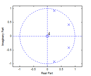
In the firsts experiment, an AR (4) process was generated, with four poles inside the unit circle as shown in Figure 8.
$\begin{align} & x(n)=2.0371x(n-1)-2.4332x(n-2)+ \\ & 1.7832x(n-3)-0.7019x(n-4)+e(n) \\ \end{align}$ (17)
The input e(n) is a white Gaussian process with variance $\sigma_e^2=10^{-2}$.
Figure 8. The pole plot of the AR model (17)
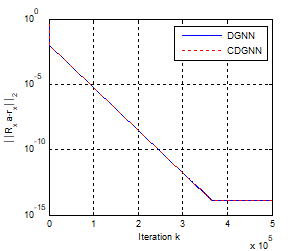
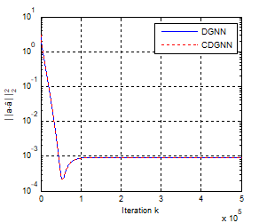
Figure 9. Convergence error of the two neural networks
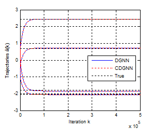
In this example, we let the number of process samples N=64, h=10-4 and γ=55.103. Figures 9, 10 and 11 show the convergence behavior of the original network and its simplified version. As we can see, starting from a random initial state a(0), the two networks converge in the same manner to the true parameters. Figure 9 shows the convergence error of the two networks. It is found that in a few tens of thousands of iterations, the residual error for the two networks is about 10-14. The mean squared error $||\widehat{\boldsymbol{a}}-\boldsymbol{a}\|_{2}^{2}$ after convergence is less than 10-3 for the two networks. This is well illustrated in Figure 10. In Figure 11, we show the trajectories of the estimated parameters.
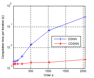
As we can see from this example, both circuits present the same performance. However, the computation time is different. The Figure (12) shows the computation time of both neural networks according to the order of the model. For moderate values of the model order, the computation time of the two networks are similar, however, for large orders, the proposed network is faster. We note here that the computing time is only indicative; it strongly depends on the material used for the simulation.
Figure 10. Mean squared error of the estimated vector parameters
Figure 11. Convergence behaviour of the state trajectory
Figure 12. Computation time of the two networks
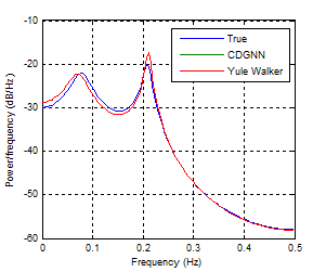
Figure (13) shows the spectral density of the AR (4) process for CDGNN and Yule-Walker methods. The two methods give a similar performance.
Figure 13. Spectral density of the process for different methods
For further illustrative and comparative purposes, let us consider the above model. The simulation results based on 100 realizations are summarized in Table 1. The averaged mean square error (AMSE) is given by:
$A M S E=\frac{1}{M} \sum_{m=1}^{M}\left\|\mathbf{a}-\hat{\mathbf{a}}_{m}\right\|_{2}^{2}$ (18)
where am is the estimated vector using the m-th realization and M the total number of realizations. As we can see from the table, the performances of the Yule-walker method and the proposed simplified neural network are similar.
Table 1. Computed results of estimated parameters using different algorithms
|
|
a1 |
a2 |
a3 |
a4 |
AMSE |
|
True |
-2.0371 |
2.4332 |
-1.7832 |
0.7019 |
0 |
|
Y-W |
-2.0512 |
2.4478 |
-1.8383 |
0.7162 |
0.00091 |
|
CDGNN |
-2.0512 |
2.4478 |
-1.8383 |
0.7162 |
0.00091 |
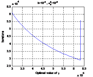
Figure 14. parameter selection
Concerning the selection of the design parameter γ, several simulations were done. As shown in the Figure (14), the optimal value giving a convergence error 10-10 is about 6´105. For smaller values, the convergence time is more important. However for values just greater than the optimum value, the network presents some damped oscillations. If this value is further increased, the network diverges.
We note here, that the optimal value is strongly influenced by the value of the noise variance. For smaller values, a higher value of γ should be used.
Recurrent neural networks are very useful as computational models for solving computationally intensive problems due to their inherent nature of parallel and distributed information processing. The Toeplitz structure of the correlation matrix allows us to design a compact implementation of the gradient based neural network for AR parameters estimation taking the advantage of the fast Fourier transform. The proposed reduced neural network is very suitable for estimating the AR parameters of models with large order. Computer simulations confirm the fastness and the accuracy of the proposed estimator.
[1] Kay SM. (1988). Modern Spectral Estimation: Theory and Application. Englewood Cliffs, NJ: Prentice-Hall.
[2] Zeng X, Shao Z, Lin W, Luo H. (2018). Research on orientation holes positioning of printed board based on LS-power spectrum density algorithm. Traitement du Signal 35(3-4): 277-288. https://doi.org/10.3166/ts.35.277-288
[3] Marple SL. (1987). Digital Spectral Analysis with Applications. Englewood Cliffs, NJ: Prentice-Hall.
[4] Park SK. (1990). Hopfield neural network for AR spectral estimator. In Proc. IEEE, pp. 487-490. http://dx.doi.org/10.1109/ISCAS.1990.112092
[5] Xia Y, Kamel MS. (2006). A cooperative recurrent neural network algorithm for parameter estimation of autoregressive signals. International Joint Conference on Neural Networks, Vancouver, BC, Canada, pp. 2516-2522.
[6] Shao Z, Chen T. (2016). Distributed piecewise H∞ filtering design for large-scale networked nonlinear systems. Eurasip Journal on Advances in Signal Processing 7: 1-12. https://doi.org/10.1186/s13634-016-0350-2
[7] Zhong ZX, Wai RJ, Shao ZH, Xu M. (2017). Reachable set estimation and decentralized controller design for large-scale nonlinear systems with time-varying delay and input constraint. IEEE Transactions on Fuzzy System 25(6): 1629-1643. https://doi.org/10.1109/TFUZZ.2016.2617366
[8] Zhong ZX, Lin CM, Shao ZH, Xu M. (2016) Decentralized event-triggered control for large-scale networked fuzzy systems. IEEE Transactions on Fuzzy System (99): 1-1.
[9] Zhang Y, Chen K, Ma W. (2007). MATLAB simulation and comparison of Zhang neural network and gradient neural network for online solution of linear time-varying equations. International Conference on Life System Modeling and Simulation, Shanghai, China, pp. 450-454.
[10] Stanimirovi´c PS, Petkovi´c MD. (2018). Gradient neural dynamics for solving matrix equations and their applications. Neurocomputing 306: 200-212.
[11] Stanimirovi´c PS, Petkovi´c MD. (2019). Improved GNN models for constant matrix inversion. Neural Process. Lett. https://doi.org/10.1007/s11063-019-10025-9
[12] Shiheng W, Shidong D, Ke W. (2015). Gradient-based neural network for online solution of Lyapunov matrix equation with Li activation function. International Conference on Information Technology and Management Innovation, pp. 955-959. https://doi.org/10.2991/icitmi-15.2015.161
[13] Zhang Y, Chen K. (2008). Global exponential convergence and stability of Wang neural network for solving online linear equations. Electronics Letters 44(2): 145-146. http://dx.doi.org/10.1049/el:20081928
[14] Yi C, Zhang Y. (2008). Analogue recurrent neural network for linear algebraic equation solving. Electronics Letters 44(18): 1078-1079. http://dx.doi.org/10.1049/el:20081390
[15] Pan V. (2001). Structured Matrices and polynomials: Unified Superfast Algorithms. Birkhauser Boston.
[16] Kailath T, Sayed AH. (1999). Fast Reliable Algorithms for Matrices with Structure. SIAM Publications, Philadelphia, PA.