Andres A. Sánchez-Escalona* | Ever Góngora-Leyva | Yanan Camaraza-Medina
OPEN ACCESS
Dimensional analysis was used on this study with the aim of stablishing a model for prediction of the monoethanolamine heat exchangers output. The passive experimentation method was applied to gather 14 400 data points, since the exchangers are installed in an online amine treating unit. After identification of those parameters having a relevant effect on heat transfer processes, the Buckingham Pi theorem and the method of repeating variables were implemented. Once the dimensionless groups were formulated, the explicit equation was found by means of a least-squares regression analysis. The simulation model was evaluated by comparing predicted results against measured rich amine exit temperatures. In this respect, 98.96 % correlation, 0.023 % mean absolute percentage error and 1.376 K maximum absolute error were achieved. Findings of this research may serve as a shortcut for quick and accurate anticipation of the equipment performance, since the plant is often operated outside design parameters. Despite the above, obtained explicit equation is only valid for the studied set of heat exchangers.
amine treatment, CO2 capture, dimensional analysis, heat transfer, industrial applications, performance, prediction
Monoethanolamine (MEA) treating units are common facilities within hydrogen and hydrogen sulphide production plants, and a well-known technology for post combustion carbon dioxide (CO2) capture. Due to actual energy and economic saving needs, these systems improvements became a challenge for engineers and researchers [1-3].
Amine based solutions have the capability of absorbing CO2 when cool (rich amine) and releasing it while heated (lean amine). However, it is a corrosive compound with foaming tendency, which causes noticeable fouling due to heat stable salts formation and deposition. Temperatures beyond 405.15 K triggers amine degradation, which not only leads to acid causing corrosion but also results in decreased CO2 removal efficiency [3]. Under these circumstances, monitoring the heat exchangers outlet temperatures allows process control, fouling rates estimation, and defines fresh MEA make-up needs.
Dimensional analysis has been successfully employed for heat and mass transfer processes study. In this respect, Reynolds ($Re$), Nusselt ($Nu$), Prandtl ($Pr$) among other dimensionless numbers are mandatory references [4-6]. They allow transformation of the system of mass, momentum, energy and species balance equations into non-dimensional forms, thus facilitating generalization of the theoretical and experimental results [7]. Most of the researches aimed to determine empirical heat transfer coefficients are based on this concept [8-14].
Another branch of investigations depending on dimensionless groups is related to basic thermal design theory for recuperators. While the ε-NTU (Effectiveness–Number of Transfer Units) approach is commonly used to determine the heat exchanger outlet temperatures when mass flowrates and inlet temperatures are known, there are other methods like P-NTU (temperature effectiveness), ψ-P (Mueller charts) and P1-P2 (Roetzel–Spang charts) that graphically provides straightforward solutions to the rating and sizing problems [15]. However, calculation of the overall heat transfer coefficient on these procedures is time-consuming and relies on convective heat transfer correlations that are not always accurate.
From consulted literature, only a few researchers focused on simulation of heat exchangers. Laskowski obtained model equations for predicting exit temperatures in two high-pressure regenerators installed in a 200 MW power plant, later proposing simplified and approximated heat transfer effectiveness relations for a steam condenser [16-17]. Although limited to water and steam as working fluids, along with condensed databases (200 data points or less), these publications prove that equipment rating simpler equations can be proposed without including the overall heat transfer coefficient.
Taking the above into consideration, the objective of present research was to establish a model for predicting the rich amine exit temperature in a MEA heat exchangers system, using the Buckingham Pi theorem. The approach shed new light when amine solvents are the process streams, because their thermo-physical properties depends on many variables (temperature, mass fraction, CO2 loading, pressure), are scarce and difficult to estimate.
The remaining part of this paper is organized as follows: Section 2 describes the experimental technique and model deduction methodology, Section 3 provides main modeling results and uncertainty analysis, and Section 4 refers to the conclusions arrived by this study.
2.1 Methodology overview
Dimensional analysis was used for studied heat exchangers modeling. This method facilitates simplification of a given physical phenomenon involving several parameters by rearranging the original set of variables into a reduced number of dimensionless groups. On this context, the Buckingham Pi theorem states that an equation having n number of physical variables which are expressible in terms of j independent fundamental physical quantities, the variables can be grouped in terms of n-j dimensionless parameters called Pi's, related as per Equation (1). The exact form of the function has to be determined on the basis of experimental data [7, 16, 18].
${{\Pi }_{1}}=f({{\Pi }_{2}}\text{, }...\text{, }{{\Pi }_{n-j}})$ (1)
This research first focused on identifying those parameters having a relevant effect on heat transfer processes occurring within the MEA heat exchangers, since omission of an important independent variable yields erroneous results [16]. Thenceforth the experimental method was applied, in order to gather the explanatory variables data sets. Dimensionless groups were formulated later, followed by determination of the model explicit equation by means of a least-squares regression analysis.
Model verification was carried out by comparing predicted results against measured rich amine outlet temperatures [9-10, 16].
2.2 System description and experimental setup
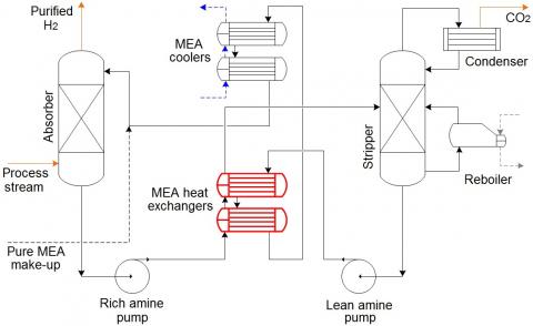
Studied heat exchangers belong to a standard MEA treating unit used for CO2 absorption, installed in a hydrogen production plant (Figure 1).
Figure 1. MEA treating unit diagram
The main process stream enters by the bottom of the absorber, for countercurrent contact with the lean amine flow. During this process CO2 is captured by the solvent, allowing the purified gas to exit the vessel through the top. The rich amine solution, which contains CO2, is then pumped through the MEA heat exchangers in order to raise the temperature above 379 K before getting into the stripper. Within the stripper the amine solution release CO2 for further processing, therefore becoming a lean solvent again. This regenerated amine is pumped back to the absorption column for re-use, initially flowing through the MEA heat exchangers to heat up the rich stream, and further getting across the MEA coolers for lowering the temperature down to 313 K. Pure MEA make-up facilities are used to keep solvent concentration between 12 and 15 % [1, 2].
The MEA heat exchangers system was designed to transfer 2 879 kW of heat, through an area of 180 m2. It consists of two series-installed units, shell-and-tube type, with outer thermal insulation. According to the TEMA standard [19] their designation is “BES”. In each unit the rich amine flows at the tubeside, in two passes, while the lean amine circulates at the shellside, in a single pass. The shell, heads, nozzles and baffles were made from carbon steel, while AISI 316 stainless steel was used for fabrication of the tube bundle.
The passive experimentation method was applied due to the uninterrupted production philosophy of the plant. This procedure consisted of measurement and observation of input and output variables within the normal working regime of investigated heat exchangers, without any manipulation from the researchers, thus analyzing the heat transfer mechanisms as it actually happens [20]. Readings of mass flowrates, inlet and outlet temperatures were performed on each fluid, with the primary instrumentation (Table 1) linked to a Siemens PLC and the SCADA system. A 14 400 data points database was gathered by recording the variables every minute during ten successive days.
Table 1. Primary instrumentation description
|
Parameter |
Instrument description |
Precision |
|
Flow |
Deltabar PMD75 differential pressure transmitter with piezoresistive sensor and welded metallic membrane. |
± 0.05 % |
|
Temperature |
Type K thermocouple with thermowell, wired to TMT-82 Endress+Hauser transmitter. |
± 0.75 % |
2.3 Dimensional analysis
2.3.1 Variables selection
Selection of the model explanatory variables initiated from fundamental heat transfer rate equations applied to heat exchangers: Equation (2), based on first law of thermodynamics; and Equation (3), derived from the ε-NTU method. These equations are valid under no phase change, and assume steady-state, steady flow, plus no heat losses to the surroundings. They also consider that the overall heat transfer coefficient and specific heats are constant throughout the heat exchangers [15].
$Q={{\dot{m}}_{c}}\cdot C{{p}_{c}}\cdot ({{T}_{c,o}}-{{T}_{c,i}})$ (2)
$Q=\varepsilon \cdot min({{\dot{m}}_{c}}\cdot C{{p}_{c}}\text{; }{{\dot{m}}_{h}}\cdot C{{p}_{h}})\cdot ({{T}_{h,i}}-{{T}_{c,i}})$ (3)
where: Q – heat transfer rate, W; $\dot{m}$ – mass flowrate, kg/s; Cp– specific heat at constant pressure, J/(kg·K); T– fluid temperature, K; $\varepsilon $– exchanger heat transfer effectiveness. Subscripts: c– colder fluid (rich amine); h– hotter fluid (lean amine); i– inlet conditions; o– outlet conditions.
Model variables were related by equating the two previous expressions, as stated in Equation (4):
$\begin{align}& {{{\dot{m}}}_{c}}\cdot C{{p}_{c}}\cdot ({{T}_{c,o}}-{{T}_{c,i}})= \\ & \text{ }=\varepsilon \cdot min({{{\dot{m}}}_{c}}\cdot C{{p}_{c}}\text{; }{{{\dot{m}}}_{h}}\cdot C{{p}_{h}})\cdot ({{T}_{h,i}}-{{T}_{c,i}}) \\ \end{align}$ (4)
The exchanger heat transfer effectiveness, defined as the ratio of the actual heat transfer rate to the maximum possible heat exchange rate thermodynamically permitted, can also be written in terms of a few nondimensional parameters as shown in Equation (5) [15, 17]:
$\varepsilon =f(NTU,\text{ }Cr,\text{ flow arrangement})$ (5)
where: NTU– Number of Transfer Units; Cr– heat capacity rate ratio. Equations (6) and (7) were used for their calculation:
$NTU=\frac{U\cdot A}{min({{{\dot{m}}}_{c}}\cdot C{{p}_{c}}\text{; }{{{\dot{m}}}_{h}}\cdot C{{p}_{h}})}$ (6)
$Cr=\frac{min({{{\dot{m}}}_{c}}\cdot C{{p}_{c}}\text{; }{{{\dot{m}}}_{h}}\cdot C{{p}_{h}})}{max({{{\dot{m}}}_{c}}\cdot C{{p}_{c}}\text{; }{{{\dot{m}}}_{h}}\cdot C{{p}_{h}})}$ (7)
where: A– heat transfer surface area, m2; U– overall heat transfer coefficient, W/(m2·K).
Given that the specific heat and other thermo-physical properties of the fluids were assumed as constant, and the overall heat transfer coefficient is a function of both fluids inlet temperatures and mass flowrates [15-16], the dependent and independent variables functional relationship was defined by Equation (8). This equation represents an abbreviated form of Equation (4) for this particular case.
${{T}_{c,o}}-{{T}_{c,i}}=f({{T}_{h,i}}-{{T}_{c,i}}\text{; }{{\dot{m}}_{c}}\text{; }{{\dot{m}}_{h}}\text{; }A)$ (8)
For simplification purposes the above equation was written in terms of the temperature differences, instead of relating each temperature as an independent parameter. It should be noted that, by doing so, primary dimension remains the same.
2.3.2 Dimensionless groups formulation
The method of repeating variables was applied for obtaining the dimensionless groups, whose first step consisted of listing all variables and primary dimensions involved on the analysis (Table 2).
Table 2. Model variables and primary dimensions
|
Variable |
Description |
Dimensions |
|
${{T}_{c,o}}-{{T}_{c,i}}$ |
Rich amine temperature difference |
θ |
|
${{T}_{h,i}}-{{T}_{c,i}}$ |
Maximum temperature difference |
θ |
|
${{\dot{m}}_{c}}$ |
Rich amine mass flowrate |
M1 T-1 |
|
${{\dot{m}}_{h}}$ |
Lean amine mass flowrate |
M1 T-1 |
|
A |
Heat transfer surface area |
L2 |
As observed, five variables (n=5) involving three independent fundamental physical quantities (j=3) were used to describe the heat transfer process occurring within the MEA heat exchangers system. Therefore, two dimensionless groups (n-j=2) were formulated, which are defined by Equation (9) and Equation (10). Selected repeating variables were: maximum temperature difference (${{T}_{h,i}}-{{T}_{c,i}}$); rich amine mass flowrate (${{\dot{m}}_{c}}$); and heat transfer area (A). Their number matches the amount of different primary dimensions.
${{\Pi }_{1}}=({{T}_{c,o}}-{{T}_{c,i}})\cdot {{({{T}_{h,i}}-{{T}_{c,i}}\text{)}}^{{{p}_{1}}}}\cdot {{\text{(}{{\dot{m}}_{c}}\text{)}}^{{{q}_{1}}}}\cdot {{\text{(}A)}^{{{r}_{1}}}}$ (9)
${{\Pi }_{2}}={{\dot{m}}_{h}}\cdot {{({{T}_{h,i}}-{{T}_{c,i}}\text{)}}^{{{p}_{2}}}}\cdot {{\text{(}{{\dot{m}}_{c}}\text{)}}^{{{q}_{2}}}}\cdot {{\text{(}A)}^{{{r}_{2}}}}$ (10)
The terms p, q and r are constant exponents, which were determined by substituting the variables by their dimensions and forcing Pi groups to be dimensionless, as shown in Equations (11) and (12):
$\left\{ {{\text{ }\!\!\theta\!\!\text{ }}^{0}}\text{ }{{\text{M}}^{0}}\text{ }{{\text{T}}^{0}}\text{ }{{\text{L}}^{0}} \right\}=\left\{ {{\text{ }\!\!\theta\!\!\text{ }}^{1}}\cdot {{\text{ }\!\!\theta\!\!\text{ }}^{{{p}_{1}}}}\cdot {{\text{(}{{\text{M}}^{1}}{{\text{T}}^{-1}}\text{)}}^{{{q}_{1}}}}\cdot {{\text{(}{{\text{L}}^{2}})}^{{{r}_{1}}}} \right\}$ (11)
$\left\{ {{\text{ }\!\!\theta\!\!\text{ }}^{0}}\text{ }{{\text{M}}^{0}}\text{ }{{\text{T}}^{0}}\text{ }{{\text{L}}^{0}} \right\}=\left\{ {{\text{(}{{\text{M}}^{1}}{{\text{T}}^{-1}}\text{)}}^{1}}\cdot {{\text{ }\!\!\theta\!\!\text{ }}^{{{p}_{2}}}}\cdot {{\text{(}{{\text{M}}^{1}}{{\text{T}}^{-1}}\text{)}}^{{{q}_{2}}}}\cdot {{\text{(}{{\text{L}}^{2}})}^{{{r}_{2}}}} \right\}$ (12)
Since primary dimensions are by definition independent of each other, the exponents of every primary dimension were individually equated to zero in order to determine the roots (Tables 3 and 4).
Table 3. Exponents calculation for ${{\Pi }_{1}}$
|
Primary dimension |
Equation |
Solution |
|
θ Temperature |
$0=1+{{p}_{1}}$ |
${{p}_{1}}=-1$ |
|
M Mass |
$0={{q}_{1}}$ |
${{q}_{1}}=0$ |
|
T Time |
$0=-{{q}_{1}}$ |
${{q}_{1}}=0$ |
|
L Length |
$0=2{{r}_{1}}$ |
${{r}_{1}}=0$ |
|
Primary dimension |
Equation |
Solution |
|
θ Temperature |
$0={{p}_{2}}$ |
${{p}_{2}}=0$ |
|
M Mass |
$0=1+{{q}_{2}}$ |
${{q}_{2}}=-1$ |
|
T Time |
$0=-1-{{q}_{2}}$ |
${{q}_{2}}=-1$ |
|
L Length |
$0=2{{r}_{2}}$ |
${{r}_{2}}=0$ |
After substitution of calculated exponents into Equation (9) and Equation (10), final expressions of the dimensionless groups were presented. They are defined below by Equations (13) and (14).
${{\Pi }_{1}}=({{T}_{c,o}}-{{T}_{c,i}})\cdot {{({{T}_{h,i}}-{{T}_{c,i}}\text{)}}^{-1}}$ (13)
${{\Pi }_{2}}={{\dot{m}}_{h}}\cdot {{\text{(}{{\dot{m}}_{c}}\text{)}}^{-1}}$ (14)
Lastly, based on the definition given by Equation (1), the function that relates both dimensionless parameters were written. Equation (15) denotes the relationship:
$\frac{{{T}_{c,o}}-{{T}_{c,i}}}{{{T}_{h,i}}-{{T}_{c,i}}}=f\left( \frac{{{{\dot{m}}}_{h}}}{{{{\dot{m}}}_{c}}} \right)$ (15)
3.1 Model explicit equation
The exact function form that correlates the previously-defined dimensionless groups was deduced from a linear regression analysis, hence obtaining Equation (16):
${{\Pi }_{1}}=0,208\cdot {{\Pi }_{2}}+0,4588$ (16)
Then, the model explicit equation was determined by substitution of Equations (13) and (14) into Equation (16) and conveniently rearranging the terms. As a result, Equation (17) was utilized for prediction of the rich amine exit temperature.
${{T}_{c,o}}=\left( 0,208\cdot \frac{{{{\dot{m}}}_{h}}}{{{{\dot{m}}}_{c}}}+0,4588 \right)\cdot ({{T}_{h,i}}-{{T}_{c,i}})+{{T}_{c,i}}$ (17)
It was not necessary to apply dimensional analysis for finding a function to compute the lean amine exit temperature, as it can be determined through an energy balance after calculation of the rich amine outlet temperature, by means of Equation (18):
${{T}_{h,o}}={{T}_{h,i}}-\frac{Q}{{{{\dot{m}}}_{h}}\cdot C{{p}_{h}}}$ (18)
3.2 Modeling results
The predictive ability performance was verified through a scatter plot, by comparing predicted results and measured rich amine exit temperatures (Figure 2). Besides obtaining 98.96 % correlation, computed coefficient of determination informs that 97.93 % of the exit temperature variability was explained by the model.
Figure 2. Model verification
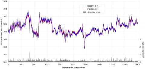
As calculated error indexes (Table 5) are negligible within the studied technological process, proposed approach is considered appropriate for prediction of the MEA heat exchangers output under changed operational conditions of the plant. The satisfactory agreement between results computed form Equation (17) and experimental observations can be corroborated on a trend graph (Figure 3).
Table 5. Prediction errors
|
Criteria |
Absolute error |
Percentage error |
|
Minimum |
0 K |
0 % |
|
Average |
0.088 K |
0.023 % |
|
Maximum |
1.376 K |
0.357 % |
Figure 3. Prediction performance during ten operational days
Achieved accuracy is comparable to the one reported by Laskowski [16], who obtained maximum percentage errors of 0.3 and 0.6 % during prediction of exit temperatures for two high-pressure regenerators installed in a 200 MW power plant by means of the Buckingham Pi theorem.
3.3 Uncertainty analysis
In single-sample experiments, where the variables of interest cannot be repeatedly measured under the same conditions, uncertainty in the results is not obtained by statistical analysis of a series of observations, but evaluated from the systematic errors introduced by direct measurements [21].
In this respect, the experimental setup on this investigation introduced a combined standard uncertainty of 2.223 K when applying the model explicit equation. This value was calculated from Equation (19), which is based on the Law for the Propagation of Uncertainty when input quantities are uncorrelated. It is based on a first-order Taylor series approximation, assuming that errors distribution probability is nearly symmetrical [9,22].
$u_{c}=\left[\left(\frac{\partial \dot{m}_{h}}{\partial T_{c, o}} \cdot u_{\dot{m}_{h}}\right)^{2}+\left(\frac{\partial \dot{m}_{c}}{\partial T_{c, o}} \cdot u_{\dot{m}_{c}}\right)^{2}++\left(\frac{\partial T_{h, i}}{\partial T_{c, o}} u_{T_{h, i}}\right)^{2}+\left(\frac{\partial T_{c, i}}{\partial T_{c, o}} \cdot u_{T_{c, i}}\right)^{2}\right]^{1 / 2}$ (19)
where: ${{u}_{c}}$– combined standard uncertainty; ${{u}_{{{{\dot{m}}}_{c}}}}$, ${{u}_{{{{\dot{m}}}_{h}}}}$, ${{u}_{{{T}_{c,i}}}}$ and ${{u}_{{{T}_{h,i}}}}$– direct measurements uncertainty, usually taken from inaccuracy of the instruments.
It was noticed that the lean amine inlet temperature measurement exerted the greatest influence on the results uncertainty, accounting for its 85.37 %. Therefore, if improved results are required, more accurate instrumentation would have to be installed for measuring this variable.
A model for predicting the rich amine exit temperature in a MEA heat exchangers system was implemented, by applying the Buckingham Pi theorem. This approach avoids calculation of the overall heat transfer coefficient. 98.96 % correlation, 0.023 % mean absolute percentage error and 1.376 K maximum absolute error were achieved when comparing predicted results against the experimental readings.
On this study case obtained explicit equation provides accurate results, and it is easier to apply for determining the fluid outlet temperatures as compared to the ε-NUT method. Major drawback relies on its limited application, as Equation (17) is not recommended for other heat exchanger systems.
The experimental setup introduced a combined standard uncertainty of 2.223 K, being the lean amine inlet temperature measurement of a highest influence. Because no thermo-physical properties are included on the explicit equation, related uncertainty will not affect accuracy of the results.
Considering the advantages of multi-stream equipment over the conventional ones, further studies should focus on extending the approach presented herein to three-fluid heat exchangers modeling. In addition, symbolic regression could be explored to obtain the exact function form that correlates the dimensionless groups.
|
AISI |
American Iron and Steel Institute |
|
ε-NTU |
Effectiveness–Number of Transfer Units |
|
MEA |
Monoethanolamine |
|
PLC |
Programmable Logic Controller |
|
SCADA |
Supervisory Control and Data Acquisition |
|
TEMA |
Tubular Exchanger Manufacturers Association |
|
A |
heat transfer surface area, m2 |
||||
|
Cp |
specific heat at constant pressure, J/(kg·K) |
||||
|
Cr |
heat capacity rate ratio |
||||
|
j |
fundamental physical quantities |
||||
|
$\dot{m}$ |
mass flowrate, kg/s |
||||
|
n |
number of variables |
||||
|
NTU |
Number of Transfer Units |
||||
|
p,q,r |
Dimensional analysis exponents |
||||
|
Q |
heat transfer rate, W |
||||
|
T |
fluid temperature, K |
||||
|
U |
overall heat transfer coefficient, W/(m2·K) |
||||
|
${{u}_{c}}$ |
combined standard uncertainty |
||||
|
${{u}_{{{{\dot{m}}}_{c}}}}$ |
rich amine flowrate measurement uncertainty |
||||
|
${{u}_{{{{\dot{m}}}_{h}}}}$ |
lean amine flowrate measurement uncertainty |
||||
|
${{u}_{{{T}_{c,i}}}}$ |
rich amine inlet temperature measurement uncertainty |
||||
|
${{u}_{{{T}_{h,i}}}}$ |
lean amine inlet temperature measurement uncertainty |
||||
|
Greek symbols |
|
||||
|
$\varepsilon $ |
exchanger heat transfer effectiveness, % |
||||
|
$\Pi $ |
Buckingham Pi dimensionless groups |
||||
|
Subscripts |
|
||||
|
c |
colder fluid (rich amine) |
||||
|
h |
hotter fluid (lean amine) |
||||
|
i |
inlet conditions |
||||
|
o |
outlet conditions |
||||
[1] Aromada SA, Øi LE. (2015). Simulation of improved absorption configurations for CO2 capture. In: Proceedings of the 56th SIMS. Linköping University, Sweden, pp. 21-29. https://doi.org/10.3384/ ecp1511921
[2] Xue B, Yu Y, Chen J, Luo X, Wang M. (2017). A comparative study of MEA and DEA for post-combustion CO2 capture with different process configurations. International Journal of Coal Science & Technology 4(1): 15-24. https://doi.org/10.1007/s40789-016-0149-7
[3] Hajilary N, Nejad AE, Sheikhaei S, Foroughipour H. (2011). Amine gas sweetening system problems arising from amine replacement and solutions to improve system performance. Journal of Petroleum Science and Technology 1(1): 24-30. https://doi.org/10.22078/jpst.2011.15
[4] Jenkins S. (2015). Dimensionless numbers in fluid dynamics. Chemical Engineering 122(2): 38.
[5] Herwig H. (2016). What exactly is the Nusselt number in convective heat transfer problems and are there alternatives? Entropy 18(5): 198. https://doi.org/10.3390/e18050198
[6] Camaraza-Medina Y. (2017). Introducción a la termotransferencia. Editorial Universitaria, La Habana, Cuba.
[7] Yarin LP. (2012). The Pi-theorem Applications to Fluid Mechanics and Heat and Mass Transfer. Springer, New York, USA. https://doi.org/10.1007/978-3-642-19565-5
[8] Tarrad AH, Wahed MA, Khudor DS. (2008). A simplified model for the prediction of the thermal performance for cross flow air cooled heat exchangers with a new air side thermal correlation. Journal of Engineering and Development 12(3): 88-119.
[9] Alshqirate A, Tarawneh M, Mammad M. (2012). Dimensional analysis and empirical correlations for heat transfer and pressure drop in condensation and evaporation processes of flow inside micropipes: Case study with carbon dioxide (CO2). Journal of the Brazilian Society of Mechanical Sciences and Engineering XXXIV(1): 89-96. http://dx.doi.org/10.1590/ S1678-58782012000100012
[10] Muthamizhi K, Kalaichelvi P. (2015). Development of Nusselt number correlation using dimensional analysis for plate heat exchanger with a carboxymethyl cellulose solution. Heat Mass Transfer 51: 815. https://doi.org/10.1007/s00231-014-1455-5
[11] Wami EN, Ibrahim MO. (2014). Model equation for heat transfer coefficient of air in a batch dryer. International Journal of Scientific & Engineering Research 5(11): 121-127.
[12] Dorao CA, Fernandino M. (2017). Dominant dimensionless groups controlling heat transfer coefficient during flow condensation inside pipes. International Journal of Heat and Mass Transfer 112: 465-479. https://doi.org/10.1016/j.ijheatmass transfer.2017.04.104
[13] Medina YC, Khandy NH, Fonticiella OMC, Morales OFG. (2017). Abstract of heat transfer coefficient modelation in single-phase systems inside pipes. Mathematical Modelling of Engineering Problems 4(3): 126-131. https://doi.org/10.18280/ mmep.040303
[14] Camaraza-Medina Y, Hernandez-Guerrero A, Luviano-Ortiz JL, Mortensen-Carlson K, Cruz-Fonticiella OM, García-Morales OF. (2019). New model for heat transfer calculation during film condensation inside pipes. International Journal of Heat and Mass Transfer 128: 344-353. https://doi.org/10.1016/j.ijheatmass transfer.2018.09.012
[15] Shah RK, Sekulić DP. (2003). Fundamentals of Heat Exchangers Design. John Wiley & Sons Inc., New Jersey, USA.
[16] Laskowski RM. (2011). The application of the Buckingham π theorem to modeling high-pressure regenerative heat exchangers in off-design operation. Journal of Power Technologies 91(4): 198-205.
[17] Laskowski RM, Lewandowski J. (2012). Simplified and approximated relations of the heat transfer effectiveness for a steam condenser. Journal of Power Technologies 92(4): 258-265.
[18] Al-Malah KIM. (2017). Exemplification of dimensional analysis via MATLAB® using Eigen values. International Journal of Applied Mathematics and Theoretical Physics 3(1): 14-19. https://doi.org/10.11648/j.ijamtp.20170301.13
[19] Gaddis D. (editor). (2007). Standards of the Tubular Exchanger Manufacturers Association. 9 ed. TEMA Inc., New York, USA.
[20] Hernández-Sampieri R, Fernández-Collado C, Baptista-Lucio MP. (2014). Metodología de la Investigación. 6 ed. McGraw-Hill, Mexico D.F.
[21] Uhia FJ, Campo A, Fernández-Seara J. (2013). Uncertainty analysis for experimental heat transfer data obtained by the Wilson Plot Method. Thermal Science 17(2): 471-487. https://doi.org/10.2298/tsci110701136u
[22] JCGM 100. (2008). Evaluation of measurement data– Guide to the expression of uncertainty in measurement. Centro Español de Metrología, Madrid, Spain.