OPEN ACCESS
Improvement of multifaceted system quality requires a group of complex design modifications. An expanding complexity of system is potentially prone to increase in the failure frequency. Continuous and random occurrence of failures in a system could be the main cause for performance drop of machinery. Theoritical probability distribution is one of the techniques used to estimate the lifetime of a system and its sub-systems with several failure considerations. One of the most extensively used statistical approaches for reliability estimation is a Weibull distribution. In the present paper a three-parameter Weibull distribution approach was adopted to analyze the data sets of Load-Haul-Dumper (LHD) in underground mines using ‘Isograph Reliability Workbench 13.0’ software package. The parameters were evaluated using best fit distributions and Weibull likelihood plots. Percentage reliability of each individual subsystem of LHD was estimated. Further, an attempt has been made to identify the preventive maintenance (PM) time intervals for enhancing the expected rate of reliability.
Weibull distribution, maintenance, reliability, failure rate, LHD
Increase of underground mining activity in India will have obvious positive effects on the demand for mechanized underground mining equipment. Although, the advanced mining technology would find entry into the Indian market, an intermediate level technology comprising LHDs would remain the mainstay of underground coal production, in view of the comparatively smaller size of mines. The average life of LHD could be in between six to ten years [1].
The estimation of equipment life and its possible extension is an important step in the overall decision-making process. Reliability analysis aids in this process to estimate the equipment life. One of the most extensively utilized lifetime distributions for reliability is a Weibull distribution. It is an exceptionally adaptable, suitable distribution for factor estimation and shows the variety sorts of failure rate activities. On the basis of shape parameter, β value, Weibull distribution is a versatile distribution that can take characteristics of other kind of distributions. In a Weibull approximation two or three parameters are utilized for every solution either scale, shape and location parameters. Mixture of strategies is available for assessing the values of these parameters; most of them are analytical and a few are graphical. Graphical strategies incorporate both failure rate (FR) plots and probability density function (PDF) plots. These strategies are not exact but they are moderately quick. The analytical strategies include most extreme probability approaches, the least square strategy and strategy of moments etc. The reliability of a system or sub-system can be estimated using two or three parameter (shape, scale and location) Weibull distributions [2]. Graphical strategies and analytical strategies are very predominant methodologies used for estimating the values of these parameters. Analytical methods like maximum likelihood and least square methods etc., are considered as more accurate strategies. Maximum likelihood method, weighted least, square method and simulation procedures are used to get an exact value [3]. For modeling of best-fit analysis three varieties of Weibull distribution approaches such as 1-parament Weibull, 2-parameter Weibull and 3 parameter Weibull distributions are available. The consequent best-fit data is helpful for the maintenance engineers to make a strategic decision on identification of critical component, that is likely lead to machine failure [4]. In this present analysis a 3-parameter Weibull distribution has been considered to estimate the reliability of sub-systems of LHD.
Reliability estimation is an essential part of mining organization for effective utilization of resources and to improve the health condition of equipment [5]. In order to estimate the Reliability of any kind of system, a wide variety of probability data distribution functions are being used. These could be termed as Exponential function, Lognormal function, Gamma function, 1-Parameter Weibull, 2-Parameter Weibull and 3-Parameter Weibull functions. Among all these methods, Weibull distribution function is one of the most commonly used method to evaluate the reliability [6].
Due to flexibility, the Weibull distribution technique will be broadly utilized to examine the available life data information of the system or sub-system to enhance the desired reliability. Relying upon the values of the parameters, the Weibull distribution could be used to to show an assortment of life behaviors. In this distribution, cumulative probability, failure rate and probability density function (PDF) curves are changed by the influence of either shape paramenter, β, scale parameter, η and location parameter, γ variation. Shape parameter, β, is moreover known as the Weibull slope. Diverse qualities of the shape parameter could need denoted impacts on the behavior of the distribution. In fact, a few values of the shape parameter will cause the distribution equations to decrease. For example, when β = 1, the PDF of 3-parameter Weibull decreases to that of the 2-parameter exponential distribution. The shape parameter β is a dimensionless number.
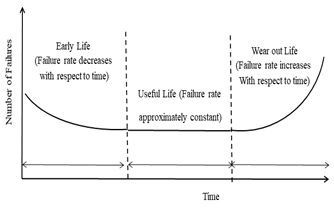
The most imperative perspectives of the shape parameter, β for 3-parameter weibull distributions are: if β < 1 indicates that the rate of failure of a system or component will be decreasing with respect to time, this condition can be treated as early-life failure. Weibull distributions with β nearer to or equivalent to 1 have a constant rate of failure, also known as the useful life zone or arbitrary failure zone. Similarly, Weibull distributions with β > 1 have an increased failure rate with respect to time, denoted as wear-out failure. A typical ‘bathtub curve’ plot clearly depicts the three segments of failure zones. Failure rate of blended Weibull distributions can be possible to observe with β < 1, β = 1 and β > 1 sub-populations. A sample of typical bathtub curve is shown in Fig.1.
Figure 1. Typical bathtub curve (Reference: [8] modified)
3.1 Empirical approximation of Weibull distribution parameters
The empirical approximation of 3-parameter weibull distribution has been derived to identify the relations of PDF, CDF, hazard rate or failure rate and reliability. In order to derive these parameters the unreliability factor can be taken as a linear quadratic model shown in equation (2). This may help to identify the co-ordinates of both x and y-axis to plot the Weibull likelyhood plots. A 3-parameter Weibull distribution’s unreliability or cumulative distribution function (CDF) parameter is shown in equation (1).
$Q(t)=F(t)=1-{{e}^{-{{(\frac{t-\gamma }{\eta })}^{\beta }}}}$ (1)
$Q(t)=1-{{e}^{-{{(\frac{t-\gamma }{\eta })}^{\beta }}}}$
where, ɳ, β & γ are shape, scale and location parameters. The linear form of equation (1) can be written as
$y=mx+c$ (2)
$Q(t)=1-{{e}^{-{{(\frac{t-\gamma }{\eta })}^{\beta }}}}$
$\ln (1-Q(t))=\ln ({{e}^{-{{(\frac{t-\gamma }{\eta })}^{\beta }}}})$
$\ln (1-Q(t))=-{{(\frac{t-\gamma }{\eta })}^{\beta }}$
$\ln (1-Q(t))-\ln (a)=\ln ({{e}^{-{{(\frac{t-\gamma }{\eta })}^{\beta }}}})$
$\ln (-\ln (1-Q(t)))=\beta \ln (\frac{t-\gamma }{\eta })$
$\ln (-\ln (1-Q(t)))=\beta \ln (t-\gamma )-\beta (\eta )$
$\ln (-\ln (\frac{1}{1-Q(t)}))=\beta \ln (t-\gamma )-\beta \ln (\eta )$
$y=\ln (\ln (\frac{1}{1-Q(t)}),x=\ln (t-\gamma )$
Thus the CDF equation can be written as
$y=\beta x-\beta \ln (\eta )$
This is now a linear equation, with an intercept of βln(ɳ) and a slope of β. Co-ordinates of both x and y-axes of the Weibull probability plotting were derived. The x-axis is simply a logarithmic, since x=ln(t-γ). The y-axis is more complex and represented as
$y=\ln (\ln (\frac{a}{Q(t)-1}))$
Reliability is defined as the probability of a machine or its components to perform its designated job over an era of time in acknowledged circumstances. A 3-parameter Weibull distribution’s reliability function is given as
$R(t)={{e}^{-{{(\frac{t-\gamma }{\eta })}^{\beta }}}}$ (3)
The Weibull failure rate function is defined as the quantity of failures per unit time that can be anticipated to happen for the product. It is also known as hazard function, as shown in the equation (4).
$h(t)=\frac{\beta }{\eta }{{(\frac{t-\gamma }{\eta })}^{\beta -1}}$ (4)
The 3-parameter Weibull probability density function f(t) is given as
$PDF=f(t)=\frac{\beta }{\eta }{{(\frac{t-\gamma }{\eta })}^{\beta -1}}{{e}^{-{{(\frac{t-\gamma }{\eta })}^{\beta }}}}$ (5)
$CFD=F(t)=1-{{e}^{-{{(\frac{t-\gamma }{\eta })}^{\beta }}}}$ (6)
The mean time to failure (MTTF) or mean time between failures (MTBF) can be defined as the average life of failure-free operation up to a failure occurrence. The Weibull PDF of MTTF or MTBF is given as
$MTBF=MTTF=\frac{1}{\lambda }$ (7)
where $\lambda =h(t)$ and λ=failure rate
Present case study has been carried out in one of the underground coal mines of the Singareni Collieries Company Limited located in southern region of India. The colliery is currently being operated in Seam 4 and Seam 6 employing the bord and pillar method. Coal extraction is done by drilling and blasting, and LHD is used as the main work horse for coal handling and transportation. LHDs are used to scoop the extracted coal, load it into the bucket, and dump it in the bottom of mine to undergo primary crushing before being hoisted to the surface out of the mine [7]. Fig. 2 shows a typical LHD vehicle performing a loading operation.
Figure 2. A typical LHD machine at working environment
The SCCL operates both underground and open cast mines. 80% of the production comes from opencast mine and 20% is from underground mines. Technology has been a critical factor in the success of SCCL. For open cast mines, it uses technology like shovel dumpers, draglines, in-pit crushing, while for underground mining, it uses technology ranging from (Side-Discharge-Loader) SDLs & LHDs to highly mechanized long wall faces. An increase in productivity and decrease in utilization cost of SCCL can be largely attributed to the phase-wise mechanization and also the adaptation of state-of-the-art technologies.
4.1 Data collection and classification
Before analyzing the machine’s characteristics and failure data, the machine must be classified into a number of systems and subsystems in order to categorize the types of failure occurring on the machine. These classifications will depend up on the maintenance records kept by maintenance personnel, as well as the reasons described by these records, [8]. The classification of subsystems of an LHD are presented in Table 1.
Table 1. Sub-systems classification of LHD
|
Sub-system |
Failure type |
Code |
|
Engine (E) |
Piston-cylinder, radiator |
SSE |
|
Brake (Br) |
Oil leakage, brake jamming |
SSBr |
|
Body (Bo) |
Bucket wear out, welding |
SSBo |
|
Tyre/wheel (Ty) |
Tyre puncher, rim failure |
SSTy |
|
Hydraulic (H) |
Leakages, suspension system |
SSH |
|
Electrical (El) |
Cable reel, socket, sensor |
SSEl |
|
Transmission (Tr) |
Gear train wear out, lubrication |
SSTr |
|
Mechanical (M) |
Structural failure, chassis |
SSM |
|
Machine ID |
Parameter |
SSE |
SSBr |
SSBo |
SSTy |
SSH |
SSEl |
SSTr |
SSM |
|
E1-LHD1 |
FF (%) |
4 |
4 |
6 |
12 |
4 |
16 |
4 |
16 |
|
TBF (Hrs) |
881 |
883 |
576 |
288 |
883 |
211 |
880 |
2012 |
|
|
TTR (Hrs) |
199 |
199 |
133 |
66 |
199 |
50 |
199 |
50 |
|
|
E2-LHD2 |
FF (%) |
6 |
4 |
4 |
7 |
11 |
15 |
5 |
21 |
|
TBF (Hrs) |
644 |
979 |
977 |
558 |
341 |
259 |
785 |
155 |
|
|
TTR (Hrs) |
193 |
289 |
289 |
165 |
105 |
77 |
231 |
56 |
|
|
E3-LHD3 |
FF (%) |
4 |
3 |
3 |
7 |
5 |
18 |
5 |
17 |
|
TBF (Hrs) |
845 |
1129 |
1132 |
478 |
676 |
183 |
676 |
181 |
|
|
TTR (Hrs) |
145 |
194 |
194 |
83 |
116 |
32 |
116 |
34 |
|
|
E5-LHD5 |
FF (%) |
7 |
3 |
6 |
14 |
4 |
18 |
2 |
16 |
|
TBF (Hrs) |
535 |
1254 |
625 |
264 |
940 |
202 |
1879 |
222 |
|
|
TTR (Hrs) |
70 |
164 |
82 |
35 |
123 |
27 |
247 |
31 |
|
|
E6-LHD6 |
FF (%) |
4 |
5 |
5 |
6 |
5 |
20 |
3 |
17 |
|
TBF (Hrs) |
977 |
782 |
782 |
648 |
781 |
188 |
1307 |
215 |
|
|
TTR (Hrs) |
148 |
118 |
118 |
99 |
118 |
30 |
197 |
35 |
|
Machine ID |
Weibull Model |
Weibull Paramete (ɳ=scale/life,β=shape, γ=location) |
||
|
|
|
ɳ |
Β |
Γ |
|
E1-LHD1 |
Weibull 3P |
132.5 |
1.094 |
25.97 |
|
E2-LHD2 |
Weibull 3P |
208.3 |
1.802 |
-4.245 |
|
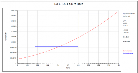
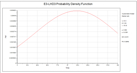
E3-LHD3 |
Weibull 3P |
233.3 |
3.264 |
-93.92 |
|
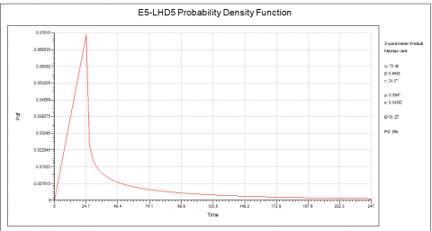
E5-LHD5 |
Weibull 3P |
70.48 |
0.668 |
24.75 |
|
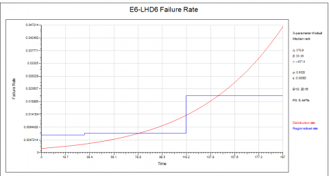
E6-LHD6 |
Weibull 3P |
570.9 |
10.16 |
-437.4 |
Table.4. Failure rate (FR) and probability density function (PDF) of LHDs with reference to each sub-system
|
Machine ID |
Parameter |
SSE |
SSBr |
SSBo |
SSTy |
SSH |
SSE |
SSTr |
SSM |
|
E1-LHD1 |
FR |
0.0039 |
0.0067 |
0.0070 |
0.0074 |
0.0078 |
0.0078 |
0.0081 |
0.0085 |
|
|
0.0038 |
0.0060 |
0.0057 |
0.0050 |
0.0046 |
0.0039 |
0.0035 |
0.0030 |
|
|
TTR (Hrs) |
199 |
199 |
133 |
66 |
199 |
50 |
199 |
50 |
|
|
E2-LHD2 |
FR |
0.0085 |
0.0104 |
0.0104 |
0.0076 |
0.0055 |
0.0044 |
0.0095 |
0.0032 |
|
|
0.0032 |
0.0022 |
0.0022 |
0.0035 |
0.0038 |
0.0035 |
0.0027 |
0.0029 |
|
|
TTR (Hrs) |
193 |
289 |
289 |
165 |
105 |
77 |
231 |
56 |
|
|
E3-LHD3 |
FR |
0.0135 |
0.0225 |
0.0225 |
0.0088 |
0.0110 |
0.0039 |
0.0110 |
0.0039 |
|
|
0.0054 |
0.0030 |
0.0030 |
0.0052 |
0.0054 |
0.0039 |
0.0054 |
0.0033 |
|
|
TTR (Hrs) |
145 |
194 |
194 |
83 |
116 |
32 |
116 |
34 |
|
|
E5-LHD5 |
FR |
0.0106 |
0.0074 |
0.0093 |
0.0134 |
0.0084 |
0.0765 |
0.0064 |
0.0134 |
|
|
0.0048 |
0.0014 |
0.0033 |
0.0081 |
0.0024 |
0.0754 |
0.0007 |
0.0081 |
|
|
TTR (Hrs) |
70 |
164 |
82 |
35 |
123 |
27 |
247 |
31 |
|
|
E6-LHD6 |
FR |
0.0259 |
0.0138 |
0.0138 |
0.0099 |
0.0138 |
0.0023 |
0.0467 |
0.0034 |
|
|
0.0056 |
0.0064 |
0.0064 |
0.0058 |
0.0064 |
0.0020 |
0.0025 |
0.0029 |
|
|
TTR (Hrs) |
148 |
118 |
118 |
99 |
118 |
30 |
197 |
35 |
4.4 Results and discussion.Weibull parameter estimation
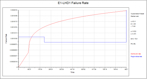
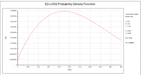
Weibull distribution parameters were estimated using ‘Isograph Reliability Workbench 13.0’ software tool. The statistical values of reliability, unreliability, failure rate, PDF and CDF have been computed accurately by utilizing failure and repair data of each LHD. The estimated data of Weibull parameters are shown in Table 3.
4.5 Estimation of reliability and Un-reliability
The percentage of reliability and unreliability of each individual sub-system of LHDs are determined based on 3-parameter weibull probability distribution function using Isograph reliability workbench 13.0 (Table 5).
|
Machine ID |
Parameter |
SSE |
SSBr |
SSBo |
SSTy |
SSH |
SSEl |
SSTr |
SSM |
|
E1-LHD1 |
F (%) |
55.95 |
67.86 |
44.05 |
32.14 |
79.76 |
8.33 |
91.67 |
20.24 |
|
R (%) |
44.05 |
32.14 |
55.95 |
67.86 |
20.24 |
91.67 |
8.33 |
79.76 |
|
|
TTR (Hrs) |
199 |
199 |
133 |
66 |
199 |
50 |
199 |
50 |
|
|
E2-LHD2 |
F (%) |
55.95 |
79.76 |
91.67 |
44.05 |
32.14 |
20.24 |
67.86 |
8.33 |
|
R (%) |
44.5 |
20.24 |
8.33 |
55.95 |
67.86 |
79.76 |
32.14 |
91.67 |
|
|
TTR (Hrs) |
193 |
289 |
289 |
165 |
105 |
77 |
231 |
56 |
|
|
E3-LHD3 |
F (%) |
67.86 |
79.76 |
91.67 |
32.14 |
44.05 |
8.33 |
55.95 |
20.24 |
|
R (%) |
32.14 |
2024 |
8.33 |
67.86 |
55.95 |
91.67 |
44.05 |
79.76 |
|
|
TTR (Hrs) |
145 |
194 |
194 |
83 |
116 |
32 |
116 |
34 |
|
|
E5-LHD5 |
F (%) |
44.05 |
79.76 |
55.95 |
32.14 |
67.86 |
8.33 |
91.67 |
20.24 |
|
R (%) |
55.95 |
20.24 |
44.05 |
67.86 |
32.14 |
91.67 |
8.33 |
79.76 |
|
|
TTR (Hrs) |
70 |
164 |
82 |
35 |
123 |
27 |
247 |
31 |
|
|
E6-LHD6 |
F (%) |
79.76 |
44.05 |
55.95 |
32.14 |
67.86 |
8.33 |
91.67 |
20.24 |
|
R (%) |
20.24 |
55.95 |
44.05 |
67.86 |
32.14 |
91.67 |
8.33 |
79.33 |
|
|
TTR (Hrs) |
148 |
118 |
118 |
99 |
118 |
30 |
197 |
35 |
PM is defined as the set of activities performed in an attempt to hold the components as per desired condition [11]. In this paper these intervals were computed with respect to the expected percentage of reliability as show in Table 6. From the calculated quantities it is estimated that if the requirement of reliability is 90% for E1-LHD1, then the PM schedule should be conducted at a frequency of every 38 hours. Similarly, for E2-LHD2, E3-LHD3, E5-LHD5 and E6-LHD6 the durations are 56 hours, 23 hours, 27 hours and 20 hours respectively.
Table 6. Reliability based PM time intervals for LHDs
|
Reliability Level |
Preventive Maintenance Time Interval, Hrs |
||||
|
E1-LHD1 |
E2-LHD2 |
E3-LHD3 |
E5-LHD5 |
E6-LHD6 |
|
|
0.90 |
38 |
56 |
23 |
27 |
20 |
|
0.85 |
50 |
72 |
40 |
30 |
40 |
|
0.80 |
62 |
87 |
54 |
32 |
55 |
|
0.75 |
73 |
100 |
65 |
36 |
68 |
|
0.70 |
84 |
114 |
76 |
40 |
79 |
Continuous operation of equipment with a minor failures can only be possible by organizing the proper maintenance planning and implementation. Highest equipment availability and its effective utilization are the two important factors to improve the reliability. Reliability of LHDs was calculated with 3- parameter Weibull distribution analysis. The empirical approximation of this distribution was derived to identify the relations of PDF, CDF, FR and reliability. Weibull distribution parameters such as scale, shape and location parameters were estimated with respect to failure and repair data set. It was observed that the lowest level of reliability was associated with SSEl (8.33%) and SSM (20.24 %) in most of the LHDs (Table 5). It was concluded that unexpected breakdowns and its consequent idle times of the machine are the major causes for reduction in overall equipment performance. Computation of reliability based PM schedules, aids in designing and implementing a maintenance strategy that would potentially increase/enlarge the expected life of the machine. From the results it was observed that in order to achieve the maximum level of reliability i.e., 90%, effective preventive maintenance is necessary for every 38 hrs for E1-LHD1; for E2-LHD2 this could be 56 hours; E3-LHD3 for this could be 23 hours etc (Table 6). In this study overall equipment performance of the LHDs was not considered and performance evaluation was based only on availability and utilization calculations. Future research should include measurement of key performance indicators (KPI).
[1] Balaraju J, Govinda Raj M, Murthy ChSN. (2017). Performance of load haul dumper in underground mines- an overview, proc. of international conference on deep excavation. Energy Resources and Production, IIT, Kharagpur.
[2] Dolas DR, Jaybhaye MD, Deshmukh SD. (2014). Estimation the system reliability using weibull distribution. Proc. of Economics Development and Research 75-79. https://doi.org/10.7763/IPEDR
[3] Bhupesh Kumar L, Makarand S, Kulkarni A. (2010). Parameter estimation method for machine tool reliability analysis using expert judgment. International Journal of Data Analysis Techniques and Strategies 2(2): 155-169. https://doi.org/10.1504/IJDATS.2010.032455
[4] Joselin Herbert GM, Iniyan S, Goic R. (2010). Performance, reliability and failure analysis of wind farm in a developing country. International Journal of Renewable Energy 35: 2739-2751. https://doi.org/10.1016/j.renene.2010.04.023
[5] Harish Kumar NS, Choudhary RP, Murthy ChSN. (2017). Reliability analysis of dumper in lime stone mine based on weibull distribution. Proc. of 91st The IRES International Conference, Chicago, USA.
[6] Ahmad MR, Salih AA, Mahdi AA. (2009). Estimation accuracy of weibull distribution parameters. Journal of Applied Sciences Research 5(7): 790-795.
[7] BalaRaju J; Govinda Raj M, Murthy ChSN. (2017). Improvement of overall equipment effectiveness of load haul dump machines in underground coal mines, world academy of science, engineering and technology. International Science Index, International Journal Materials and Metallurgical Engineering 11(11): 1917.
[8] Vagenas N, Runciman N, Clement SR. (1997). A methodology for maintenance analysis of mining equipment. International Journal of Surface Mining, Reclamation and Environment 11: 33-40. https://doi.org/10.1080/092081197008944053
[9] Oyebisi T. (2000). On reliability and maintenance management of electronic equipment in the tropics. Journal of Underground Resources 20: 517-522. https://mining.archives.pl/2011.04.56
[10] Mohammad Javad R, Seyed Hadi H, Mohammad A, Reza K. (2013). The reliability and maintainability analysis of pneumatic system of rotary drilling machines. The Institution of Engineers (India). https://doi.org/10.1007/s40033-013-0026-0
[11] Bhattacharya P. (2010). A study on weibull distribution for estimating the parameters. Journal of Applied Quantitative Methods 5(2): 234-241. https://doi.org/10.17148/IJREEICE.2017.5308