A. Naamane | M. Hasnaoui
OPEN ACCESS
The object of this paper is the modeling a supersonic flow of inviscid fluid around a dihedral airfoil. Based on the thin airfoils theory and the non-dimensional stationary Steichen equation of a two-dimensional supersonic flow in isentropic evolution, we obtain a solution for the downstream velocity potential of the oblique shock at the second order of relative thickness. This result has been dealt by the asymptotic analysis and characteristics method.
In order to validate our model, the results are discussed in comparison with theoretical and experimental results. Indeed, firstly, the comparison of the results of our model, has shown that they are quantitatively acceptable compared to the existing theoretical results. Finally, an experimental study was conducted using the AF300 supersonic wind tunnel. In this experiment, we have considered the incident upstream Mach number over a symmetrical dihedral airfoil wing. The validation and the accuracy of the results support our model.
asymptotic modeling, characteristics method, weak oblique shock wave, supersonic flow, dihedral airfoil, supersonic wind tunnel
Supersonic flows are frequently encountered in many fields of application. Indeed, many aerospace applications are concerned regular by highly compressible flows (aircraft, spaceship, missile...). In general, all these flows are very complex, despite, for simple geometries involving straight and oblique shocks, detachments and attachments and strong interactions between shock waves and boundary layers. For these studies, several resolutions have been adopted based on numerical simulation or experimental measurements [1-2]. The numerical modeling of supersonic flow around the airfoils has been the topic of wide research, in the engineering applications [3]. The combination of analytical and numerical methods is conceivable by study of chaotic motions [4].
Others studies interested to local existence and the uniqueness of weak shock solution in steady supersonic flow past a wedge [5]. An analytical solution for the generation of shock wave obtained a result of supersonic flow around a wedge [6]. Others methods are deployed to study the supersonic flow profile: the method of hydraulic analog simulation (the method of gas-hydraulic analogy) [7] and simulation using both continuum and particle approaches with inter-molecular collision modeling [8].
In this work, we use asymptotic methods to develop a model of a supersonic flow around thin wing airfoil. Then, we employ an application on the dihedral airfoil and an experimental study to validate the developed model.
For a compressible, isentropic, and irrotational Eulerian fluid flow, and in a two-dimensional steady-state case, the Steichen Equation for the Velocity is, namely:
$\left(u^{* 2}-c^{2}\right) \frac{\partial^{2} u^{*}}{\partial x^{* 2}}+\left(w^{* 2}-c^{2}\right) \frac{\partial^{2} w^{*}}{\partial z^{* 2}}+u^{*} w^{*}\left(\frac{\partial w^{*}}{\partial x^{*}}+\frac{\partial u^{*}}{\partial z^{*}}\right)=0$ (1)
where, u*(x*, z*), w*(x*, z*) are the velocity components (dimensional quantities are characterized by a ∗), and c the speed of sound for the isentropic fluid flow.
At this level, we introduce scaled variables, namely:
$u=\frac{u^{*}}{U_{\infty}} ; w=\frac{w^{*}}{U_{\infty}} ; x=\frac{x^{*}}{L} ; z=\frac{z^{*}}{L}$ (2)
where, U∞ is the uniform constant velocity at upstream infinity; L is the length of the body.
The non-dimensional boundary condition associated to Eq. (1), is the slip-condition, as:
$\vec{u} \cdot \vec{n}=0$ (3)
where, $\vec{n}$ is the unit normal vector to body.
Let us linearize equations (1) about the particular solution, far upstream of an obstacle, as:
$u=1+\varepsilon \frac{\partial \varphi}{\partial x} w=\varepsilon \frac{\partial \varphi}{\partial z}$ (4)
where, φ(x, z) is the velocity potential around the body, and $\varepsilon$ characterizes a perturbation parameter. Thus, taking into account (2) and substituting (4) into (1), we obtain the non-dimensional Steichen Equation, namely:
$\left[M_{\infty}^{2}\left(1+\varepsilon \frac{\partial \varphi}{\partial x}\right)^{2}-\frac{c^{2}}{c_{\infty}^{2}}\right] \frac{\partial^{2} \varphi}{\partial x^{2}}+\left[M_{\infty}^{2}\left(\varepsilon \frac{\partial \varphi}{\partial z}\right)^{2}-\frac{c^{2}}{c_{\infty}^{2}}\right] \frac{\partial^{2} \varphi}{\partial z^{2}}$$+2 M_{\infty}^{2}\left(1+\varepsilon \frac{\partial \varphi}{\partial x}\right) \frac{\partial \varphi}{\partial z} \frac{\partial^{2} \varphi}{\partial x \partial z}=0$ (5)
where $M_{\infty} \frac{U_{\infty}}{C}$ is the characteristic Mach number.
Indeed, the Steichen equation (5) is a single equation for $\phi\left(x, z, M_{\infty}^{2}, \varepsilon\right)$ only because it is possible to express the square of the sound speed c2, as a function of φ. We assume the existence of a uniform flow region (for example, far upstream of an obstacle disturbing the given uniform flow), with a constant velocity module U∞ and constant thermodynamic function c∞. Taking into account (4), the Bernoulli integral gives the following relation at the order ε2 included:
$\frac{c^{2}}{c_{\infty}^{2}}=1-(\gamma-1) M_{\infty}^{2} \varepsilon \frac{\partial \varphi}{\partial x}-\frac{\gamma-1}{2} M_{\infty}^{2} \varepsilon^{2}\left[\left(\frac{\partial \varphi}{\partial x}\right)^{2}+\left(\frac{\partial \varphi}{\partial z}\right)^{2}\right]$ (6)
where, γ is a constant with the value 1.40 for dry air. Then, Substituting (5) in (5) gives:
$\left(M_{\infty}^{2}-1\right) \frac{\partial^{2} \varphi}{\partial x^{2}}-\frac{\partial^{2} \varphi}{\partial z^{2}}$
$+\varepsilon M_{\infty}^{2}\left\{(\gamma+1) \frac{\partial \varphi}{\partial x} \frac{\partial^{2} \varphi}{\partial x^{2}}+(\gamma-1) \frac{\partial \varphi}{\partial x} \frac{\partial^{2} \varphi}{\partial z^{2}}+2 \frac{\partial \varphi}{\partial z} \frac{\partial^{2} \varphi}{\partial x \partial z}\right\}$
$+\varepsilon^{2} M_{\infty}^{2}\left\{\left[\frac{\gamma+1}{2}\left(\frac{\partial \varphi}{\partial x}\right)^{2}+\frac{\gamma-1}{2}\left(\frac{\partial \varphi}{\partial z}\right)^{2}\right] \frac{\partial^{2} \varphi}{\partial x^{2}}\right.$
$\left.+\left[\frac{\gamma+1}{2}\left(\frac{\partial \varphi}{\partial z}\right)^{2}+\frac{\gamma-1}{2}\left(\frac{\partial \varphi}{\partial x}\right)^{2}\right] \frac{\partial^{2} \varphi}{\partial z^{2}}+2 \frac{\partial \varphi}{\partial x} \frac{\partial \varphi}{\partial z} \frac{\partial^{2} \varphi}{\partial x \partial z}\right\}=0$ (7)
The Steichen Eq. (7) is hyperbolic. But, the signal speed of disturbances is finite in compressible flow.
Now, if we consider fluid flow around a profile, which has as dimensionless equation in, the (x, y) plane:
$z=\beta f(x)$, $x \in[0,1]$ (8)
where, $\beta=\frac{h_{\max }}{L}$ (hmax maximal thickness) is a parameter characterizing the maximal relative thickness of the obstacle. Then for this last, we must reformulate the boundary condition (3).
Indeed, the boundary conditions are imposed on the border of the wall where the flow takes place. In our case, taking into account (8), the equation of the border is:
$F(x, z)=0$ (9)
with:
$F(x, z)=\beta f(x)-z$ (10)
In the case of a perfect fluid, the fluid must slip (necessary and sufficient condition) on the wall (9), namely:
$\frac{D F(x, z)}{D t}=\vec{u} \cdot \vec{\nabla} F=0$ (11)
The relation (11) replaces the slip condition (3), since the normal to the wall is given by $\vec{n}=\frac{\vec{\nabla} F}{\|\vec{\nabla} F\|}$. Thus, taking into account the relations (4) and (8), we can write the following boundary conditions:
$\frac{\partial \varphi}{\partial z}=\left(1+\varepsilon \frac{\partial \varphi}{\partial x}\right) \frac{\beta}{\varepsilon} \frac{d f}{d x}$ on $z=\beta f(x), x \in[0,1]$ (12)
In the above relation, there exists a term characterizing an interaction between the two parameters β and ε. According to the “Least Degeneration Principle”, of keeping the maximum terms in (12) and consequently a lot of information, asymptotic significant constraint is, namely:
$\frac{\beta}{\varepsilon}=\mathrm{O}(1)$ or $\beta \equiv \varepsilon$ (13)
The relation (13) shows that the flow perturbation is caused by the relative thickness of the obstacle.
In most applications, the bodies of interest are thin, so that generally ɛ is a small parameter. So, an interesting case, from the point of view of asymptotic methods, is the so-called supersonic case when:
$M_{\infty} \succ 1$ and $\varepsilon \ll 1$ (14)
Thus, we suppose that the velocity potential φ(x, z, ε) admits a generalized asymptotic expansion [9-14] with respect to ε with the parameters γ and M∞ fixed, as:
$\varphi(x, z, \varepsilon)=\varphi_{0}(x, z)+\varepsilon \varphi(x, z)+\mathrm{O}\left(\varepsilon^{2}\right)$ (15)
Taking into account (15) and using the Taylor expansion in the vicinity of z=εf(x), for the slip condition (12), we obtain at the order ε2 included:
$\left.\frac{\partial \varphi_{0}}{\partial z}\right|_{z=0}+\varepsilon\left(\left.f(x) \frac{\partial^{2} \varphi_{0}}{\partial z^{2}}\right|_{z=0}+\left.\frac{\partial \varphi_{1}}{\partial z}\right|_{z=0}\right)+\varepsilon^{2}\left(\left.f(x) \frac{\partial^{2} \varphi_{1}}{\partial z^{2}}\right|_{z=0}\right)=\frac{d f}{d x}+\varepsilon\left(\left.\frac{\partial \varphi_{0}}{\partial x}\right|_{z=0} \frac{d f}{d x}\right)$
$\left.+\left.\varepsilon^{2}\left[\frac{d f}{d x}\right]^{2} \frac{\partial \varphi_{0}}{\partial z}\right|_{z=0}+\left.f(x) \frac{d f}{d x} \frac{\partial^{2} \varphi_{0}}{\partial x \partial z}\right|_{z=0}+\left.\frac{\partial \varphi_{1}}{\partial x}\right|_{z=0} \frac{d f}{d x}\right)+\mathrm{O}\left(\varepsilon^{3}\right)$ (16)
Thus, according to above, the appropriate equations of our problem with the boundary conditions associated with the limits are written:
At order 0 in ɛ:
$\left\{\begin{array}{l}\left(M_{\infty}^{2}-1\right) \frac{\partial^{2} \varphi_{0}}{\partial x^{2}}-\frac{\partial^{2} \varphi_{0}}{\partial z^{2}}=0 \\ \left.\frac{\partial \varphi_{0}}{\partial z}\right|_{z=0}=\frac{d f}{d x} \quad 0 \leq x \leq 1 \\ \frac{\partial \varphi_{0}}{\partial x} \rightarrow 0 ; \frac{\partial \varphi_{0}}{\partial z} \rightarrow 0 ; x \rightarrow \infty\end{array}\right.$ (17)
At order 1 in ɛ:
$\left\{\begin{array}{l}\left(M_{\infty}^{2}-1\right) \frac{\partial^{2} \varphi_{1}}{\partial x^{2}}-\frac{\partial^{2} \varphi_{1}}{\partial z^{2}}= \\ -M_{\infty}^{2}\left\{(\gamma+1) \frac{\partial \varphi_{0}}{\partial x} \frac{\partial^{2} \varphi_{0}}{\partial x^{2}}+(\gamma-1) \frac{\partial \varphi_{0}}{\partial x} \frac{\partial^{2} \varphi_{0}}{\partial z^{2}}+2 \frac{\partial \varphi_{0}}{\partial z} \frac{\partial^{2} \varphi_{0}}{\partial x \partial z}\right\} \\ \left.\frac{\partial \varphi_{1}}{\partial z}\right|_{z=0}=\left.\frac{\partial \varphi_{0}}{\partial x}\right|_{z=0} \frac{d f}{d x}-\left.f(x) \frac{\partial^{2} \varphi_{0}}{\partial z^{2}}\right|_{z=0} ; 0 \leq x \leq 1 \\ \frac{\partial \varphi_{1}}{\partial x} \rightarrow 0 ; \frac{\partial \varphi_{1}}{\partial z} \rightarrow 0 ; x \rightarrow \infty\end{array}\right.$ (18)
The systems (17) and (18) show that if the solution at order 0 in ɛ is known then we can deduce the solution at order 1 in ɛ.
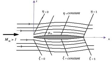
Figure 1. Right and left leaning characteristics on a thin 2D airfoil
where: η=x-nz and ζ=x+nz.
Experience has shown that the leading edge and the trailing edge of supersonic airfoils should be sharp (or only slightly rounded) and the section relatively thin. If the leading edge is not sharp (or only slightly rounded), the leading-edge shock wave will be detached and relatively strong. For the thin airfoils the thickness, camber, and angle of attack of the section are such that the local flow direction at the airfoil surface deviates only slightly from the free-stream direction.
The compressive changes in flow direction are sufficiently small that the inviscid flow is everywhere isentropic. In reality, a shock wave is formed as the supersonic flow encounters the two-dimensional double-wedge airfoil. Since the shock wave is attached to the leading edge and is planar, the downstream flow is isentropic.
If we restrict our attention to supersonic flow, the first equation of the system (17), at order 0 in ɛ, is the 2-D wave equation and has solutions of hyperbolic type. Who’s the general solution can be expressed as a sum of two arbitrary functions:
$\varphi_{0}(x, z)=F_{1}(x-n z)+F_{2}(x+n z)$ (19)
where: $n=\sqrt{M_{\infty}^{2}-1}$.
Supersonic flow is analyzed using the fact that the properties of the flow are constant along the characteristic lines x ± nz = constant. Figure 1 illustrates supersonic flow past a thin airfoil with several characteristics shown. Notice that in the linear approximation the characteristics are all parallel to one another and lie at the Mach angle μ∞ of the free stream. Information about the flow is carried in the value of the potential assigned to a given characteristic and in the spacing between characteristics for a given flow change.
All properties of the flow, velocity, pressure, temperature are constant along the characteristics. Since disturbances only propagate along downstream running characteristics we can write the velocity potential for the upper and lower surfaces. Indeed, by making the change of variables η and ζ in the first equation of the system (17), we obtain:
$\left\{\begin{array}{ll}\varphi_{0}^{+}(\eta, \xi)=F_{1}(\eta) & z \succ 0 \\ \varphi_{0}^{-}(\eta, \xi)=F_{2}(\xi) & z \prec 0\end{array}\right.$ (20)
(+) And (-) denote, respectively, the upper and lower surfaces.
Knowing that: $\frac{\partial 0}{\partial x}=\frac{\partial 0}{\partial \xi}+\frac{\partial 0}{\partial \eta}$ and $\frac{\partial()}{\partial z}=n\left(\frac{\partial 0}{\partial \xi}-\frac{\partial 0}{\partial \eta}\right)$, the slip condition (17), at order 0 in ɛ and taking into account (20), allows to obtain:
$\left\{\begin{array}{l}\varphi_{0}^{+}(\eta, \xi)=F_{1}(\eta)=-\frac{1}{n} f^{+}(\eta) \\ \varphi_{0}^{-}(\eta, \xi)=F_{2}(\xi)=\frac{1}{n} f^{-}(\xi)\end{array}\right.$ (21)
Similarly, making the change of variables η and ζ in the first equation of the system (18), we obtain:
$4 n^{2} \frac{\partial^{2} \varphi_{1}}{\partial \eta \partial \xi}=-M_{\infty}^{2}\left\{\left[(\gamma+1)+n^{2}(\gamma-1)\right]\left(\frac{\partial^{2} \varphi_{0}}{\partial \xi^{2}}+\frac{\partial^{2} \varphi_{0}}{\partial \eta^{2}}\right)\left(\frac{\partial \varphi_{0}}{\partial \xi}+\frac{\partial \varphi_{0}}{\partial \eta}\right)\right.$
$\left.+2 n^{2}\left(\frac{\partial^{2} \varphi_{0}}{\partial \xi^{2}}-\frac{\partial^{2} \varphi_{0}}{\partial \eta^{2}}\right)\left(\frac{\partial \varphi_{0}}{\partial \xi}-\frac{\partial \varphi_{0}}{\partial \eta}\right)\right\}$ (22)
The solution, at order 1 in ɛ, is obtained by integrating twice the equation (22) and taking into account the slip condition (2nd equation of the system (18)). Indeed, on the upper side, we obtain:
$\varphi_{1}^{+}(\eta, \xi)=-\frac{M_{\infty}^{4}}{8 n^{4}}(\gamma+1) \xi\left(\frac{d f^{+}}{d \eta}\right)^{2}+G^{+}(\eta)$ (23)
where:
$\frac{d G^{+}(\eta)}{d \eta}=\left(\frac{1}{n^{2}}-\frac{M_{\infty}^{4}}{8 n^{4}}(\gamma+1)\right)\left(\frac{d f^{+}}{d \eta}\right)^{2}-f^{+} \frac{d^{2} f^{+}}{d \eta^{2}}$$+\frac{M_{\infty}^{4}}{8 n^{4}}(\gamma+1) \eta \frac{d}{d \eta}\left[\left(\frac{d f^{+}}{d \eta}\right)^{2}\right]$ (24)
Similarly, on the lower side, we obtain:
$\varphi_{1}^{-}(\eta, \xi)=-\frac{M_{\infty}^{4}}{8 n^{4}}(\gamma+1) \eta\left(\frac{d f^{-}}{d \xi}\right)^{2}+G^{-}(\xi)$ (25)
where:
$\frac{d G^{-}(\xi)}{d \xi}=\left(\frac{1}{n^{2}}-\frac{M_{\infty}^{4}}{8 n^{4}}(\gamma+1)\right)\left(\frac{d f^{-}}{d \xi}\right)^{2}-f^{-} \frac{d^{2} f^{-}}{d \xi^{2}}$$+\frac{M_{\infty}^{4}}{8 n^{4}}(\gamma+1) \xi \frac{d}{d \xi}\left[\left(\frac{d f^{-}}{d \xi}\right)^{2}\right]$ (26)
Then the Mach number along the profile is defined as:The relations (21) and (23) - (26) allow to determine the velocity field at each point of the profile, and consequently to deduce the Mach number along the upper and lower surfaces. Indeed, the velocity field for the upper and lower, at order 2 in ɛ, are expressed respectively as:
$\overrightarrow{u^{+}}=\left[\begin{array}{c}1-\varepsilon \frac{1}{n} \frac{d f^{+}}{d \eta}-\varepsilon^{2} \frac{1}{n^{2}}\left(n^{2} f^{+} \frac{d^{2} f^{+}}{d \eta^{2}}+\frac{M_{\infty}^{4}}{4 n^{2}}(\gamma+1)\left[\left(\frac{d f^{+}}{d \eta}\right)^{2}-(\eta-\xi) \frac{d f^{+}}{d \eta} \frac{d^{2} f^{+}}{d \eta^{2}}\right]-\left(\frac{d f^{+}}{d \eta}\right)^{2}\right) \\ \varepsilon \frac{d f^{+}}{d \eta}+\varepsilon^{2}\left(n f^{+} \frac{d^{2} f^{+}}{d \eta^{2}}-\frac{1}{n}\left(\frac{d f^{+}}{d \eta}\right)^{2}-\frac{M_{\infty}^{4}}{4 n^{3}}(\gamma+1)(\eta-\xi) \frac{d f^{+}}{d \eta} \frac{d^{2} f^{+}}{d \eta^{2}}\right)\end{array}\right]$ (27)
And
$\overrightarrow{u^{-}}=\left[\begin{array}{cc}{1+\varepsilon \frac{1}{n} \frac{d f^{-}}{d \xi}-\varepsilon^{2} \frac{1}{n^{2}}\left(n^{2} f^{-} \frac{d^{2} f^{-}}{d \xi^{2}}+\frac{M_{\infty}^{4}}{4 n^{2}}(\gamma+1)\left[\left(\frac{d f^{-}}{d \xi}\right)^{2}+(\eta-\xi) \frac{d f^{-}}{d \xi} \frac{d^{2} f^{-}}{d \xi^{2}}\right]-\left(\frac{d f^{-}}{d \xi}\right)^{2}\right)}\\{\varepsilon \frac{d f^{-}}{d \xi}-\varepsilon^{2}\left(n f^{-} \frac{d^{2} f^{-}}{d \xi^{2}}-\frac{1}{n}\left(\frac{d f^{-}}{d \xi}\right)^{2}+\frac{M_{\infty}^{4}}{4 n^{3}}(\gamma+1)(\eta-\xi) \frac{d f^{-}}{d \xi} \frac{d^{2} f^{-}}{d \xi^{2}}\right)}\end{array}\right]$ (28)
Then the Mach number along the profile is defined as:
$M^{\pm}=M_{\infty} \frac{\|\overrightarrow{u^{\pm}}\|}{\sqrt{1+\frac{\gamma-1}{2} M_{\infty}^{2}(1-\|\overrightarrow{u^{\pm}}\|)^{2}+\mathrm{O}\left(\varepsilon^{3}\right)}}$ (29)
In relation (29), the denominator is defined at order ε3 (i.e. all terms proportional to ε3 will be neglected). We note that the model developed depends on several physical parameters as the upstream Mach number, the relative thickness and equation of the profile, and the nature of the gas.
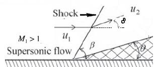
In a wide variety of physical situations, a compression shock wave occurs which is inclined at an angle to the flow. Such a wave is called an oblique shock. This type, either straight or curved, can occur in such varied examples as supersonic flow over a thin airfoil or the presence of a wedge in a supersonic stream or during a supersonic compression in a corner (see Figure 2).
Figure 2. Attached an oblique shock for a corner flow
We consider a supersonic flow passes over a slender semi-wedge of θ angle, as shown in Figure 2; the plane shock wave is formed and is inclined by an angle of β with respect to the incoming flow direction. When the upstream supersonic stream encounters a compression corner, the downstream flow is deflected by an angle δ. We note that the subscript “1” is relative to the region upstream of the shock and the subscript “2” to the region behind the shock.
Indeed, a slender semi-wedge profile, which has as dimensionless equation in, the (x, z) plane:
$z=\operatorname{tg}(\theta) x$ with $\varepsilon=\operatorname{tg}(\theta)$ (30)
The deviation angle δ is determinate, namely:
$\delta=\arccos \left(\frac{\vec{u}_{1} \cdot \vec{u}_{2}}{\left\|\vec{u}_{1}\right\|\left\|\vec{u}_{2}\right\|}\right)$ (31)
where: $\vec{u}_{1}=(1,0)$. And taking into account the relation (30) into (27) $\vec{u}_{2}$ is expressed as:
$\vec{u}_{2}=\left[\begin{array}{c}1-\frac{\operatorname{tg}(\theta)}{\sqrt{M_{1}^{2}-1}}+\operatorname{tg}^{2}(\theta)\left[\frac{1}{M_{1}^{2}-1}-\frac{(\gamma+1) M_{1}^{4}}{4\left(M_{1}^{2}-1\right)^{2}}\right] \\ \operatorname{tg}(\theta)-\frac{\operatorname{tg}^{2}(\theta)}{\sqrt{M_{1}^{2}-1}}\end{array}\right]$ (32)
Then, we can deduce:
$\delta=\arccos \left(\frac{1-\frac{\operatorname{tg}(\theta)}{\sqrt{M_{1}^{2}-1}}+\operatorname{tg}^{2}(\theta)\left[\frac{1}{M_{1}^{2}-1}-\frac{(\gamma+1) M_{1}^{4}}{4\left(M_{1}^{2}-1\right)^{2}}\right]}{\sqrt{\left(1-\frac{\operatorname{tg}(\theta)}{\sqrt{M_{1}^{2}-1}}+\operatorname{tg}^{2}(\theta)\left[\frac{1}{M_{1}^{2}-1}-\frac{(\gamma+1) M_{1}^{4}}{4\left(M_{1}^{2}-1\right)^{2}}\right]\right)^{2}+\left(\operatorname{tg}(\theta)-\frac{\operatorname{tg}^{2}(\theta)}{\sqrt{M_{1}^{2}-1}}\right)^{2}}}\right.$ (33)
In our case, for weak disturbances from presence of body, we have:
$M_{1}=\frac{1}{\sin (\beta)}=\frac{1}{\sin \left(\mu_{\infty}\right)}$ (34)
According to relations (33) and (34), δ as a unique function of θ, M1, and β. This relation is vital to an analysis of oblique shocks.
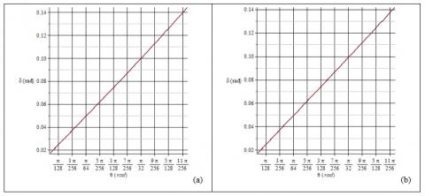
Now we will look for the relationship between the deviation angle δ and the slender semi-wedge of θ angle. For example, the value of M1 is fixed and we consider air as fluid (γ=1.4). The relationship (33) draws the δcurve as a function of θ (see figures below).
Figure 3. Relationship between the angles δ and θ. a) M1=1.4; b) M1=2
For any given M1, according to figure (3), there is a linear relation between δ delta and θ. Then:
$\delta \cong \theta$ (35)
Thus, for a supersonic flow over the wedge-shaped body, a straight, oblique shock wave is attached to the sharp nose of the wedge. Across this shock wave, the streamline direction changes discontinuously. Ahead of the shock, the streamlines are straight, parallel, and horizontal; behind the shock they remain straight and parallel but in the direction of the wedge surface.
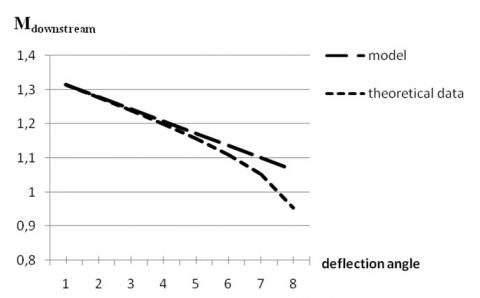
In order to validate our model, we compare the results of our model with those of the theory. Indeed, we refer to the existing theoretical data to extract different Mach number downstream. The values for downstream Mach number of oblique shock, as a function of the deflection angle and the Mach number upstream are shown in Figures 4, 5 and 6.
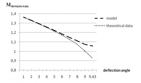
Figure 4. Weak oblique shock for Mupstream=1.35
In Figure 4, for the Mach number (Mupstream=1.35), we remark that the results of our model are in good agreement with theoretical data for a deflection angle between 0° and 5°. But beyond, a great divergence between our model and the theoretical data is observed when the downstream flow becomes subsonic.
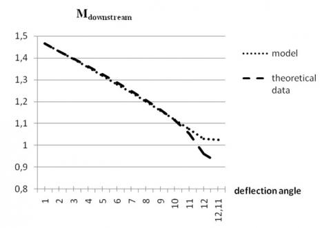
Figure 5. Weak oblique shock for Mupstream=1,4
In Figure 5, for the Mach number (Mupstream=1.4), we remark that the results of our model are in good agreement with theoretical data for a deflection angle between 1° and 7°. But beyond, a great divergence between our model and the theoretical data is observed when the downstream flow becomes subsonic.
Figure 6. Weak oblique shock for Mupstream=1.5
In Figure 6, for the Mach number (Mupstream=1.5), we observe the same phenomenon as previously. Finally, we note that in the weak shock solution, M2is supersonic, except for a small region near θmax.
Now, we consider the deflection angle θ= 1°. For different values of Mupstream, the Mdownstream of our model (at ε2order) and the Mdownstream of theoretical are presented and compared (Table 1).
Table 1. Comparison the Mdownstream of theoretical data and model results
|
Mupstream |
Mdownstream ( theoretical data) |
Mdownstream (model at $\varepsilon^{2}$ order) |
Relative error (in %) |
|
1.3 |
1.2629 |
1.262966767 |
0.007 |
|
1.35 |
1.3142 |
1.314229432 |
0.003 |
|
1.4 |
1.365 |
1.365075134 |
0.008 |
|
1.45 |
1.4156 |
1.415630095 |
0.003 |
|
1.5 |
1.466 |
1.465971748 |
0.003 |
|
1.55 |
1.5161 |
1.516150466 |
0.005 |
|
1.6 |
1.5662 |
1.566200557 |
0.001 |
|
1.65 |
1.6161 |
1.616146257 |
0.005 |
|
1.7 |
1.666 |
1.666005208 |
0.001 |
|
1.75 |
1.7158 |
1.715790578 |
0.001 |
|
1.8 |
1.7655 |
1.765512404 |
0.001 |
|
1.85 |
1.8152 |
1.815178480 |
0.002 |
|
1.9 |
1.8648 |
1.864794958 |
0.001 |
|
1.95 |
1.9144 |
1.914366748 |
0.003 |
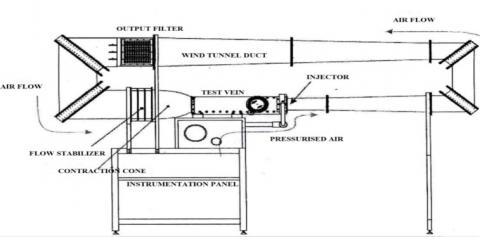
Experimentation was carried out in the AF300 supersonic wind tunnel. The test section has a rectangular shape, the top wall has the convergent-divergent profile and the bottom wall plate has 25 pressure taps, see Figure 7.
Figure 7. AF300 supersonic wind tunnel TecQuipment Company
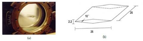
The double-wedge airfoil dimensions are 25 by 25 mm with the angle of 10°. The double-wedge airfoil is showed in Figure 8.
Figure 8. The double-wedge airfoil: (a) experimental setup; (b) dimensions (mm)
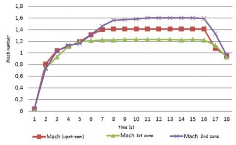
In Figure 7, circle containing double wedge airfoil represents the Schlieren window. On the other hand, with the aim to know the flow behavior in the double-wedge airfoil, an experiment was realized at 1.4 Mach number and the static pressure data were registered at this condition. The static pressure used to compute the Mach number, temperature and density in the wind tunnel test section. These results are showed in Figure 9, for upstream pressure of 0.391 bar.
Figure 9. Evolution of downstream Mach number on the dihedral airfoil
The Figure 9 presents the experimental development that includes the procedure of oblique shock. Also shows, in Figure 10b, the compression area (1st zone), and the Mach number decreases to 1.22 due at change of flow direction, while expansion area (2nd zone) the flow is accelerating to reach a 1.61 Mach number.
Figure 10. Oblique shock waves on double-wedge airfoil: (a) visualization characteristics; (b) schematic of compression and expansion zones
The Figure 10a, wave visualization characteristics in the leading edge and trailing edge on the double-wedge airfoil, at 1.4 Mach number, by means of the Schlieren method. The Mach angle in oblique shock wave in the leading edge is 46°. The shock wave is visible only on the top side of the profile.
In order to validate our model, we compare the model results with the experimental data above. Indeed, we consider a 10° angle dihedral airfoil (ϴ=5°), in which equation profile is split in two zones (Figure 10b), as:
$\left\{\begin{array}{ll}f_{1 s t \text { sone}}^{+}=x & 0 \leq x \leq 1 / 2 \\ f_{2 \text { nd zone }}^{+}=1-x & 1 / 2 \leq x \leq 1\end{array}\right.$ (36)
Then, using the relations (27) and (29), we finds according to our model that, for an upstream mach number M1= 1.4, in the compression zone M2=1.220724175 and the M3 =1.569034156 in expansion area. The estimated differences between model results and experience are, respectively, of order 0.07% in the 1st region and 4% in the 2nd region.
In this work, the two-dimensional isentropic and inviscid supersonic flow, and around a wedge has been modeled using the asymptotic analysis and characteristics method. Various parameters of our model (Mach number, deviation) were found in good agreement with the results of the theory. The results achieved demonstrate a very high accuracy: the errors $\triangle M_{\text {downstream}}=M_{\text {downstream}}^{\text {Model}}-M_{\text {downstream}}^{\text {Theory}}$ in the proposed model are estimated at about $10^{-5}$. These solutions allow us to estimate the flow parameters downstream the shock.
The exploitation of the results of the experimental study, indicates that on the first zone of the dihedral airfoil is a compression area and the second is an expansion area. The estimated differences between model results and experience are, respectively, of order 0.07% in the 1st region and 4% in the 2nd region. The acquisition of Mach number values shows a good agreement. The schlieren photographs of the shock waves were not satisfactory for quantitive comparisons with the theoretical shapes. However, definite qualitative agreement was observed.
As is evident from the comparison with the experimental data shows, our model is capable of predicting physically realistic distributions of much numbers on the airfoil.
[1] Lele, S. (1989). Direct numerical simulation of compressible free shear flows. 27th Aerospace Sciences Meeting, Aerospace Sciences Meetings, NASA, Ames Research Center, Moffett Field; Stanford University, CA, 17. https://doi.org/10.2514/6.1989-374
[2] Bartosiewicz, Y., Aidoun, Z., Desevaux, Mercadier, P. (2005). Numerical and experimental investigations on supersonic ejectors. International Journal of Heat and Fluid Flow, 26(1): 56-70. https://doi.org/10.1016/j.ijheatfluidflow.2004.07.003
[3] Khalid, M.S.U., Malik, M.A. (2009). Modeling & simulation of supersonic flow using McCormack’s technique. Proceedings of the World Congress on Engineering, II(1-3), London, U.K.
[4] Zhou, L.Q., Chen, Y.S., Chen, F.Q. (2013). Chaotic motions of a two-dimensional airfoil with cubic nonlinearity in supersonic flow. Aerospace Science and Technology, 25(1): 138-144. https://doi.org/10.1016/j.ast.2012.01.001
[5] Chen, S.X., Min, J.Z., Zang, Y.Q. (2009). Weak shock solution in supersonic flow past a wedge. American institute of Mathematical Sciences, 23(1&2): 115-132. https://doi.org/10.3934/dcds.2009.23.115
[6] Elling, V., Liu, T. (2008). Supersonic flow onto a solid wedge. Communication on Pure and Applied Mathematics, 61(10): 2008.
[7] Aliakbarov, D.T., Kukin, A.A., Trofimov, V.V. (2018). The possibility of studying supersonic flow profile close to the screen by the method of hydraulic analog modeling. Naučnyj Vestnik MGTU GA, 21(1): 60-66. https://doi.org/10.26467/2079-0619-2018-21-1-60-66
[8] Shoja-Sani, A., Roohi, E., Kahrom, M., Stefanov, S. (2014). Investigation of aerodynamic characteristics of rarefied flow around NACA 0012 airfoil using DSMC and NS solvers. European Journal of Mechanics B/Fluids, 48: 59-74. https://doi.org/10.1016/j.euromechflu.2014.04.008
[9] Zeytounian, R.K. (2002). Asymptotic modelling of fluid flow phenomena. J. Fluid Mech, 471: 409-410.
[10] Hasnaoui, M., Agouzoul, M. (2002). Linear spectral analysis of three-dimensional inhomogeneous turbulent free jet under realistic atmospheric conditions. AMSE Periodical Journal.Modelling B, 71(5): 1-22.
[11] Hasnaoui, M. (2007). Influence of Coriolis Forces on The Dynamique of A Turbulent Jet. AMSE Journal, Modelling B, 76(6): 63-76.
[12] Slimani, A., Hasnaoui, M. (2007). The gravity waves in atmospheric shear flows with Coriolis forces. AMSE Journal, Modelling B, 76(4): 20-39.
[13] Mehdari, A., Hasnaoui, M., Agouzoul, M. (2018). Dynamic behavior of flexible riser conveying oil application: Asymptotic expansion to analyze flow induced vibration (FIV). TSP (Tech Science Press), 1(1): 1-5.
[14] Caillerie, D., Cousteix, J., Mauss, J. (2016) Méthodes asymptotiques en mécanique. Edition Cépaduès, eBook ISBN : 978236493503, Ref :1503, Toulouse, France.