G. Sailaja*![]() | B. Narendra Kumar Rao
| B. Narendra Kumar Rao![]()
© 2025 The authors. This article is published by IIETA and is licensed under the CC BY 4.0 license (http://creativecommons.org/licenses/by/4.0/).
OPEN ACCESS
This study explores the application of the Extreme Gradient Boosting (XGBoost) algorithm for sentiment classification using EEG signals from the MUSE device. The model was evaluated using key performance metrics, including accuracy, precision, recall, and F1-score, achieving a notable accuracy of 99.1%. XGBoost's strengths in processing large datasets, reducing over fitting through regularization, and effectively handling EEG data are highlighted. The results underscore the effectiveness of ensemble learning methods in improving human-computer interaction and advancing emotional processing. There is significant potential for integrating real-time EEG-based sentiment analysis into interactive systems and wearable technologies, with promising applications in gaming, healthcare, and mental health monitoring. This research contributes to the development of intelligent, adaptive AI-driven systems and lays a solid foundation for future EEG-based emotion recognition technologies.
emotion recognition, EEG-based classification, physiological signals, XGBoost, emotion recognition, affective computing, mental health monitoring
Emotions are an essential component of human existence, significantly influencing daily experiences and decision-making. Models for emotion recognition aim to understand and respond to human emotions, with applications across domains such as driver monitoring, healthcare, entertainment, and software user experience enhancement [1] These models commonly rely on two main approaches: behavioral and physiological. Behavioral methods recognize emotions through facial expressions and gestures, while physiological approaches use biological signals such as electrodermal activity (EDA), galvanic skin response (GSR), electrocardiography (ECG), and electroencephalography (EEG). Unlike behavioral indicators, physiological signals are continuously accessible and cannot be consciously controlled. Combining both approaches leads to a more comprehensive understanding of an individual’s emotional state [2].
Many studies focus on emotion recognition by examining subjects’ responses to controlled stimuli in laboratory settings. However, accurately identifying emotions in real-world environments remains challenging. EEG signals provide valuable insights into emotions that may not be verbally expressed. EEG measures electrical activity via electrodes placed on the scalp, capturing signals primarily from pyramidal neurons in the cortex. These signals reflect the summed potentials of excitatory and inhibitory postsynaptic currents of neurons near each electrode. Because EEG reflects brain activity in response to stimuli or events, it is a powerful tool for emotion classification [3].
Various machine learning methods have been applied to EEG-based emotion recognition, but the use of XGBoost in this domain has been limited. XGBoost offers advantages such as modeling non-linear EEG patterns, robustness to noise, and built-in regularization to reduce over fitting, making it promising for real-time emotion detection from physiological signals. EEG-based emotion recognition also holds potential for enhancing the diagnosis and treatment of neurological and psychological disorders such as stroke, stress, epilepsy, mood disorders, and anxiety. It is especially beneficial for understanding emotional states in neuro diverse populations. This study adopts an interdisciplinary approach, integrating computational, psychological, and neurophysiological models to advance emotion recognition methods [4].
An examination of current research on EEG-based emotion recognition features progress in this field, covering aspects like signal processing, feature extraction, classification techniques, and practical applications. Our extensive literature review explores advancements in EEG-based emotion recognition, highlighting emerging trends, challenges, and significant achievements in this multidisciplinary domain [5]. Researchers continually strive to improve the accuracy, reliability, and real-world relevance of EEG-based emotion recognition systems.
Early studies focused on whether emotional states could be identified from brainwave patterns. Numerous studies have examined the relationship between emotional experiences and brain activity, particularly in the frontal regions. Frontal EEG asymmetry has been investigated as a potential biomarker for vulnerability to depression. Although frontal asymmetry may help identify individuals at risk for depression, further large-scale longitudinal studies are necessary to validate these findings [6]. Research in this area also supports the advancement of personalized, neuroscience-based treatment strategies. By analyzing neural activity changes, researchers can evaluate intervention effectiveness, including psychotherapy, in modulating brain networks.
Studies on frontal alpha asymmetry have further explored neuro feedback training as a tool for reducing anxiety and negative emotions. For example, one study investigated the effects of neuro feedback training on depression, anxiety, and affect by analyzing specific changes in alpha wave power across different frontal regions [7] as shown in below Figure 1.
Figure 1. Frontal EEG asymmetry
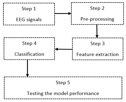
These pioneering studies pave the way for future EEG-based research on the neural mechanisms underlying emotions. Numerous investigations have focused on signal processing techniques to enhance EEG data accuracy in emotion recognition, as illustrated in Figure 2 researchers have developed various methods to improve EEG signal quality by eliminating artifacts such as eye blinks, muscle movements, and environmental noise, thereby increasing the accuracy and reliability of emotion recognition systems [8].
Figure 2. Human emotions identification and recognition using EEG signal processing
3.1 XGBoost algorithm
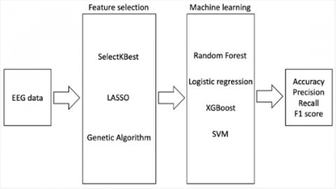
This examination utilizes the eXtreme Gradient Boosting (XGBoost) algorithm for emotion classification. XGBoost is widely recognized for its effectiveness and efficiency in processing large datasets and handling complex models. Built on the principles of gradient boosting, it combines linear model solvers with tree-based learning techniques, making it a powerful choice for this task [9]. This section explores the application of XGBoost in EEG-based emotion classification, as shown in Figure 3. Known for its adaptability and strong performance across various machine learning applications, XGBoost has proven to be highly effective in sentiment analysis using EEG signals.
Figure 3. EEG brainwave dataset training
3.1.1 Application of XGBoost algorithm for EEG-based sentiment classification
XGBoost employs a boosting ensemble learning approach, where multiple weak models are constructed sequentially to correct errors from previous iterations [10]. This iterative improvement enables XGBoost to achieve high predictive accuracy, making it a dependable option for sentiment classification tasks.
A key advantage of XGBoost is its efficiency in processing complex datasets. By integrating regularization techniques, it reduces the bet of over fitting and manages the model's hypothesis to new data [11]. Furthermore, XGBoost is equipped to manage missing values effectively, ensuring robustness even when dealing with incomplete data [12].
Furthermore, XGBoost is highly scalable and supports parallel processing, making it well-suited for large datasets. Its adaptability and strong performance have made it a widely used algorithm across various machine learning applications. In EEG-based sentiment classification, XGBoost is particularly effective at detecting subtle patterns within EEG signals. Since EEG data often exhibits non-linear relationships, the gradient boosting technique employed by XGBoost captures intricate interactions and dependencies, leading to more accurate emotion classification.
XGBoost is commonly utilized in supervised learning tasks, where the training data includes input features (x) paired with corresponding target labels (y). One of the model's goals is to learn a function that accurately predicts based on x [13]. The mathematical formulation of XGBoost can be represented as follows:
$\mathrm{y}_{\mathrm{i}}=\sum_{k=0} f k\left(x_i\right), \mathrm{f}_k € \mathrm{U}$
where, F denotes the space of regression trees, and fk(xi) is the prediction of the k-th tree for the input xi.”
This equation represents the aggregation process in XGBoost, where the total number of trees in the mode is indicated by k. Each tree’s prediction, represented as fk belongs to the function space U. The model iterates through all k trees in the ensemble, summing their individual predictions for a given input data point xi. This results in the final predicted value yi which is obtained as the cumulative outcome of all tree-based predictions [14].
3.1.2 Model evaluation
We will start by creating a classification report that includes important performance indicators for every class, such as F1-score, precision, and recall. This report considers the examination of the model's show across various classes and helps identify potential biases or imbalances in its predictions.
We will then create a confusion matrix to examine the model's performance graphically. The confusion matrix provides information about the distribution of accurate and inaccurate predictions across different classes by contrasting predicted and actual labels [15]. This makes it easier to spot misclassification trends and evaluate the model's overall accuracy.
By leveraging both classification report and confusion matrix, we aim to obtain a thorough evaluation of our XGBoost model’s strengths and limitations. These insights will guide decisions regarding its optimization and deployment in real-world applications [16].
3.2 Metrics for performance
The viability of EEG-based feeling recognition models is assessed using various performance metrics. Commonly used metrics such as recall, accuracy, precision and F1-score, indicate the model's ability to classify different emotional states accurately. In multiclass EEG-based emotion classification scenario each class represents a distinct emotional category [17].
True negatives (TN) occur when the model correctly identifies that a model doesn't have a spot with a specific class, while true positives (TP) refer to instances where the model accurately detects a given class [18]. False negatives (FN) indicate cases where the model neglects to perceive occasions of a specific class, whereas false positives (FP) occur when the model erroneously orders an example as having a place with a class [19].
The following definitions apply to performance metrics like accuracy, precision, recall, F1-score, and the confusion matrix:
1. Consistency: Consistency evaluates the model's general capacity to precisely anticipate class names. The level of accurately ordered examples relative to all instances is the definition of multiclass classification. The following is the formula for Consistency:
$Accuracy =\frac{T P+F p}{{TN}+\mathrm{TP}+{FP}+{FN}}$
2. Precision (P): By computing the extent of accurately grouped positive examples to all occurrences anticipated as certain, accuracy surveys how precise the model's positive forecasts are. This formula is used to calculate it:
$Precision=\frac{T P}{{TP}+{FP}}$
3. Recall (R): The model's capacity to perceive each case of a particular class is estimated by review. It shows the level of genuine positive cases that the model precisely distinguished
$Recall =\frac{T P}{T P+F N}$
4. F1-score: The model's show is surveyed extensively by changing the precision of positive figures and its capacity to unequivocally recognize authentic positive models across all classes. The F1-score is the consonant mean of precision and survey
$F 1=2 \mathrm{X} \frac{P X R}{{P}+{R}}$
5. Confusion matrix (CM): A confusion matrix is a tabular representation that evaluates the performance of a classification model by comparing its predicted labels with the actual labels.
The XGBoost model demonstrated outstanding performance, achieving an accuracy of 99.1% when trained with selected features, highlighting its effectiveness in sentiment classification across the dataset [20]. The classification report provides a comprehensive evaluation of the model’s performance. It presents key metrics such as precision, recall, and F1-score for each class (negative, neutral, and positive), demonstrating the model’s ability to accurately classify instances [21]. Furthermore, both the macro and weighted average F1-scores reached 0.99, as shown in Table 1, further confirming the model’s robust overall performance across all sentiment categories [22].
Table 1. The classification report for XGBoost model
|
Classification Report for XGBoost Model |
||||
|
Features |
Precision |
Recall |
F1-Score |
Support |
|
id_0 |
0.98 |
0.98 |
0.98 |
201 |
|
id_1 |
1.00 |
0.98 |
1.00 |
231 |
|
id_2 |
0.97 |
0.98 |
0.96 |
208 |
|
Accuracy |
0.99 |
640 |
||
|
Macro average |
0.99 |
0.99 |
0.99 |
640 |
|
Average weight |
0.99 |
0.99 |
0.99 |
640 |
Furthermore, the Confusion matrix provides valuable insights into the model's characterization execution [23], as shown in Table 2. The high qualities along the inclining demonstrate proper expectations, whereas the off-corner to corner components are misclassified cases [24]. The distribution of values within the grid demonstrates the model's strong ability to precisely order occurrences across all feeling classifications.
Table 2. The confusion matrix for XGBoost
|
|
Predicted Labels |
|||||
|
|
N1 |
N2 |
N3 |
R |
W |
|
|
True Labels |
N1 |
0.46 |
0.007 |
0.00 |
0.32 |
0.15 |
|
N2 |
0.01 |
0.76 |
0.08 |
0.15 |
0.00 |
|
|
N3 |
0.00 |
0.08 |
0.91 |
0.00 |
0.00 |
|
|
R |
0.06 |
0.17 |
0.00 |
0.74 |
0.02 |
|
|
W |
0.13 |
0.00 |
0.00 |
0.05 |
0.82 |
|
where, N1: Negative sentiment, N2: Neutral sentiment N3: Positive sentiment, R: Resting or baseline state W: Wakeful or alert state
In conclusion, XGBoost's adaptability, scalability, and capability to capture non-linear relationships make it a highly effective tool for EEG-based sentiment classification, enabling accurate inference of emotional states from EEG data. To assess the performance of the integrated XGBoost model, the classification report and confusion matrix are employed as key evaluation metrics, providing a comprehensive understanding of model accuracy and misclassification trends [25].
Overall, the results highlight the model’s precision and practicality in sentiment classification tasks, demonstrating its potential for real-world applications in emotion recognition and related domains such as healthcare, education, and user experience systems. This study uses only publicly available secondary data and does not involve human participants. Hence, ethical approval and informed consent are not applicable, consistent with prior EEG studies utilizing open-access datasets.
The code implements a series of functions to assess machine learning models on a specified dataset. The generate_generic_results function performs leave-one-subject-out evaluations, in this case, models are trained using information from every subject except the one being assessed, tested on the excluded subject, and the results are stored. The generate_combined_general_results function assesses models across the entire dataset using cross-validation and saves the outcomes. Both functions rely on utilities from an utils module for tasks such as data preprocessing, model management, and performance evaluation. The type of models used is defined by the model type, and the results are organized in directories for further analysis. A key limitation of the study is the exclusion of several smaller states and union territories due to data unavailability. This may introduce a small sample bias and limit the representativeness of the findings across all Indian regions. Future studies could aim to include a broader set of regions or utilize alternative data sources to enhance generalizability.
4.1 PLOTS-swell
The function for calibrating and evaluating machine learning models on EEG data. The calibrate_model function combines generic and calibration data to retrain models with fresh parameters. The get_data function loads dataset files, while generate_calibration_results tests model performance across various sample sizes and saves the results. The calibration process ensures models are optimized [26] for better accuracy in predictions.
4.2 Exploratory Data Analysis (EDA)
This portion dives into the Exploratory Data Analysis (EDA) phase, offering insights into the features of the EEG dataset [1]. Descriptive statistics, visualizations, and key observations are provided to deliver a thorough analysis of the data's distribution, patterns, and potential challenges. The EDA of the EEG-based emotion classification dataset, comprising 2132 observations and 2549 features, revealed a well-distributed label distribution with approximately 33.6% for neutral sentiments and 33.2% each for positive and negative sentiments. The absence of missing values and the wide span of numerical representations contribute to the dataset’s complexity. The relationship between calibration samples per subject and model performance—including classification accuracy, precision, mean absolute error, and root mean square error—has been investigated in prior studies emphasizing the importance of personalized EEG data interpretation. (see Figures 4 and 5).
Figure 4. EDA-model calibration
Figure 5. HRA-model calibration
4.3 PLOTS-wesad
The code evaluates machine learning models on EEG data with a focus on individual subject performance. It utilizes cross-validation to compute various evaluation metrics for each subject, as recommended in prior studies involving subject-dependent EEG emotion recognition [27]. The get_cross_val_results function assesses model accuracy, while the generate_person_specific_results function trains models on data from each subject and saves the outcomes, a method consistent with personalized EEG classification strategies [28]. It processes multiple datasets, signal types, and model types to provide detailed performance evaluations for each subject, which is crucial for enhancing model generalization and robustness in EEG-based emotion recognition systems [29].
Figure 6 demonstrates high classification accuracy and low regression errors with minimal calibration data, indicating strong model adaptability, while Figure 7 summarizes subject-specific model evaluations using cross-validation and performance metrics across various signals and models [30].
Figure 6. EDA-model calibration
Figure 7. HRA-model calibration
EEG-based emotion recognition has evolved into a multidisciplinary domain that integrates neuroscience, psychology, and machine learning to effectively interpret and classify emotional states. Progress in signal processing and classification methods has greatly enhanced the reliability of these systems, with frontal EEG asymmetry emerging as a key indicator of emotional responses. This progress has opened up new opportunities in areas such as mental health monitoring, affective computing, and human-computer interaction.
In this context, the present study demonstrates the strong performance of the XGBoost algorithm for emotion classification using EEG signals collected from the MUSE wearable device, achieving a high accuracy of 99.1%. The use of ensemble learning enables the model to capture complex emotional patterns while minimizing overfitting, underscoring the potential of artificial intelligence to analyze emotional states and support practical applications in healthcare, user experience optimization, and intelligent adaptive systems.
Although the XGBoost model achieves high accuracy on the MUSE EEG dataset, future studies should aim to assess its applicability to external datasets and real-world environments. This includes addressing challenges such as variability between individuals, signal interference, and implementation in wearable or interactive platforms. Validating the model under these diverse conditions will be crucial to ensure its reliability and flexibility in practical sentiment analysis applications.
Future research should focus on improving model generalization by incorporating diverse datasets and real-world scenarios. Integrating real-time EEG analysis into wearable devices can enhance practical applications, enabling adaptive and personalized user experiences. Further advancements in AI-driven emotion recognition will pave the way for innovative solutions in healthcare, gaming, education, and interactive systems, fostering a more intuitive and emotionally responsive technology landscape.
Appendix-1
Sample Dataset
|
ID |
TP9 |
AF7 |
AF8 |
TP10 |
LABEL |
|
0 |
24.83 |
-6.91 |
39.04 |
93.34 |
Focused |
|
1 |
-13.22 |
62.04 |
7.17 |
-8.64 |
Relaxed |
|
2 |
29.62 |
-51.87 |
-6.98 |
-37.47 |
Stressed |
|
3 |
-71.27 |
-65.28 |
-16.23 |
54.67 |
Focused |
|
4 |
61.17 |
4.63 |
20.23 |
19.29 |
Relaxed |
|
5 |
-18.43 |
-37.28 |
9.92 |
67.65 |
Stressed |
|
6 |
-21.2 |
-71.28 |
-16.75 |
42.88 |
Relaxed |
|
7 |
-6.93 |
35.87 |
55.78 |
-11.7 |
Relaxed |
|
8 |
8.71 |
-25.9 |
22.93 |
0.25 |
Focused |
|
9 |
39.49 |
-13.92 |
62.61 |
-34.46 |
Relaxed |
|
10 |
-70.08 |
15.86 |
-34.32 |
52.79 |
Stressed |
|
11 |
3.47 |
-35.62 |
24.89 |
10.11 |
Relaxed |
|
12 |
-19.45 |
66.24 |
-16.47 |
23.97 |
Stressed |
|
13 |
11.71 |
3.39 |
17.29 |
-62.73 |
Focused |
|
14 |
-24.49 |
-5.25 |
2.29 |
-7.64 |
Relaxed |
|
15 |
8.53 |
-21.9 |
-31 |
-57.71 |
Focused |
|
16 |
-56.08 |
33.17 |
-19.15 |
20.44 |
Relaxed |
|
17 |
9.1 |
-30.15 |
-5.8 |
13.96 |
Focused |
|
18 |
31.5 |
19.36 |
29.07 |
12.56 |
Focused |
|
19 |
-29.45 |
15.28 |
-45.9 |
3.32 |
Relaxed |
|
20 |
-15.08 |
27.19 |
43.74 |
46.16 |
Stressed |
|
21 |
7.91 |
-20.6 |
23.12 |
4.42 |
Focused |
|
22 |
-58.7 |
-41.04 |
17.32 |
32.61 |
Stressed |
|
23 |
17.58 |
27.01 |
34.25 |
42.55 |
Relaxed |
|
24 |
34.46 |
10.1 |
21.01 |
-3.18 |
Relaxed |
|
25 |
-16.37 |
-40.04 |
-47.23 |
29.61 |
Focused |
|
26 |
-27.46 |
-19.67 |
-60.48 |
28.37 |
Focused |
|
27 |
-10.89 |
-10.65 |
-22.88 |
6.79 |
Stressed |
|
28 |
0.95 |
19.84 |
47.59 |
5.01 |
Relaxed |
|
29 |
15.78 |
30.05 |
-0.31 |
-15.71 |
Focused |
|
30 |
-7.46 |
2.71 |
-36.86 |
3.76 |
Focused |
|
31 |
47.57 |
0.5 |
-0.34 |
-3.97 |
Focused |
|
32 |
-43.47 |
1.84 |
2.28 |
-30.07 |
Relaxed |
|
33 |
30.44 |
28.7 |
7.99 |
3.74 |
Stressed |
|
34 |
8.95 |
-14.67 |
16.86 |
4.87 |
Focused |
|
35 |
4.13 |
32.59 |
17.63 |
21.03 |
Relaxed |
|
36 |
-1.31 |
-37.32 |
8.9 |
-0.46 |
Stressed |
|
37 |
34.9 |
-2.82 |
-1.53 |
-12.01 |
Focused |
|
38 |
26.12 |
19.32 |
-3.03 |
-7.47 |
Relaxed |
|
39 |
-19.06 |
2.55 |
-25.87 |
-6.82 |
Relaxed |
|
40 |
-7.11 |
24.71 |
-30.18 |
10.45 |
Focused |
|
41 |
7.92 |
9.67 |
11.91 |
-10.37 |
Stressed |
|
42 |
13.23 |
17.48 |
4.53 |
-4.46 |
Relaxed |
|
43 |
-36.24 |
2.32 |
2.23 |
3.68 |
Relaxed |
|
44 |
-15.32 |
-11.02 |
3.27 |
-2.41 |
Focused |
|
45 |
-19.53 |
12.18 |
-19.8 |
11.42 |
Stressed |
|
46 |
-32.77 |
-8.73 |
14.5 |
6.27 |
Relaxed |
|
47 |
21.37 |
24.91 |
18.17 |
10.18 |
Focused |
|
48 |
23.49 |
18.27 |
-5.08 |
3.2 |
Stressed |
|
49 |
30.65 |
-5.62 |
16.58 |
-5.34 |
Relaxed |
|
50 |
-15.91 |
12.62 |
-2.97 |
7.1 |
Relaxed |
|
51 |
18.34 |
-22.93 |
-23.01 |
-5.08 |
Focused |
|
52 |
-3.82 |
-2.09 |
5.81 |
2.18 |
Stressed |
|
53 |
15.1 |
13.88 |
8.06 |
8.01 |
Relaxed |
|
54 |
2.74 |
-8.79 |
-17.51 |
4.65 |
Focused |
|
55 |
19.43 |
16.32 |
15.03 |
-2.84 |
Relaxed |
|
56 |
-10.39 |
2.49 |
2.15 |
5.49 |
Focused |
|
57 |
13.28 |
-15.29 |
-1.13 |
3.87 |
Focused |
|
58 |
-22.03 |
12.19 |
-17.44 |
2.1 |
Stressed |
|
59 |
14.62 |
8.9 |
-12.17 |
6.12 |
Relaxed |
|
60 |
-2.36 |
-0.84 |
7.65 |
2.77 |
Relaxed |
|
61 |
1.28 |
5.26 |
-1.09 |
-0.79 |
Relaxed |
|
62 |
-6.77 |
-5.34 |
13.07 |
2.44 |
Stressed |
|
63 |
4.91 |
9.04 |
7.51 |
-0.22 |
Relaxed |
|
64 |
10.41 |
10.84 |
-4.99 |
2.49 |
Focused |
|
65 |
-8.73 |
3.29 |
6.29 |
-0.49 |
Relaxed |
|
66 |
7.39 |
-1.17 |
-0.65 |
-0.78 |
Focused |
|
67 |
2.12 |
4.63 |
1.23 |
3.59 |
Stressed |
|
68 |
-6.31 |
2.83 |
-4.37 |
0.62 |
Relaxed |
|
69 |
3.82 |
-0.22 |
4.73 |
-1.07 |
Relaxed |
|
70 |
0.46 |
3.95 |
3.77 |
-0.55 |
Stressed |
|
71 |
-0.32 |
-2.91 |
1.18 |
2.26 |
Focused |
|
72 |
6.7 |
-1.83 |
-0.41 |
-1.26 |
Focused |
|
73 |
-3.74 |
3.68 |
2.19 |
0.77 |
Relaxed |
|
74 |
4.14 |
-2.56 |
-0.86 |
-0.53 |
Focused |
|
75 |
-2.39 |
2.48 |
0.86 |
1.79 |
Relaxed |
|
76 |
1.41 |
-2 |
-0.99 |
-0.28 |
Relaxed |
|
77 |
-0.53 |
3.41 |
2.11 |
0.19 |
Focused |
|
78 |
5.46 |
-3.79 |
1.63 |
-0.32 |
Focused |
|
79 |
-0.81 |
0.75 |
0.62 |
-1.04 |
Relaxed |
|
80 |
1.39 |
1.28 |
-1.27 |
1.27 |
Relaxed |
|
81 |
-1.32 |
-2.91 |
3.68 |
2.79 |
Focused |
|
82 |
2.57 |
3.17 |
2.69 |
-0.67 |
Relaxed |
|
83 |
-2.84 |
0.19 |
1.37 |
1.46 |
Stressed |
|
84 |
3.96 |
1.24 |
-2.67 |
-0.79 |
Relaxed |
|
85 |
-2.45 |
2.51 |
3.28 |
1.79 |
Relaxed |
|
86 |
1.67 |
-1.9 |
0.73 |
-1.28 |
Focused |
|
87 |
-0.53 |
3.05 |
2.87 |
0.24 |
Relaxed |
|
88 |
4.18 |
-1.27 |
-0.84 |
-0.46 |
Relaxed |
|
89 |
-1.22 |
3.12 |
1.9 |
1.29 |
Focused |
|
90 |
0.57 |
-1.76 |
-0.61 |
-0.37 |
Focused |
|
91 |
3.29 |
2.24 |
-1.43 |
1.1 |
Relaxed |
|
92 |
-0.44 |
-0.74 |
3.42 |
1.64 |
Relaxed |
|
93 |
2.94 |
-2.13 |
1.31 |
-0.88 |
Focused |
|
94 |
-2.51 |
2.73 |
2.51 |
1.37 |
Relaxed |
|
95 |
3.62 |
0.91 |
-1.9 |
-0.92 |
Relaxed |
|
96 |
-1.78 |
2.91 |
3.19 |
1.7 |
Focused |
|
97 |
4.49 |
-2.29 |
0.41 |
-0.84 |
Focused |
|
98 |
-0.24 |
2.41 |
2.09 |
0.72 |
Relaxed |
|
99 |
1.8 |
0.94 |
-1.76 |
1.07 |
Relaxed |
Algorithm: XG Boost(eXtreme Gradient Boosting)
Step 1: Initialize a simple model
Start with an initial prediction for all samples.
For classification, it could be uniform probabilities.
For example, 3 classes (Relaxed, Focused, Stressed), initial prediction:
y^i(0)=1/3 for each class
Step 2: Calculate the Loss Function
We want to minimize a loss.
For classification, typically Log Loss (also called cross-entropy):
Loss $=-\sum_{i=1}^n \sum_{K=1}^n$ yik $\log \left(\mathrm{y}^{\wedge}{ }_{\mathrm{ik}}\right)$
where,
n = number of samples
K = number of classes
yik= 1 if sample i belongs to class k, else 0
y^ik = predicted probability of sample i belonging to class k
Step 3: Calculate Gradient and Hessian
To improve the model, we calculate:
If ℓ is the loss function:
Step 4: Build a Small Decision Tree
Using gi and hi XGBoost builds a small tree that predicts where the errors are.
At each split (e.g., splitting on TP9 > 320), XGBoost chooses the best split that gives the highest gain.
Gain formula:
Gain=1/2[((GL)2/(HL+λ))+ ((GR)2/(HR+λ))−((GL+GR)2/ (HL+HR+λ))]−γ
where,
GL, HL=sum of gradients and hessians for left node
GR, HR=sum of gradients and hessians for right node
λ=Regularization term
γ=cost for adding a leaf node( to control complexity)
Pick the split that maximizes the Gain.
Step 5: Update the Predictions
Once the new tree is built, the model updates its predictions:
y^i(t)=y^i(t−1)+η⋅ft(xi)
where,
η=learning rate (a small number, like 0.1)
ft(xi) = prediction from the new tree
Step 6: Repeat
Repeat for N trees (like 100–1000) or until the loss stops improving
Appendix-2
Working Model: Step-by-Step
Step1:
Using XGBoost with one tree (n_estimators=1), class probabilities were initially assigned as:
Focused: 0.3414
Relaxed: 0.3293
Stressed: 0.3293
Step2:
For any sample iii, the true class has yik=1, so:
log(y^ik) =log(1/3)≈−1.0986
$\operatorname{LogLosS}=-1 / \mathrm{n} \sum_{i=1}^n \log \left(\frac{1}{3}\right)=-\log (1 / 3)=\log (3)=1.0986$
Step3:
Given initial predictions:
y^i,Focused=0.3414
y^i,Relaxed=0.3293
y^i,Stressed=0.3293y^
Case Study i:
Sample 0: Label = Relaxed
y=[0,1,0]
Gradients gik= y^ik- yik
Focused: 0.3414−0=0.3414
Relaxed: 0.3293−1=−0.6707
Stressed: 0.3293−0=0.3293
Hessians hik= y^ik (1- y^ik)
Focused: 0.3414⋅(1−0.3414)=0.2247
Relaxed: 0.3293⋅(1−0.3293)=0.2207
Stressed: 0.3293⋅(1−0.3293)= 0.2207
Case Study ii:
Sample 1: Label = Stressed
y=[0,0,1]
Gradients:
Focused: 0.3414−0=0.34140.3414−0=0.3414
Relaxed: 0.3293−0=0.32930.3293−0=0.3293
Stressed: 0.3293−1=−0.67070.3293−1=−0.6707
Hessians:
Same as above (only depend on predicted prob):
Focused: 0.2247
Relaxed: 0.2207
Stressed: 0.2207
Case Study iii:
Sample 2: Label = Focused
y=[1,0,0]y=[1,0,0]
Gradients:
Focused: 0.3414−1=−0.65860.3414−1=−0.6586
Relaxed: 0.3293−0=0.32930.3293−0=0.3293
Stressed: 0.3293−0=0.32930.3293−0=0.3293
Hessians:
Focused: 0.2247
Relaxed: 0.2207
Stressed: 0.2207
Summary about case studies i,ii,iii
|
Sample |
Class |
Gradient |
Hessian |
|
0 |
Focused |
0.3414 |
0.2247 |
|
0 |
Relaxed |
-0.6707 |
0.2207 |
|
0 |
Stressed |
0.3293 |
0.2207 |
|
1 |
Focused |
0.3414 |
0.2247 |
|
1 |
Relaxed |
0.3293 |
0.2207 |
|
1 |
Stressed |
-0.6707 |
0.2207 |
|
2 |
Focused |
-0.6586 |
0.2247 |
|
2 |
Relaxed |
0.3293 |
0.2207 |
|
2 |
Stressed |
0.3293 |
0.2207 |
Step4:
Split at Feature0 ≤ 0.55
Left Node (samples 0,1):
GL=0.3414+0.3414=0.6828
HL=0.2247+0.2247=0.4494
Right Node (samples 2,3):
GR=−0.6586+(−0.6586)=−1.3172
HR=0.2247+0.2247=0.4494
Parent Node:
G=−0.6344, H=0.8988
Assume λ=1, γ=0
Compute Gain:
Gain=1/2[((GL)2/(HL+λ))+ ((GR)2/(HR+λ))−((GL+GR)2/ (HL+HR+λ))]−γ
=1/2[((0.6828)2/(0.4494+1))+ ((-1.3172)2/(0.4494+1)−((-0.6344)2/ (0.8988+1))]−0
= 0.6533
Leaf Value Calculation:
wL=− (0.6828/0.4494+1 ≈−0.471
wR=− (−1.31720/.4494+1≈+0.910
Step5:
Assume: Learning rate η=0.1
y^i(t)=y^i(t−1)+η⋅ft(xi)
Current prediction for class Focused = −1.0986
Tree output (leaf value) for sample 0, class Focused=0.4
y^Stressed(1)=−1.0986+0.1×0.4=−1.0986+0.04=−1.0586
Step6: Repeat for N trees (like 100–1000) or until the loss stops improving
Appendix-3
Summary of Code Implementation Details
|
Category |
Details Mentioned / Inferred |
|
Hyper parameters |
- Not explicitly stated in the manuscript. |
|
Feature Engineering |
- TF-IDF |
|
NoiseRemoval Techniques |
- Lowercasing |
|
Machine Learning Models |
- Naive Bayes |
|
Pre-processing Steps |
- Tokenization |
[1] Bos, D.O. (2006). EEG-based emotion recognition. The Influence of Visual and Auditory Stimuli, 56(3): 1-17.
[2] Cousin, E., Peyrin, C., Pichat, C., Lamalle, L., Le Bas, J. F., Baciu, M. (2007). Functional MRI approach for assessing hemispheric predominance of regions activated by a phonological and a semantic task. European Journal of Radiology, 63(2): 274-285. https://doi.org/10.1016/j.ejrad.2007.01.030
[3] Ayşe, E.K.İ.M., Aydemi̇r, Ö., Demi̇r, M. (2020). Classification of cognitive fatigue with EEG signals. In 2020 Medical Technologies Congress (TIPTEKNO), Antalya, Turkey, pp. 1-4. https://doi.org/10.1109/TIPTEKNO50054.2020.9299239
[4] Buckingham, C.D., Ahmed, A., Adams, A. (2013). Designing multiple user perspectives and functionality for clinical decision support systems. In 2013 Federated Conference on Computer Science and Information Systems, Krakow, Poland, pp. 211-218.
[5] Dhara, T., Singh, P.K. (2023). Emotion recognition from EEG data using hybrid deep learning approach. In Frontiers of ICT in Healthcare: Proceedings of EAIT 2022, Springer, Singapore, pp. 179-189. https://doi.org/10.1007/978-981-19-5191-6_15
[6] Batouli, S.A.H., Hasani, N., Gheisari, S., Behzad, E., Oghabian, M.A. (2016). Evaluation of the factors influencing brain language laterality in presurgical planning. Physica Medica, 32(10): 1201-1209. https://doi.org/10.1016/j.ejmp.2016.06.008
[7] Gallagher, A., Tanaka, N., Suzuki, N., Liu, H., Thiele, E.A., Stufflebeam, S.M. (2013). Diffuse cerebral language representation in tuberous sclerosis complex. Epilepsy Research, 104(1-2): 125-133. https://doi.org/10.1016/j.eplepsyres.2012.09.011
[8] Iyer, A., Das, S.S., Teotia, R., Maheshwari, S., Sharma, R.R. (2023). CNN and LSTM based ensemble learning for human emotion recognition using EEG recordings. Multimedia Tools and Applications, 82(4): 4883-4896. https://doi.org/10.1007/s11042-022-12310-7
[9] Jansma, J.M., Ramsey, N., Rutten, G.J. (2015). A comparison of brain activity associated with language production in brain tumor patients with left and right sided language laterality. Journal of Neurosurgical Sciences, 59(4): 327-335.
[10] Kumar, M., Molinas, M. (2022). Human emotion recognition from EEG signals: model evaluation in DEAP and SEED datasets. In Proceedings of the First Workshop on Artificial Intelligence for Human-Machine Interaction (AIxHMI 2022) co-located with the 21th International Conference of the Italian Association for Artificial Intelligence (AI* IA 2022), CEUR Workshop Proceedings, CEU.
[11] El-Nasr, M.S., Yen, J., Ioerger, T.R. (2000). Flame—Fuzzy logic adaptive model of emotions. Autonomous Agents and Multi-Agent Systems, 3: 219-257. https://doi.org/10.1023/A:1010030809960
[12] Li, H., Qing, C., Xu, X., Zhang, T. (2017). A novel DE-PCCM feature for EEG-based emotion recognition. In 2017 International Conference on Security, Pattern Analysis, and Cybernetics (SPAC), Shenzhen, China, pp. 389-393. https://doi.org/10.1109/SPAC.2017.8304310
[13] Kulkarni, S., Patil, P.R. (2021). Analysis of DEAP dataset for emotion recognition. In International Conference on Intelligent and Smart Computing in Data Analytics: ISCDA 2020, Springer, Singapore, pp. 67-76. https://doi.org/10.1007/978-981-33-6176-8_8
[14] Koelstra, S., Muhl, C., Soleymani, M., Lee, J.S., Yazdani, A., Ebrahimi, T., Patras, I. (2011). DEAP: A database for emotion analysis; using physiological signals. IEEE Transactions on Affective Computing, 3(1): 18-31. https://doi.org/10.1109/T-AFFC.2011.15
[15] Noachtar, S., Borggraefe, I. (2009). Epilepsy surgery: A critical review. Epilepsy & Behavior, 15(1): 66-72. https://doi.org/10.1016/j.yebeh.2009.02.028
[16] Wang, J., Wang, M. (2021). Review of the emotional feature extraction and classification using EEG signals. Cognitive Robotics, 1: 29-40. https://doi.org/10.1016/j.cogr.2021.04.001
[17] Wada, J.A., Clarke, R., Hamm, A. (1975). Cerebral hemispheric asymmetry in humans: Cortical speech zones in 100 adult and 100 infant brains. Archives of Neurology, 32(4): 239-246.
[18] Li, M., Lu, B.L. (2009). Emotion classification based on gamma-band EEG. In 2009 Annual International Conference of the IEEE Engineering in Medicine and Biology Society, Minneapolis, MN, USA, pp. 1223-1226. https://doi.org/10.1109/IEMBS.2009.5334139
[19] Mennella, R., Patron, E., Palomba, D. (2017). Frontal alpha asymmetry neurofeedback for the reduction of negative affect and anxiety. Behaviour Research and Therapy, 92: 32-40. https://doi.org/10.1016/j.brat.2017.02.002
[20] Wrench, J.M., Matsumoto, R., Inoue, Y., Wilson, S.J. (2011). Current challenges in the practice of epilepsy surgery. Epilepsy & Behavior, 22(1): 23-31. https://doi.org/10.1016/j.yebeh.2011.02.011
[21] Nawaz, R., Cheah, K.H., Nisar, H., Yap, V.V. (2020). Comparison of different feature extraction methods for EEG-based emotion recognition. Biocybernetics and Biomedical Engineering, 40(3): 910-926. https://doi.org/10.1016/j.bbe.2020.04.005
[22] Piho, L., Tjahjadi, T. (2018). A mutual information based adaptive windowing of informative EEG for emotion recognition. IEEE Transactions on Affective Computing, 11(4): 722-735. https://doi.org/10.1109/TAFFC.2018.2840973
[23] Sharan, A., Ooi, Y.C., Langfitt, J., Sperling, M.R. (2011). Intracarotid amobarbital procedure for epilepsy surgery. Epilepsy & Behavior, 20(2): 209-213. https://doi.org/10.1016/j.yebeh.2010.11.013
[24] Springer, J.A., Binder, J.R., Hammeke, T.A., Swanson, S.J., Frost, J.A., Bellgowan, P.S., Mueller, W.M. (1999). Language dominance in neurologically normal and epilepsy subjects: A functional MRI study. Brain, 122(11): 2033-2046. https://doi.org/10.1093/brain/122.11.2033
[25] Tamayo, D., Silburt, A., Valencia, D., Menou, K., Ali-Dib, M., Petrovich, C., Murray, N. (2016). A machine learns to predict the stability of tightly packed planetary systems. The Astrophysical Journal Letters, 832(2): L22. https://doi.org/10.3847/2041-8205/832/2/L22
[26] Yang, F., Zhao, X., Jiang, W., Gao, P., Liu, G. (2019). Multi-method fusion of cross-subject emotion recognition based on high-dimensional EEG features. Frontiers in Computational Neuroscience, 13: 53. https://doi.org/10.3389/fncom.2019.00053
[27] Wang, Z., Wang, Y., Hu, C., Yin, Z., Song, Y. (2022). Transformers for EEG-based emotion recognition: A hierarchical spatial information learning model. IEEE Sensors Journal, 22(5): 4359-4368. https://doi.org/10.1109/JSEN.2022.3144317 https://doi.org/10.1001/archneur.1975.00490460055007
[28] Wieser, H. (1993). Surgically remediable temporal lobe syndromes. Surgical Treatment of the Epilepsies, Raven Press, New York, pp. 49-63.
[29] Josse, G., Tzourio-Mazoyer, N. (2004). Hemispheric specialization for language. Brain Research Reviews, 44(1): 1-12. https://doi.org/10.1016/j.brainresrev.2003.10.001
[30] Zanetti, M., Mizumoto, T., Faes, L., Fornaser, A., De Cecco, M., Maule, L., Nollo, G. (2021). Multilevel assessment of mental stress via network physiology paradigm using consumer wearable devices. Journal of Ambient Intelligence and Humanized Computing, 12: 4409-4418. https://doi.org/10.1007/s12652-019-01571-0