Hayder F.N. Al-Shuka*![]() | Basim A.R. Al-Bakri
| Basim A.R. Al-Bakri![]()
© 2025 The authors. This article is published by IIETA and is licensed under the CC BY 4.0 license (http://creativecommons.org/licenses/by/4.0/).
OPEN ACCESS
A compliant-base robotic manipulator presents an important control complication in the areas of aerospace, construction, and automation, resulting in a low ability of positioning because of the flexibility of the base, which is inherent. This study proposes an Adaptive Feedback Linearization (AFL) control scheme enhanced with a Function Approximation Technique (FAT) and a robust sliding term for base-induced disturbance rejection. Dynamics regarding the system have been defined using the Euler-Lagrange method, considering the base movement as the disturbance external to the system. The adaptive refinement of control law employs Chebyshev polynomial approximators, minimizing tracking error and control efforts. Closure of the Lyapunov theory renders stability under closed-loop conditions. Simulations have been done on a 2-DOF (degrees-of-freedom) manipulator mounted on a 1-DOF compliant base with rapid convergence in 3.7 seconds and low joint overshoot by 3.2%, vibration suppression with base displacement reduced below 0.001 m. Compared to classical controllers, the proposed FAT-AFL method reduced steady-state error by more than 80% and control effort by 65% and achieved superior damping without inducing chattering problems. These results suggest the applicability of the controller to high-precision and adaptive control purposes in realistic surroundings.
function approximation technique, adaptive control, compliant base robots, floating base robots, feedback linearization
A compliant base system gives rise to control problems in concentric industrial domains, such as construction equipment, factory automation, aeronautical structures, or spacecraft. A main concern is generated because movements of the robot itself without consideration of the base oscillations would disrupt the manipulator’s capability to perform the task accurately dictated by that base movement. In other words, such base oscillations upset accuracy in robot motion because any motion in the base will invoke non-negligible errors in the manipulator's execution of the task assigned. Flexible-base robots feel the influence of kinematic and dynamic coupling effects that have a marked impact on positioning accuracy and dexterity [1-3]. The conventional approach in controlling the system tends to dismiss base motion changes as unknown disturbances. Contrastingly, modern techniques tend to somehow capture the dynamics of the system to enhance performance with stabilizing control over both the base and the manipulator. Yoshida and coworkers [4] classified moving-base robots into four major types: (1) free-floating manipulators in space environments [5, 6]; (2) flexible-structure-mounted manipulators, including long-reach arms operating on compliant bases [7]; (3) macro-small manipulators that integrate large manipulator capabilities with small, high-precision units [8]; and (4) mobile manipulators, robotic arms mounted on wheeled or tracked platforms [9]. Each of these categories presents its own varied challenges and opportunities related to stability, control, and precision. Several advanced control schemes have been proposed in the literature to counteract the challenges posed and to enhance the overall performance of flexible base systems.
Free-Floating Manipulators: Free-floating manipulators are usually applied in space environments where ordinary fixed-base systems become infeasible. These systems do not link to any rigid base and thus enjoy the advantage of great mobility and flexibility in operational tasks such as satellite repair or space assembly. The primary difficulty with these systems is control of both the manipulator and the free-floating platform, since any motion in one causes a motion in the other, creating difficulty in performing precision tasks. With the lack of a fixed base, the manipulator must be controlled considering not only its own motion but also the disturbances set up by the motions of the platform. Free-floating manipulators may be described as follows:
Macro-Small Manipulators: These manipulators combine the benefits of large, heavy-duty manipulators and small, high-precision units that can perform detailed work. This combination works well in applications that require large manipulation as well as fine control, such as in automated assembly lines or precision manufacturing. Unfortunately, designing such a setup becomes somewhat more complex because integrating both large and small components adds challenges with respect to maintaining control precision and system stability.
Mobile Manipulators: The robotic arms mounted on wheeled or tracked platforms are mobile manipulators, plying their manipulation tasks on ground-rich terrains. These systems serve very useful functions when placed in a conditionally dynamic environment like a warehouse or construction site, where they must be moved carefully, even during precision manipulation. The mobile manipulator control considers solving the movement of the base and accurate manipulation operations.
Flexible Structure Mounted Manipulators: These manipulators tend to be mounted on flexible structures, such as long-reach arms with a compliant base. These manipulators are also used extensively in the industrial environment. The rigid base may not always have the necessary flexibility or reach for certain jobs. They give a maximum extended reach, but they are highly susceptible to vibrational and instability problems when the base is subjected to external forces or movements. The characteristics of free-floating manipulators are as follows:
To address those challenges, high-end techniques were proposed to counteract base disturbances and enhance control of the compliant base robots. The reaction null-space approaches, introduced by Nenchev et al. [10], aim to decouple the manipulator's motion from that of the base. The above techniques minimize base disturbances and provide independent damping for the base, further helping in the improvement of an overall control system's stability and accuracy in task execution such that very minimal influence is felt by the task itself from base motion and the manipulator carries out a more accurate and predictable motion above. Additional Cartesian compliance control directives, such as suggested in the study [11], can actively change stiffness and damping characteristics of a system in favor of the stabilizing and accurate movements of the manipulator in external forces and vibrations affecting the base. Yet another contribution to this development is the inclusion of fuzzy control systems, demonstrated by Lin and Huang [12] using a fuzzy hierarchical control method. It segregates control tasks into more localized subproblems, enabling as specific and adaptive an application of control strategies as possible. This method offers much adaptability for management in complex dynamics relating to their flexible-base robots but assures performance, even under uncertainties and disturbances. Vibration suppression techniques [13], such as jets and piezoactuators, have also been put forward in the quest to reduce the effects of structural vibration and stability and precision during operational periods, especially in flexible systems, like space laboratories or large-scale industrial robots. Furthermore, robust impedance control has been a hot area of recent research concerning complex adaptive behavioral capacity achieved by compliant-based robots during human-like interactions with external environments. To deal with challenges arising from flexible structure dynamics during task performance in compliant robots, Wie [14] adopted strong impedance control. It helps regulate the force and motion of the robot and makes possible the manipulation of responding to unpredicted disturbances without compromising precision. Impedance control, by modifying interaction compliance with the environment, offers a strong mechanism for stability in dynamic real-world environments. Advanced techniques like reaction null space, robust impedance control, fuzzy logic, or Cartesian compliance control quite promise status quo change on dynamic disturbance, making it less of a challenge as compliant base robots are already becoming part of advanced robotic systems. This promises, however, with consequent challenges, dynamic coupling, and disturbances, that base movement earns into her party. Manipulator and base dynamics coupling then complicate control over these systems by bringing precision compromises, delayed response times, and instability arising due to vibrations.
A new control paradigm will be presented in this article for the compliant-base robotic manipulators by AFL controller based on substrate of Function Approximation Technique (FAT). It embodies the following main aspects:
The remainder of the paper is organized as follows: Section 2 presents the mathematical modeling of the compliant base manipulator. Section 3 details the controller design. Section 4 introduces simulation experiments, and Section 5 provides the conclusion.
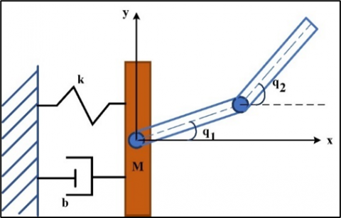
In this section, the dynamic modeling of a simple CBM is presented using Euler-Lagrange formulation. Figure 1 shows a planar 2-DOF robotic manipulator with 1-DOF compliant spring-damper base. The following assumptions are imposed within the current paper:
Figure 1. Schematics of a 3-DOF CBM
The whole dynamics for the coupled system are formulated as follows [15]
$m_t \ddot{x}+b \dot{x}+k x=a_1\left(\ddot{q}_1 s\left(q_1\right)+\dot{q}_1^2 c\left(q_1\right)\right)+a_2\left(\ddot{q}_2 s\left(q_2\right)+\dot{q}_2^2 c\left(q_2\right)\right)$ (1)
$J_1 \ddot{q}+a_2 d_1 c\left(q_2-q_1\right) \ddot{q}_2-a_1 s\left(q_1\right) \ddot{x}-a_2 d_1 s\left(q_2-q_1\right) \dot{q}_2^2=u_1-u_2$ (2)
$a_2 d_1 c\left(q_2-q_1\right) \ddot{q}_1+J_2 \ddot{q}_2-a_2 s\left(q_2\right) \ddot{x}+a_2 d_1 s\left(q_2-q_1\right) \dot{q}_1^2=u_2$ (3)
where, $\quad J_1=J_{z 1}+\frac{1}{4} m_1 d_1^2+m_2 d_2^2, J_2=J_{z 2}+\frac{1}{4} m_2 d_2^2, m_t=M+m_1+m_2, a_1=\left(0.5 m_1+m_2\right) d_1, a_2=$ $0.5 m_2 d_2$. The variable x is the relative position of base mass relative to equilibrium position, $\mathrm{s}()=.\sin ($.$) ,$ $\mathrm{c}()=.\cos (),. q_i$ is angular position of link $\mathrm{i}, J_{z i}$ is mass moment of inertia of link i about z -axis at CoM location, $d_i$ is the length of link i , and $u_i$ is control input applied at joint i to stabilize the robot motion. As we see, Eqs. (1)-(3) have three DoFs with only two control inputs and hence the system is underactuated.
Reformulation of the above equations in a matrix form results in
$\left[\begin{array}{ll}D_{11} & D_{12} \\ D_{21} & D_{22}\end{array}\right]\left[\begin{array}{l}\ddot{x} \\ \ddot{q}\end{array}\right]+\left[\begin{array}{ll}C_{11} & C_{12} \\ C_{21} & C_{22}\end{array}\right]\left[\begin{array}{l}\dot{x} \\ \dot{q}\end{array}\right]+\left[\begin{array}{c}K x \\ 0\end{array}\right]=\left[\begin{array}{c}0 \\ u\end{array}\right]$ (4)
where, $D_{11}=m_t$, $D_{12}=\left[a_1 s\left(q_1\right) \quad a_2 s\left(q_2\right)\right]$, $C_{11}=b, C_{12}=\left[\dot{q}_1 a_1 c\left(q_1\right) \quad \dot{q}_2 a_2 c\left(q_2\right)\right]$, $K=k$, $C_{21}=\left[\begin{array}{ll}0 & 0\end{array}\right]^T$, $C_{22}=\left[\begin{array}{cc}0 & a_2 d_1 c\left(q_2-q_1\right) \dot{q}_2 \\ a_2 d_1 c\left(q_2-q_1\right) \dot{q}_1 & 0\end{array}\right]$, $D_{21}=\left[\begin{array}{ll}-a_1 s\left(q_1\right) & -a_2 s\left(q_2\right)\end{array}\right]^T$, $D_{22}=\left[\begin{array}{cc}J_1 & a_2 d_1 c\left(q_2-q_1\right) \\ a_2 d_1 c\left(q_2-q_1\right) & J_2\end{array}\right]$.
From Eq. (4), we can get:
$\ddot{x}=-D_{11}^{-1}\left(D_{12} \ddot{q}+C_{11} \dot{x}+C_{12} \dot{q}+K x\right)$ (5)
Substituting Eq. (5) into Eq. (4), we obtain the following controllable dynamic system:
$\bar{D} \ddot{q}+\rho=u$ (6)
where, $\bar{D}=D_{11}-D_{12} D_{22}^{-1} D_{21}$, $\rho=C_{11} \dot{x}+C_{12} \dot{q}-D_{12} D_{22}^{-1}\left(C_{21} \dot{x}+C_{22} \dot{q}+K x\right)$.
The feedback linearization control strategy is to devise a nonlinear control law such that the resultant closed-loop system can be made linear. This way, a very intuitive controller, defined in Eq. (7), can be used [16-18]:
$u=\widehat{\bar{D}}\left(\ddot{q}_d+K_d\left(\dot{q}_d-\dot{q}\right)+K_p\left(q_d-q\right)\right)+\hat{\rho}+\sigma \operatorname{sgn}\left(B^T Q^T Z\right)$ (7)
where the symbol $\widehat{(.)}$ denotes estimated values, whereas the subscript (d) denotes the desired values. $K_d \in$ $R^{n \times n} K_p \in R^{n \times n}$ are matrices corresponding to the PD control gains, while $\sigma \in R^{n \times n}$ denotes robust sliding gain. The matrix $B$ is defined as
$B=\left[\begin{array}{c}0 \\ I_n\end{array}\right] \in R^{2 n \times n}$ (8)
with $I_n$ is a $n \times n$ identity matrix, and the vector z is given by:
$z=\left[\begin{array}{ll}e^T & \dot{e}^T\end{array}\right] \in R^{2 n}, e=q-q_d$ (9)
Besides, $Q=Q^T \in R^{2 n}$ is a symmetric positive definite matrix satisfying the Lyapunov equation:
$A^T Q+Q A=-P$ (10)
where, A is defined as $A=\left[\begin{array}{cc}0 & I_n \\ -K_p & -K_d\end{array}\right] \in R^{2 n \times 2 n}$ and $P=P^T \in R^{2 n \times 2 n}$ is also a symmetric positive definite matrix.Substituting Eq. (7) into Eq. (6) results in the following closed-loop dynamics:
$\ddot{e}+K_d \dot{e}+K_p e+\sigma \operatorname{sgn}\left(B^T Q^T z\right)=-\widehat{\bar{D}}^{-1}(\widetilde{D} \ddot{q}+\tilde{\rho})+\epsilon$ (11)
where, $\epsilon \in R^n$ represents the modeling/approximation errors. In fact, Eq. (11) describes a linear closed-loop system in the absence of the robust sliding term. However, the inclusion of this robust term introduces nonlinearity to the system. The application of the FAT allows formulation of the mass and nonlinear matrices/vectors as follows:
$\bar{D}=W_D^T \mu_D+\epsilon_D$ (12)
$\rho=W_\rho^T \mu_\rho+\epsilon_\rho$ (13)
where, $W_D \in R^{n l \times n}$ and $W_\rho \in R^{n l \times n}$ are weighting coefficients, $\mu_D \in R^{n l \times n}$ and $\mu_\rho \in R^{n l}$ are basisfunction matrices, with $l$ denoting the number of basis terms, and $\epsilon_{(.)}$is the related approximation error. Furthermore, in the same set of basis functions, the estimated values can be expressed:
$\widehat{\bar{D}}=\widehat{W}_D^T \mu_D$ (14)
$\hat{\rho}=\widehat{W}_\rho^T \mu_\rho$ (15)
The law of control in Eq. (7) can hence be rewritten as:
$u=\widehat{W}_D^T \mu_D\left(\ddot{q}_d+K_d\left(\dot{q}_d-\dot{q}\right)+K_p\left(q_d-q\right)\right)+\widehat{W}_\rho^T \mu_\rho+\sigma \operatorname{sgn}\left(B^T Q^T z\right)$ (16)
This implies that Eq. (16) should be substituted into Eq. (6) to get:
$\ddot{e}+K_d \dot{e}+K_p e+\sigma \operatorname{sgn}\left(B^T Q^T z\right)=-\widehat{W}_D^T \mu_D^{-1}\left(\widetilde{W}_D^T \mu_D \ddot{q}+\widetilde{W}_\rho^T \mu_\rho\right)+\epsilon$ (17)
Eq. (17) gives the following state-space representation:
$\dot{z}=A z-B\left\{\widehat{W}_D^T \mu_D^{-1}\left(\widetilde{W}_D^T \mu_D \ddot{q}+\widetilde{W}_\rho^T \mu_\rho\right)-\epsilon+\sigma \operatorname{sgn}\left(B^T Q^T z\right)\right\}$ (18)
To provide for the adaptation of the system behavior, the laws of adaptation are defined as follows:
$\dot{\vec{W}}_D=-\Lambda_D \mu_D \ddot{q}\left(z^T Q B \widehat{M}^{-1}\right)$ (19)
$\dot{\bar{W}}_\rho=-\Lambda_\rho \mu_\rho\left(z^T Q B \widehat{\bar{D}}^{-1}\right)$ (20)
where, $\Lambda_{(.)} \in R^{n l \times n l}$ is an adaptation matrix.
Remark 1. Because of their attractive numerical properties, Chebyshev polynomials were selected as approximators for the uncertainty:
Remark 2. This study used Chebyshev polynomials, but the FAT framework is flexible and can accommodate other types of bases such as:
These open possibilities for future work in hybrid or learned basis sets, particularly where the systems concerned benefit from greater nonlinearity or discontinuous types of operations.
These updates clarify the theoretical basis for using Chebyshev polynomials and prove that the approximation errors are considered in our control and stability design.
Theorem 1. The compliant base robot presented in (6) has dynamics that are Lyapunov-stable under the application of the control law with closed-loop dynamics along with the updating laws in (14)-(17).
Proof.
Let us choose the following Lyapunov-like function along the closed-loop dynamics in Eq. (18)
$v=\frac{1}{2} z^T P z+\frac{1}{2} \operatorname{tr}\left(\widetilde{W}_D^T \Lambda_D^{-1} \widetilde{W}_D+\widetilde{W}_\rho^T \Lambda_\rho^{-1} \widetilde{W}_\rho\right)$ (21)
Differentiating the above equation with respect to time gives:
$\dot{v}=-\frac{1}{2} z^T P z-z^T Q\left\{B \widehat{\bar{D}}^{-1}\left(\widetilde{W}_D^T \mu_D \ddot{q}+\widetilde{W}_\rho^T \mu_\rho\right)-B \epsilon+\sigma s g n\left(B^T Q^T z\right)\right\}-\operatorname{tr}\left(\widetilde{W}_D^T \Lambda_D^{-1} \dot{\bar{W}}_D\right)-\operatorname{tr}\left(\widetilde{W}_\rho^T \Lambda_\rho^{-1} \dot{\bar{W}}_\rho\right)$ (22)
Restating the Eq. (19) yields
$\begin{gathered}\dot{v}=-\frac{1}{2} z^T P z-\operatorname{tr}\left\{\widetilde{W}_D^T\left(\mu_D \ddot{q}\left(z^T Q B \widehat{M}^{-1}+\Lambda_D^{-1} \dot{\hat{W}}_D\right)\right)\right\}-\operatorname{tr}\left\{\widetilde{W}_\rho^T\left(\mu_\rho\left(z^T Q B \widehat{M}^{-1}+\Lambda_\rho^{-1} \dot{\widehat{W}}_\rho\right)\right)\right\}- \\ z^T Q B\left(-\epsilon+\sigma \operatorname{sgn}\left(B^T Q^T z\right)\right)\end{gathered}$ (23)
Substituting Eq. (19) into Eq. (23) cancels out the second and third terms, leading to
$\dot{v}=-\frac{1}{2} z^T P z-z^T Q B\left(-\epsilon+\sigma \operatorname{sgn}\left(B^T Q^T z\right)\right)=-\frac{1}{2} z^T P z+\aleph^T \epsilon-\sum_i \sigma_i\left|\aleph_i\right|$ (24)
with $\aleph=B^T Q^T Z$. Selecting the components $\sigma_i$ of the vector $\sigma$ as follows:
$\sigma_i \geq\left|\epsilon_i\right|+\beta_i$ (25)
where, $\beta_i$ is strictly a positive constant permits the following condition:
$\dot{v}=-\frac{1}{2} z^T P z-\sum_i \sigma_i\left|\aleph_i\right| \leq 0$. (26)
In this sense, Eq. (26) presented stable in the classical Lyapunov theory [19], as justification exists for choosing the sliding gain such that it dominates the approximation error. This reinstates that the derived conditions ensure uniform ultimate boundedness (UUB) of the tracking error by the standard Lyapunov theory.
The validity of the FAT-AFL controller using AFL is best seen in simulation experiments on a 3-DOF compliant-base robotic manipulator. A realistic simulation environment was built according to the physical parameters summarized in Table 1, which constitute those of lightweight, flexible robotic systems. The base stiffness was set to k = 800 N/m, which is of the order of compliant suspensions used in mobile platforms and aerial manipulators in the literature [20, 21]. The damping coefficient was set to c = 30 Ns/m, accounting for the passive viscous damping characteristics of industrial flexible fixtures and robotic suspension systems. The inertia and mass parameters represent a wide range of lightweight 2-DOF arms, such as segments of the UR5 robots (https://robodk.com/robot/Universal-Robots/UR5), surgical manipulators, or laboratory test rigs. There is nothing in the simulation setup to identify any commercial robot, but the parameter set captures the dynamics of compliant-supported robotic platforms realistically and can be re-tuned straightforwardly for stiffer or heavier systems.
Negligible approximation error is assumed in the FAT-AFL framework by utilizing enough orthogonal Chebyshev polynomial terms for function approximation (l = 15). Hence, the robust sliding term is considered not necessary in simulation. Performance brought from control evaluated in the state in which the manipulator was released from static with joint angles positioned to π/3 rads, allowing the system to undergo transitory oscillation before settling. Control gains Kp and Kd were chosen initially by second pole-place methods that identify with a damping ratio ζ=0.8 and settling time less than 4 seconds. Gains were increased gradually from zero up to the point of instability, after which they were halved, a technique commonly used in iterative controller tuning. The final gains used were Kp = diag(180,170) and Kd = diag(60,55), with adaptation gains Λρ= diag(100,100,...,100) ∈ R30×30. The weight coefficient matrix for the approximator was initialized to zero.
Table 1. Physical parameters used in simulation [15]
|
Parameter |
Value |
|
M |
3 kg |
|
$m_1$ |
0.4 kg |
|
$m_2$ |
0.2 kg |
|
$d_1$ |
0.15 m |
|
$d_2$ |
0.15 m |
|
c |
30 Ns/m |
|
k |
800 N/m |
|
$J_{z 1}$ |
7.5 × 10⁻⁴ kg.m2 |
|
$J_{z 2}$ |
3.75 × 10⁻⁴ kg.m2 |
The FAT-AFL controller was compared to two classical approaches: the PD + I structure joint-wise for PID control and a Sliding Mode Control (SMC) approach comprising both equivalent and discontinuous control terms. All controllers are tested with identical initial conditions. The results in summary, as given in Table 2, show the superiority with respect to overshoot, settling time, steady-state error, maximum torque applied, and energy consumption control of the FAT-AFL controller test case.
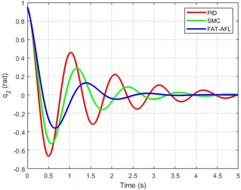
In contrast to PID, which had slow adaptation, and SMC, which introduced chattering on the control signal, FAT-AFL provided smooth, accurate response exceedingly robust to model uncertainties and used very low control effort. The controller successfully guided the manipulator in a slew from an upright position across 3 radians in a time of about 3.7 seconds without giving rise to residual vibrations (Figures 2-4). The control inputs were kept below 0.01 Nm for u₁ and 0.003 Nm for u₂, confirming the ability to control motion with a minimum of force application (Figures 5 and 6). In sum, the FAT-AFL controller:
Figure 2. The link angle $q_1$ response under three control techniques
Table 2. Comparison with performance metrics
|
Controller |
Overshoot (%) |
Settling Time (s) |
Steady-State Error |
Max Torque (Nm) |
Control Energy |
|
PID |
11.2 |
4.8 |
0.03 rad |
0.012 |
High |
|
SMC |
6.4 |
3.9 |
0.01 rad |
0.015 (chatter) |
Moderate |
|
FAT-AFL |
3.2 |
3.7 |
<0.005 rad |
0.004 |
Low |
Figure 3. The link angle $q_2$ response under three control techniques
Figure 4. The base oscillations under three control techniques
Figure 5. Control input $u_1$ under three control techniques
Figure 6. Control input $u_2$ under three control techniques
This investigation intended an AFL control approach with a FAT and a robust sliding compensator for control challenges posed by compliant base robotic manipulators. The rigid manipulator with the compliant base was modeled with high fidelity using the Euler-Lagrange formulation, while treating base dynamics as external disturbances. The use of Chebyshev polynomial basis functions in the FAT scheme was justified by their minimax property and computational efficiency. Therefore, the controller compensates for disturbances by robustification and adaptive learning, thus providing accurate tracking and vibration suppression. The stability of the total system and the convergence of the adaptive laws were then theoretically verified using the Lyapunov theory. The efficacy of the proposed control strategy is demonstrated through simulation studies on a 3-DOF flexible base manipulator that results in a very fast response coupled with damped oscillations. Thus, it can be concluded that this method has great potential for improving the performance of compliant robotic systems in dynamic and complex environments.
In terms of future perspectives, research will extend the proposed control framework to higher degree-of-freedom (DOF) manipulators, as well as experimental validation on physical robotic platforms. It is important to consider sensor noise, actuator saturation, and time delay effects to evaluate the real-world robustness. The suite of learning-based control algorithms (like reinforcement learning or neural network optimization) may further account for the dynamic and uncertain nature-of-context changes with regards to adaptability. Another area with promise is cooperation among robot-robot systems equipped with compliant bases.
|
$x$ |
the relative position of the base mass relative to equilibrium position. |
|
$q_i$ |
angular position of link i |
|
$J_{z i}$ |
mass moment of inertia of link i about z-axis at CoM location |
|
$d_i$ |
the length of link i |
|
$u_i$ |
control input applied at joint i |
|
$K_p$ |
the proportional gain matrix, $\in R^{n \times n}$ |
|
$K_d$ |
the derivative gain matrix, $\in R^{n \times n}$ |
|
$W_{(.)}$ |
the weighting coefficient matrix, $\in R^{n l \times n}$ |
|
$\mu_{(.)}$ |
the orthogonal basis function matrix/vector depending on the dimension of the estimated uncertainty |
|
$v$ |
The Lyapunov-like function |
[1] Chong, N.Y., Yokoi, K., Oh, S.R., Tanie, K. (1997). Position control of collision-tolerant passive mobile manipulator with base suspension characteristics. In Proceedings of International Conference on Robotics and Automation, Albuquerque, NM, USA, pp. 594-599. https://doi.org/10.1109/ROBOT.1997.620101
[2] Lew, J.Y., Moon, S.M. (1999). Acceleration feedback control of compliant base manipulators. In Proceedings of the 1999 American Control Conference (Cat. No. 99CH36251), San Diego, CA, USA, pp. 1955-1959. https://doi.org/10.1109/ACC.1999.786203
[3] Yang, B.J., Calise, A.J., Craig, J.I. (2007). Adaptive output feedback control of a flexible base manipulator. Journal of Guidance, Control, and Dynamics, 30(4): 1068-1080. https://doi.org/10.2514/1.23707
[4] Yoshida, K., Nenchev, D.N., Uchiyama, M. (1996). Moving base robotics and reaction management control. In Robotics Research: The Seventh International Symposium, pp. 100-109. Springer. https://doi.org/10.1007/978-1-4471-1021-7_11
[5] Vijayan, R., De Stefano, M., Dietrich, A., Ott, C. (2021). Unified control of an orbital manipulator for the approach and grasping of a free-floating satellite. IEEE/ASME Transactions on Mechatronics, 26(6): 2904-2915. https://doi.org/10.1109/TMECH.2021.3081444
[6] Zhang, H., Li, S., Zhang, L. (2022). Fractional-order sliding mode control for free-floating space manipulators with disturbance and input saturation. International Journal of Adaptive Control and Signal Processing, 36(12): 1973-1988. https://doi.org/10.1002/rnc.7826
[7] Liu, Y., Luo, K., Tian, Q., Hu, H. (2025). Nonlinear dynamics design for in-space assembly motion of manipulators on flexible base structures. Nonlinear Dynamics, 113: 9485-9507. https://doi.org/10.1007/s11071-024-10588-w
[8] Sun, E., Camacho-Arreguin, J., Zhou, J., Liebenschutz-Jones, M., Zeng, T., Keedwell, M., Norton, A., Axinte, D., Mohammad, A. (2025). Macro-mini collaborative manipulator system for welding in confined environments. Robotics and Computer-Integrated Manufacturing, 80: 102517. https://doi.org/10.1016/j.rcim.2025.102517
[9] Tang, Y. (2025). Research on boundary control of vehicle-mounted flexible manipulator based on partial differential equations. PLOS ONE, 20(1): e0317012. https://doi.org/10.1371/journal.pone.0317012
[10] Nenchev, D.N., Yoshida, K., Vichitkulsawat, P., Uchiyama, M. (1999). Reaction null-space control of flexible structure mounted manipulator systems. IEEE Transactions on Robotics and Automation, 15(6): 1011-1023. https://doi.org/10.1109/70.817666
[11] Ott, C., Albu-Schaffer, A., Hirzinger, G. (2006). A cartesian compliance controller for a manipulator mounted on a flexible structure. In 2006 IEEE/RSJ International Conference on Intelligent Robots and Systems, Beijing, China, pp. 4502-4508. https://doi.org/10.1109/IROS.2006.282539
[12] Lin, J., Huang, Z.Z. (2007). A hierarchical fuzzy approach to supervisory control of robot manipulators with oscillatory bases. Mechatronics, 17(10): 589-600. https://doi.org/10.1016/j.mechatronics.2007.07.008
[13] Casella, F., Locatelli, A., Schiavoni, N. (2000). Modelling and control for vibration suppression in a large flexible structure with jet thrusters and piezoactuators. In Proceedings of the 39th IEEE Conference on Decision and Control (Cat. No. 00CH37187), Sydney, NSW, Australia, pp. 4491-4499. https://doi.org/10.1109/CDC.2001.914616
[14] Wie, B. (1998). Space Vehicle Dynamics and Control. AIAA Educational Series.
[15] Reyhanoglu, M., Hoffman, D. (2017). Finite-time control of a compliant base robot manipulator. In 2017 11th Asian Control Conference (ASCC), Gold Coast, QLD, Australia, pp. 1335-1340. https://doi.org/10.1109/ASCC.2017.8287365
[16] Al-Shuka, H.F.N., Corves, B. (2023). Function Approximation Technique (FAT)-based adaptive feedback linearization control for nonlinear aeroelastic wing models considering different actuation scenarios. Mathematical Models and Computer Simulations, 15(2): 152-166. https://doi.org/10.1134/S2070048223010106
[17] Al-Shuka, H.F., Abbas, E. (2022). Function Approximation Technique (FAT)-based nonlinear control strategies for smart thin plates with cubic nonlinearities. FME Transaction, 50(1): 168-180. https://dx.doi.org/10.5937/fme2201168A
[18] Kaleel, A.H., Al-Shuka, H.F.N., Hussein, O. (2021). Adaptive approximation-based feedback linearization control for a nonlinear smart thin plate. International Journal of Mechanical Engineering and Robotics Research, 10(8): 458-463. https://doi.org/10.18178/ijmerr.10.8.458-463
[19] Slotine, J.J.E., Li, W. (1991). Applied Nonlinear Control. Englewood Cliffs, NJ, USA: Prentice Hall.
[20] Casella, C., Ceccarelli, M., Carbone, G. (2002). Design and simulation of a light compliant suspension system for service robots. In Proceedings of 9th International Conference. Advanced Robotics (ICAR), Tokyo, Japan, pp. 199-204.
[21] Lew, J.Y., Moon, Y.M. (1999). Vibration isolation with a compliant parallel mechanism and a passive damper. Journal of Robotic Systems, 16(6): 353-363.