Parameters Identification of Induction Motor with Hybrid Metaheuristic Algorithm: Equilibrium Slime Mould

Modeling the IM is necessary to estimate its parameters. Therefore, a model closely matching the real IM was used, as validated in the frequency domain using the modified Park model SSFR [27]. Nonlinear mathematical equations were used for modeling an IM with reference to the rotor (d, q) axes.

$\left( \begin{align}  & {{u}_{ds}}={{R}_{s}}{{I}_{ds}}+\frac{d{{\Phi }_{ds}}}{dt}-{{\omega }_{r}}{{\Phi }_{qs}} \\ & {{u}_{qs}}={{R}_{s}}{{I}_{qs}}+\frac{d{{\Phi }_{qs}}}{dt}+{{\omega }_{r}}{{\Phi }_{ds}} \\ & 0={{R}_{r}}{{I}_{dr}}+\frac{d{{\Phi }_{dr}}}{dt} \\ & 0={{R}_{r}}{{I}_{qr}}+\frac{d{{\Phi }_{qr}}}{dt} \\\end{align} \right)$                  (1)

with

$\left( \begin{align}  & {{\Phi }_{ds}}=\left( M+{{L}_{s}} \right){{I}_{ds}}+M{{I}_{dr}} \\ & {{\Phi }_{qs}}=\left( M+{{L}_{s}} \right){{I}_{qs}}+M{{I}_{qr}} \\ & {{\Phi }_{dr}}=\left( M+{{L}_{r}} \right){{I}_{dr}}+M\left( {{I}_{ds}}+{{I}_{dr}} \right) \\ & {{\Phi }_{qr}}=\left( M+{{L}_{r}} \right){{I}_{qr}}+M\left( {{I}_{qs}}+{{I}_{qr}} \right) \\\end{align} \right)$              (2)

Then the machine's nonlinear equations can be written as follows:

$\left( \begin{align}  & {{u}_{ds}}={{R}_{s}}{{I}_{ds}}+\left( M+{{L}_{s}} \right)\frac{d{{I}_{ds}}}{dt}+M\frac{d{{I}_{dr}}}{dt}-{{\omega }_{r}}\left( M+{{L}_{s}} \right){{I}_{qs}}-{{\omega }_{r}}M{{I}_{qr}} \\  & {{u}_{qs}}={{R}_{s}}{{I}_{qs}}+\left( M+{{L}_{s}} \right)\frac{d{{I}_{qs}}}{dt}+M\frac{d{{I}_{qr}}}{dt}-{{\omega }_{r}}\left( M+{{L}_{s}} \right){{I}_{ds}}+{{\omega }_{r}}M{{I}_{qr}} \\ & 0={{R}_{r}}{{I}_{dr}}+\left( M+{{L}_{r}} \right)\frac{d{{I}_{dr}}}{dt}+M\frac{d{{I}_{ds}}}{dt} \\ & 0={{R}_{r}}{{I}_{qr}}+\left( M+{{L}_{r}} \right)\frac{d{{I}_{qr}}}{dt}+M\frac{d{{I}_{qs}}}{dt} \\\end{align} \right.$              (3)

where, $R_rR_s$ rotor resistance and stator resistance, $L_sL_r$ stator inductance and rotor inductance.

It can be done to complete the motor's differential equations with the movement equations expressed by (4) and (5).

$j\frac{d{{\omega }_{r}}}{dt}={{C}_{em}}-{{C}_{r}}-F{{\omega }_{r}}$                     (4)

${{C}_{em}}=\frac{3}{2}M\left( {{I}_{qs}}{{I}_{dr}}-{{I}_{ds}}{{I}_{qr}} \right)$                   (5)

where, $j$ represents the moment of inertia of the IM under study, $C_{em}$ its electromagnetic torque, $F$ its viscous friction, $C_r$ its load torque.

Figure 1 illustrates the mathematical model of a three-phase IM in the dq reference frame. The model was developed using the Simulink environment and is based on the dynamic equations of the motor transformed into the rotating reference frame. The three-phase voltages (Va, Vb, Vc) are converted into dq components using the Park transformation, which simplifies the analysis by reducing the system to two dimensions. The model includes both the electrical circuits of the motor and the mechanical equations that relate the generated torque to the rotor dynamics. A small simulation time step (0.0001 s) is used to ensure high accuracy in the transient response analysis.

1.png

Figure 1. Simulink block diagram of the IM [27]

2.1 SMA

SMA is a new algorithm based on metaheuristics proposed by Li et al. [28] Slime mold is a living organism that thrives in cold and humid environments. It spreads and reproduces in areas with abundant food. Slime mold moves toward food by detecting its scent, thereby spreading and enveloping itself around the food source. A mathematical model corresponding to this natural phenomenon was simulated using three different equations.

$\overrightarrow{{{x}_{\left( i+1 \right)}}}=\left\{ \begin{align}  & rand.\left( ub-lb \right)+lb \\ & \overrightarrow{{{x}_{B\left( i+1 \right)}}}+\overrightarrow{va}.\left( \overrightarrow{w.}\overrightarrow{{{x}_{f\left( i \right)}}}-\overrightarrow{{{x}_{j\left( i \right)}}} \right) \\ & \overrightarrow{vb}.\overrightarrow{{{x}_{\left( i \right)}}} \\\end{align} \right.\begin{matrix}   rand\prec z  \\   r\prec q  \\   r\ge q  \\\end{matrix}$                    (6)

where, $i$ is the number of iterations, $\overrightarrow{x_{(i+1)}}$ represents the position of the new mold particle, $\overrightarrow{x_{B}}$ is the location with the currently identified high concentration of food odors, $lb$ it symbolizes the lower limits, $ub$ it symbolizes the upper limits, $\overrightarrow{x_{f(i)}}$ and $\overrightarrow{x_{j(i)}}$ it is two randomly selected individual mold locations.  $rand$ and $r$ is a variable number from 0 to 1, $\overrightarrow{va}$ is a variable number in the interval [-d,d], $\overrightarrow{vb}$ decreases linearly from 1 to 0, d is defined as follows:

$d=\arctan h\left( i-\frac{i}{\max \_i} \right)$                 (7)

where, $max\_i$ is the number of maximal iterations. $\overrightarrow{w}$ is the transfer coefficient from the mold particle to the food location, and this factor changes from particle to particle depending on the value of the target function. $\overrightarrow{w}$ is defined on:

$\overrightarrow{{{w}_{\left( SIdx\left( n \right) \right)}}}=\left\{ \begin{align}  & 1+r.\log \left( \frac{Bf-{{s}_{\left( n \right)}}}{Bf-wf}+1 \right) \\ & 1-r.\log \left( \frac{Bf-{{s}_{\left( n \right)}}}{Bf-wf}+1 \right) \\\end{align} \right.\begin{matrix}   n\prec \frac{m}{2}  \\   n\succ \frac{m}{2}  \\\end{matrix}$                  (8)

where, $n=1,2,...,m$

$m$ is the number of mold particles, $r$ is a random numerical variable between 0 and 1, $Bf$ represents the best value of the objective function for each iteration, $wf$ represents the worst value of the objective function, $s_{(n)}$ represents the value of the objective function for each mold particle, $SId_x$ represents the sequence of sorted objective function values.

$q=\tanh \left| {{s}_{\left( n \right)}}-FI \right|$                 (9)

where, $FI$ represents the optimal value of the objective function calculated over all iterations. The transmission and spread of slime mold is based on three different equations:

When $rand \prec z$, one equation is used.

When $r \prec q$, another equation is used.

When $r \geq q$, a third equation is used.

It is set to z= [0.03 – 0.06] range in the SMA.

2.2 Equilibrium optimizer algorithm

The EO algorithm is inspired by modern physics and is based on the principle of balancing mass and volume, as proposed in recent research [29]. The concept is described by the following equation.

$\overrightarrow{{{c}_{1}}}=\overrightarrow{{{c}_{eq}}}+\overrightarrow{F}\left( \overrightarrow{{{c}_{0}}}-\overrightarrow{{{c}_{eq}}} \right)+\left( 1-\overrightarrow{F} \right)\frac{\overrightarrow{j}}{\left( \overrightarrow{\gamma .}v \right)}$                  (10)

where, $\overrightarrow{c_1}$ represents the updated solution, $\overrightarrow{c_0}$ represents the preceding solution, $\overrightarrow{c_{eq}}$ indicates the best solution, $\overrightarrow{F}$ is a coefficient applied to weigh local and global search efforts. $\overrightarrow{j}$ represents the density development rate in the test volume, $\gamma$ is the variable of probability numbers in [0, 1]. v=1 indicates unity of volume. There are five candidate solutions in the balance basin. The four most intriguing solutions discovered thus far are listed below, with the second representing the central location (average concentration) of these four contender solutions, as illustrated:

$\overrightarrow{{{c}_{eq,pool}}}=\left\{ \overrightarrow{{{c}_{eq,1}}},\overrightarrow{{{c}_{eq,2}}},\overrightarrow{{{c}_{eq,3}}},\overrightarrow{{{c}_{eq,4}}},\overrightarrow{{{c}_{eq,ave,}}} \right\}$

$\overrightarrow{F}={{A}_{1}}.siqn\left( \overrightarrow{r}-0.5 \right).\left( {{e}^{\overrightarrow{\gamma }{{T}_{1}}}}-1 \right)$

${{T}_{1}}={{\left( i-\frac{i}{\max \_i} \right)}^{\left( {{A}_{2.}}.\frac{t}{\max \_i} \right)}}$                   (11)

where, $A_1 \in$[1,2] and $A_2 \in$[1,2] represent the fixed global search force coefficient. The larger $A_1 \in$[1,2] the greater the exploration capacity and the lower the exploitation capacity, and vice versa. The $\overrightarrow{J}$ value is expressed as:

$\overrightarrow{J}=\left( \begin{align}  & 0.5{{r}_{1}}\left( \overrightarrow{{{c}_{eq}}}-\overrightarrow{\gamma }\overrightarrow{c} \right)\overrightarrow{F} \\ &0\\\end{align}\right.\begin{matrix}   {{r}_{2}}\ge jp  \\   {{r}_{2}}\le jp  \\\end{matrix}$                   (12)

where, $r_1$ and $r_2$ are probability numbers in [0,1] and where $jp$=0.5 is the random probability of generation.

2.3 Proposed a new hybrid metaheuristic algorithm EOSMA, for IM parameters identification

The EOSMA algorithm is a recently proposed method representing a hybrid of the SMA and EO algorithms. This hybrid algorithm was developed to enhance the performance of metaheuristic solutions, aiming to achieve high convergence speed and solution accuracy. By integrating the strengths of SMA and EO, the algorithm provides a robust approach for finding optimal solutions. It employs strategies that accelerate the convergence process, enabling it to reach optimal solutions in a shorter time while maintaining high accuracy in solving complex problems. Additionally, EOSMA combines global search mechanisms (exploration) with focused search mechanisms (exploitation), ensuring comprehensive coverage of the search space and improving solution quality. The algorithm operates using mathematical equations derived from the unique features of SMA and EO, performing heuristic searches through iterative steps where solutions are gradually refined through the interaction of both algorithms’ components [23].

$\overrightarrow{{{x}_{\left( i+1 \right)}}}=\left\{ \begin{align}  & \overrightarrow{{{x}_{eq\left( i \right)}}}+\left( \overrightarrow{{{x}_{\left( i \right)}}}-\overrightarrow{{{x}_{eq\left( i \right)}}} \right).\overrightarrow{F}+\left( 1-\overrightarrow{F} \right)\frac{\overrightarrow{j}}{\left( \overrightarrow{\gamma .}v \right)} \\ & \overrightarrow{{{x}_{eq,1\left( i \right)}}}+\overrightarrow{va}.\left( \overrightarrow{w.}\overrightarrow{{{x}_{f\left( i \right)}}}-\overrightarrow{{{x}_{j\left( i \right)}}} \right) \\ & \overrightarrow{{{x}_{\left( i \right)}}}+\overrightarrow{vb}.\overrightarrow{{{x}_{\left( i \right)}}} \\\end{align} \right.\begin{matrix}   rand\prec z  \\   r\prec q  \\   r\ge q  \\\end{matrix}$                   (13)

where, $\overrightarrow{x_{(i)}}$ is the location of the equilibrium point, $\overrightarrow{x_{eq(i)}}$ is a solution chosen at random from the equilibrium pool with equal probability, $\overrightarrow{x_{eq,1(i)}}$ is the best solution in the equilibrium pool, the best position found so far, and z is an empirical value obtained through experiments, r is a random number vector in the range [0,1]. The H vector is defined by:

${{H}_{a,y}}=\left( \begin{align}  & 1 \\ & 0 \\\end{align} \right.\begin{matrix}   rand\prec k  \\   rand\ge k  \\\end{matrix}$

$\begin{align}  & a=1,2,...,pop. \\ & y=1,2,...,\operatorname{var}. \\\end{align}$                   (14)

where, $a$ is population size, y indicates the number of dimensions, k=0.2 is an settable variable, to ensure that the searches are not spoiled, the limits of the search operator are updated by Eq. (15) each time the location is updated:

$\overrightarrow{x_{a, y(i+1)}}=\left\{\begin{array}{lr}\frac{\left(x_{a, y(i)}+U B\right)}{2} & \overrightarrow{x_{a, y(i+1)}}\succ U B \\ \frac{\left(x_{a, y(i)}+U B\right)}{2} & \overrightarrow{x_{a, y(i+1)}}\prec U B \\ \frac{\text { others }}{x_{a, y(i+1)}} &others \end{array}\right.$                   (15)

$UB$ symbolizes the upper limits.

Table 1 shows the organizational structure for the programming algorithm EOSMA, which is a hybrid metaheuristic algorithm that combines the two algorithms, EO and SMA.

Table 1. Organizational structure for the programming algorithm EOSMA

Table 5. Identified parameters of IM with EO SMA EOSMA algorithms

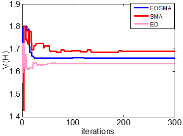
Figure 4 presents the progression of the objective function over successive iterations for the EOSMA, EO, and SMA algorithms. It is evident that EOSMA achieves convergence by approximately the 40th iteration, compared to the EO algorithm, which converges around the 60th iteration, and the SMA algorithm, which converges by the 80th iteration. These results clearly indicate that EOSMA not only converges more rapidly but also achieves superior objective function values. This comparison underscores the effectiveness of EOSMA in terms of both convergence speed and solution quality. The hybridization of SMA and EO successfully combines the strengths of both algorithms—balancing exploration and exploitation—to produce more accurate and efficient optimization outcomes. From a computational standpoint, while EOSMA may incur a slightly higher processing cost due to the integration of two algorithmic frameworks, its accelerated convergence often offsets this overhead. In practice, the algorithm requires fewer iterations to reach optimal or near-optimal solutions, which can lead to significant time savings overall. Therefore, despite its marginally higher computational demand, EOSMA proves to be a robust and efficient choice, particularly for applications that demand high precision and rapid convergence.

4.png

Figure 4. Objective function

5.png

Figure 5. Stator phase resistance

6.png

Figure 6. Stator inductance

7.png

Figure 7. Rotor inductance

8.png

Figure 8. Rotor phase resistance

9.png

Figure 9. Mutual inductance

10.png

Figure 10. J moment of inertia of the IM

11.png

Figure 11. Coefficient of friction f

Figures 5-11 show the changes in IM parameters as a function of iterations. EOSMA, EO, and SMA search for IM parameters in the research space indicated in Table 4. At the beginning of the iteration, the algorithms provide random parameters, and the error rate of the parameters is large. After 80 iterations, the parameters begin to converge to the correct results. After the research is completed. We conclude that algorithm EOSMA obtained better and more accurate results because the objective function EOSMA is minimized (objective function EOSMA: 0.8).

12.png

Figure 12. Experimental speed

13.png

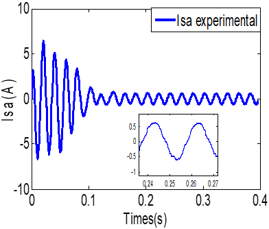
Figure 13. Experimental stator current

Figures 12 and 13 illustrate the evolution of angular velocity and current intensity over a short time interval. The upper curve shows a rapid increase in angular velocity, stabilizing around 300 rad/s, indicating efficient dynamic system performance. The lower curve displays damped oscillations in the current signal, reflecting transient behavior due to electromagnetic interactions. These results contribute to understanding the system’s dynamic response and evaluating its accuracy.

14.png

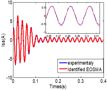
Figure 14. IM stator current obtained from simulation and experimental with identified parameters based on EOSMA

15.png

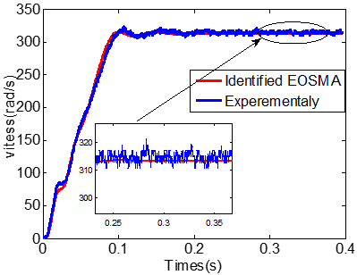
Figure 15. IM speed obtained from simulation and experimental with identified parameters based EOSMA

Figure 14 shows the difference (error) between the current intensity obtained from the mathematical model of the IM and the experimental model of the IM. Likewise, Figure 15 shows the difference (error) between the speed obtained from the mathematical model of the IM and the experimental model of the IM. These results obtained with precision prove by evidence the usefulness and validation of the EOSMA algorithm for the identification of the IM parameters.