Noureddine Fares*![]() | Chouaib Souaidia
| Chouaib Souaidia![]() | Tawfik Thelaidjia
| Tawfik Thelaidjia![]()
© 2025 The authors. This article is published by IIETA and is licensed under the CC BY 4.0 license (http://creativecommons.org/licenses/by/4.0/).
OPEN ACCESS
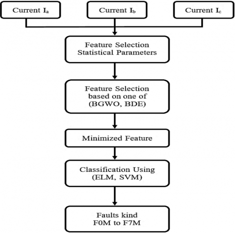
This study provides an innovative structure to diagnose the malfunction of the grid-connected photovoltaic energy systems (GPV), depending on the two bilateral improvements: the gray wolf (BGWO) and the differential development (BDE), as well as choosing the properties and classification of automatic learning (ELM and SVM). The proposed methodology relies on real data and includes the following steps: Firstly, we extract statistical parameters from all data sources. Second, the BGWO and BDE algorithms are used separately to choose the properties and reduce their number. Finally, the Extreme Learning Machine (ELM) and the support machine (SVM) are employed to identify seven main breakdowns, namely: nonhomogeneous partial shading, inverter fault, feedback sensor fault, MPPT controller fault, grid anomaly, open circuit in PV array, and boost converter controller fault. The results obtained indicate that the Extreme Learning Machine (ELM) algorithm associated with the BGWO chosen algorithm provides an optimal input vector that detects faults with high accuracy (99.16%) compared to other approaches.
binary grey wolf optimization (BGWO), binary differential evolution (BDE), extreme learning machine (ELM), support vector machine (SVM), advanced monitoring, grid-connected PV systems, maximum power point tracking (MPPT)
Solar energy costs should continue to decrease due to technological progress. Enhancing the durability and operational reliability of PV modules is a key aspect in driving down the cost of photovoltaic (PV) systems [1]. Nevertheless, these systems remain susceptible to various anomalies, which must be swiftly identified to prevent divergence from optimal operating conditions [2].
To ensure long-term performance and efficiency, it is essential to implement proactive measures that preserve system reliability and safety. This proactive approach is critical to aligning with the protection standards outlined by the International Electrotechnical Commission (IEC) [3, 4]. Timely identification of faults is vital for sustaining energy output, maintaining nominal operating conditions, and delivering consistent power quality [5]. Fast fault detection (FD) mechanisms not only improve the availability rate of PV systems by minimizing downtime but also support compliance with grid regulation requirements.
Effective system monitoring enhances energy output, reduces maintenance expenses, and improves the overall return on investment throughout the system's life cycle [6, 7]. In addition to their non-linear and variable characteristics in time and their high dependence on environmental factors (such as temperature and irradiance), PV systems naturally inherit properties specific to electrical systems. They thus have a very fast dynamic, with sudden changes even faster. This underscores the necessity for regular and diverse measurements utilizing sensors to monitor the grid-connected photovoltaic system (GPV) and the dynamics of its failures. However, this requirement generates a bottleneck in terms of computer processing. Detection of defects linked to sensors in GPV systems [8]. The researchers also proposed an optimal configuration for positioning current and voltage sensors, aiming to minimize the increased costs linked to redundant measurement devices. Additionally, a sensor-based analysis to facilitate the detection of partial shading conditions [9].
These methods rely on monitoring localized signals, such as the current in the PV string, which are then compared to established reference models to identify localized faults [10, 11]. An in-depth assessment of metaheuristic tools is used [12]. Methods for identifying faults in photovoltaic systems often rely on mathematical or analytical frameworks, including the use of state observers [13], While parameter identification techniques [12] and impedance-based models [14] have yielded positive results in simulations, their use in practical settings is often hindered by their sensitivity to measurement noise and uncertainties within the models. Analytical methods often fall short in addressing the inherent complexity of real-world photovoltaic (PV) systems, which are difficult to represent accurately using closed-form mathematical models, especially under varying conditions. In contrast, artificial intelligence (AI) has emerged as a powerful and versatile tool, with widespread applications across numerous domains—including medicine, astronomy, engineering, robotics, speech recognition, natural language processing, and behavioral sciences. In the field of photovoltaics, AI techniques have become particularly valuable, notably for forecasting and predictive analysis tasks [15]. For data-driven fault detection in photovoltaic (PV) systems, various techniques can be employed, including statistical analyses and machine learning approaches, both of which are well-suited for addressing complex and nonlinear challenges. Among the artificial intelligence methods commonly applied to PV systems are artificial neural networks [16], fuzzy logic systems [17], decision tree algorithms, and the k-nearest neighbors (K-NN) method [18]. The most widely adopted deep learning models for identifying and classifying faults in photovoltaic systems include convolutional neural networks (CNNs), long short-term memory networks (LSTMs), recurrent neural networks (RNNs), generative adversarial networks (GANs), Boltzmann machines, and auto encoders [19]. An auto encoder is a type of neural network that learns to compress input data into a lower-dimensional representation and then reconstruct the original input from this encoded format [20]. The output produced by the autoencoder is fed back as its own input, allowing the network to learn representative features by minimizing the reconstruction error [21].
A full assessment of issues connected to the identification of faults and protection in solar systems [22], where defects were grouped into three categories: physical, electric, and environmental. The continuous protection devices (DC) attempt to guard against overcurrent’s, grounding problems, and electric arcs [23]. Yet, these protections may fail to detect certain module-level issues due to factors such as (i) weak fault currents, (ii) interference from MPPT (Maximum Power Point Tracking) regulators, and (iii) the non-linear and irradiance-dependent behavior of PV modules [22]. Undetected DC-side faults can significantly degrade performance and, in severe cases, cause fires despite existing safety mechanisms [24]. An investigation of AC micro grid protection strategies [25], where solutions are grouped into three categories: grid-tied protection, islanded mode protection, and hybrid approaches. Additionally, as digital transformation progresses, new cyber threats present complex challenges for identifying and diagnosing cyberattacks in large-scale power systems [26]. This study focuses on analyzing the three aforementioned challenges (I, II, III) in grid-connected photovoltaic (GPV) systems. Traditional diagnostic methods often struggle with the time-varying, non-linear nature of these systems and the masking effects introduced by MPPT controllers. Advanced diagnostic tools are therefore necessary, particularly under conditions where MPPT algorithms obscure fault symptoms, especially those with low current signatures.
Identifying issues in solar power systems that utilize an MPPT controller frequently necessitates the use of sophisticated fault diagnosis (FD) techniques. Sophisticated Maximum Power Point Tracking (MPPT) techniques, such as a dynamic leader-based collective intelligence method [27] and the MSS algorithm [28], have proven to be fast and efficient in reducing power losses under partial shading conditions. However, these very strengths complicate defect detection for two main reasons: MPPT algorithms tend to mask the signs of faults, particularly those involving low current, and the wide variety of potential defects is made even more complex by the operation of MPPT controllers. For a recent overview of MPPT algorithms, see the studys [29, 22], discusses the detrimental effects of MPPT controllers on fault diagnosis in solar systems.
Addressing the challenges posed by MPPT controllers in fault detection, this study introduces a novel Fault Diagnosis (FD) method. This technique utilizes the Extreme Learning Machine (ELM) and Support Vector Machine (SVM), enhanced by Binary Grey Wolf Optimization (BGWO) and Binary Differential Evolution (BDE) for feature selection, to identify faults in grid-connected PV systems operating under MPPT mode. The research employs actual failure data obtained from a real GPV system utilizing PSO-based MPPT controllers, with the experimental datasets provided by the study [30].
This paper is structured as follows: Section 2 introduces the Grid-Connected Photovoltaic (GPV) system, highlighting its dynamic and non-linear nature, along with the specific faults examined. Sections 3 and 4 detail the primary contribution: an ELM and SVM-based learning machine for detecting seven faults in grid-connected PV systems under MPPT control. Section 5 explains the extraction of five statistical features from data representing different fault scenarios, which are then used as input for training and testing the ELM and SVM to classify system states. Section 6 describes the use of BGWO and BDE for input vector optimization. Section 7 presents the application of ELM and SVM to detect the seven fault types. Section 8 then presents the findings, demonstrating a fault classification rate of up to 99.16%. Finally, Section 9 summarizes the key conclusions and offers recommendations.
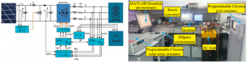
The grid-connected photovoltaic system examined in this study is implemented as shown in Figure 1. This section focuses on the theoretical aspects of GPV systems, particularly their non-linear and time-varying behavior. This behavior can be theoretically explained through the ideal diode model, which describes the connection between the system's output voltage $V_{P V}$ and current $I_{P V}$.
$\begin{gathered}I_{P V}=I_{\text {irr }}-I_0\left[exp \left(\frac{V_{P V}+R_S I_{P V}}{V_{ {therm }} n}\right)-1\right] \\ -\frac{V_{P V}+R_S I_{P V}}{R_{s h}}\end{gathered}$ (1)
Figure 1. GPV system implementation [32]
The electrical behavior of a solar cell can be described by several key parameters. In the context of an ideal diode model, '$n$' represents the ideality factor of the cell, a dimensionless parameter that characterizes the deviation of the diode's behavior from the ideal case. '$V_{\text {therm }}=k T / q$' denotes the thermal voltage of the cell, a voltage scale that depends on temperature. This thermal voltage is determined by the Boltzmann constant 'k' and the junction temperature 'T', as well as the electronic charge 'q'. Finally, '$R_{s h}$, $R_s$' indicates the shunt resistance and the series resistance, which represent losses within the cell due to leakage currents and internal connections, respectively.
The system's non-linear and time-variable characteristics arise because the diode saturation current $I_0$ is a function of the cell temperature, and the photocurrent $I_{i r r}$ is directly proportional to both the irradiance and the cell's temperature [31].
$I_{i r r}=I_{i r r, s t}\left(\frac{G}{G_{s t}}\right)\left[1+K_I\left(T-T_{s t}\right)\right]$ (2)
where, $I_{irr,st}$, $T_{s t}$ and $G_{s t}$ respectively represent the photocurant, the temperature of the cell and the solar irradiance under normal test conditions ($T_{s t}$ = 25℃ and $G_{s t}$ = 1000 W/m2; G and T respectively designate the real solar irradiance and the real temperature of the cell; and $K_I$ corresponds to the relative temperature coefficient of short- circuit current.
A photovoltaic panel composed of $N_s$ series cells and $N_P$ cells in parallel presents the following relation: $I_{P V}$.
$\begin{gathered}I_{P V}=N_P I_{i r r}-N_P I_0\left(exp \left[\frac{1}{V_{ {therm }} n}\left(\frac{V_{P V}}{N_S}\right.\right.\right.\left.\left.\left.+\frac{R_S I_{P V}}{N_P}\right)\right]\right)\end{gathered}$ (3)
Aside from their inherent non-linear and dynamic behavior, photovoltaic systems are characterized by two key features [22]: (i) their voltage and current outputs are both limited and extremely dependent on solar irradiance 'G' and temperature 'T', as detailed in Eq. (3), and (ii) they incorporate Maximum Power Point Tracking (MPPT).
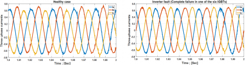
In this study, the output of the photovoltaic array is simulated using a programmable Chroma 62150H-1000S solar panel simulator, which enables the manipulation of environmental conditions (G and T). The electrical grid is represented by a programmable AC source, the Chroma 61511 network simulator. A D Space 1104 digital controller serves as the platform for implementing the control scheme and for data acquisition. The control strategy, such as (VOC), is coupled with (SVPWM) to regulate active and reactive power based on grid-side measurements. Synchronization of the output voltage with the grid voltage is achieved through a Phase-Locked Loop (PLL). The alternating current employed in this research plays a protective role, particularly during the injection of seven real-world defects, as illustrated in Figure 2.
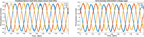
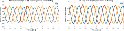
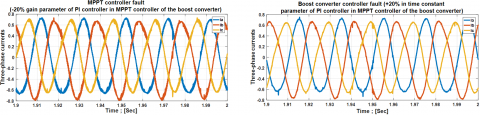
Figure 2. Three-phase currents of a healthy case and seven real faults were injected into a GPV system
This control system employs the (PSO) technique to achieve Maximum Power Point Tracking (MPPT) when the available power is below the nominal level ($P_{Available}$ ≤ $P_{Limit}$). Conversely, it transitions into an Intermediate Power Point Tracking (IPPT) mode when the available power exceeds this threshold ($P_{Available}$ > $P_{Limit}$) [31].
Additional insights and detailed explanations regarding the measurement processes, estimation techniques, and the specific faults analyzed in the system can be found in reference [32].
This grid-connected photovoltaic system offers reliable and precise fault data, which serves as the foundation for our fault identification approach. To achieve this objective, we employed two machine learning techniques: Extreme Learning Machine (ELM) and Support Vector Machine (SVM).
In 2006, Huang proposed a new learning algorithm called ELM (Extreme Learning Machine) for neural networks with a single hidden layer (SLFN) [33]. This algorithm chooses the nodes hidden randomly and estimates the exit weights of the SLFN. The ELM learning speed is considerably faster than that of traditional algorithms in Feedforward neural networks, such as retro propagation algorithm, while having a good generalization capacity. This technique is based on a three -step learning model [34]:
Figure 3. Schema of extreme learning machine (ELM) [35]
The initial structure of the extreme learning machine is illustrated in Figure 3 [35]. We have the ELM's inputs and exits; They are defined as follows:
$X=\left[\begin{array}{lll}x_{11} & \ldots & x_{1 Q} \\ x_{n 1} & \ldots & x_{n Q}\end{array}\right] ; T=\left[\begin{array}{lll}t_{11} & \ldots & t_{1 Q} \\ t_{m 1} & \ldots & t_{m Q}\end{array}\right]$ (4)
where,
The weights connecting the input layer to the hidden layer were initialized randomly.
$W=\left[\begin{array}{lll}w_{11} & \ldots & w_{1 m} \\ w_{m 1} & \ldots & w_{n m}\end{array}\right]$ (5)
Here, '$w_{ij}$' denotes the weights that connect the neurons of the input layer, '$j^{th}$' to the neurons of the hidden layer, 'i'.
The Extreme Learning Machine considers the weights between the hidden layer and the output layer as a matrix noted generally $\beta$, and these can be expressed as follows:
$\beta=\left[\begin{array}{lll}\beta_{11} & \ldots & \beta_{1 m} \\ \beta_{l 1} & \ldots & \beta_{k m}\end{array}\right]$ (6)
Here, '$\beta_{ij}$' signifies the weights that connect the neurons of the hidden layer '$j^{th}$' to the neurons of the output layer '$k^{th}$'.
In an ELM, the biases (or thresholds) of the hidden layer neurons are assigned randomly. This contrasts with traditional neural networks, where both weights and biases are iteratively updated using backpropagation. Instead, ELM generates these biases only once, randomly, and they remain unchanged throughout the entire learning phase.
$B=\left[\begin{array}{llll}b_1 & b_2 & \ldots & b_n\end{array}\right]^{\prime}$ (7)
The Extreme Learning Machine (ELM) selects the network's activation function 'g(x)'. As illustrated in Figure 3, the resulting output matrix 'T' can then be represented by the following equation:
$T=\left[\begin{array}{lll}t_{11} & \ldots & t_{1 Q} \\ t_{m 1} & \ldots & t_{m Q}\end{array}\right]_{m \times Q}$ (8)
Each column vector within the output matrix 'T' is defined by the following expression:
$\begin{array}{r}t_j=\left[\begin{array}{c}t_{1 j} \\ t_{2 j} \\ \cdots \\ t_{m j}\end{array}\right]=\left[\begin{array}{cc}\sum_{i=1}^l \beta_{i 1} g\left(w_j x_j+b_i\right) \\ \sum_{i=1}^l \beta_{i 2} g\left(w_j x_j+b_i\right) \\ \sum_{i=1}^l \beta_{i m} g\left(w_j x_j+b_i\right)\end{array}\right](j=1,2,3, \ldots, Q)\end{array}$ (9)
From Eq. (8) and Eq. (9), we obtain:
$H \beta=T^{\prime}$ (10)
where,
For a unique and minimum-error solution, the values of the weight matrix '$\beta$' are determined using the least squares method [36, 37].
$\beta=H^{\dagger} T^{\prime}$ (11)
where, $H^{\dagger}$ is the generalized opposite of Moore-Penrose of the matrix H.
To enhance the network's generalization ability and stabilize the results, a regularization term is added to $\beta$ [38].
Should the hidden layer have a lower neuron count compared to the training set size, '$\beta$' can be expressed as:
$\beta=\left(\frac{I}{\lambda}+H^{\prime} H\right)^{-1} H^{\prime} T^{\prime}$ (12)
where,
Should the hidden layer have a higher neuron count compared to the learning set size, '$\beta$' can be expressed as follows [40]:
$\beta=H^{\prime}\left(\frac{I}{\lambda}+H H^{\prime}\right)^{-1} T^{\prime}$ (13)
The support vector machine (SVM) is a supervised learning model developed by Vapnik and his team with AT&T Laboratories, mainly intended for binary classification and regression applications. It was successfully used in various fields, including exploration of data mining, bioinformatics, as well as recognition of manuscript characters or digital objects [41, 42].
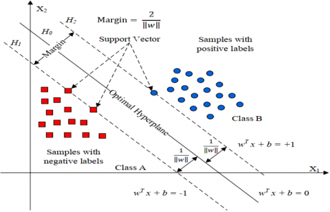
The fundamental idea of a Support Vector Machine (SVM) is to classify data by determining the optimal hyperplane that achieves the widest possible separation between different classes. This optimal separation is defined as the margin, the largest distance between any two support vectors. The data points that lie closest to this separating hyperplane are termed support vectors. Initially conceived for binary classification tasks (involving '$N_C$ = 2' class separation), SVMs can be adapted for multiclass classification (meaning '$N_C$ > 2’ or more classes) through widely used techniques such as one-versus-one or one-versus-all [43].
The fundamental concept of a linear Support Vector Machine (SVM) involves distinguishing between two categories of data points within a two-dimensional feature space, as shown in Figure 4. In this simplified scenario, the optimal hyperplane takes the form of a line. Let 'D' represent a dataset comprising 'n' samples, each residing in a 'd' dimensional space. Each of these samples is assigned to one of two classes:
Learning data is represented in the following form:
$\begin{gathered}D=\left\{\left(x_i, y_i\right), 1 \leq i \leq n, x_i \in R^d, y_i\right. \in\{-1,+1\}\}\end{gathered}$ (14)
As Figure 4 demonstrates with linearly separable data, while various hyperplanes can separate the two classes, the optimal decision rule is obtained by selecting the one that yields the largest margin between them.
Figure 4. Basic idea of SVM [43]
Therefore, the primary goal is to determine the optimal hyperplane '$H_0$' and the two parallel support vector lines '$H_1$ and $H_2$', situated equidistantly from it, while ensuring that no data point falls within the region defined by these two lines [44-46].
The mathematical expressions for the hyperplane and its corresponding support vector lines are given by:
$\left\{\begin{array}{c}H_1: w^T x_i+b=-1 \\ H_0: w^T x_i+b=0 \\ H_2: w^T x_i+b=+1\end{array}\right.$ (16)
The separation between '$H_1$ or $H_2$' and '$H_0$' is mathematically expressed in Eq. (13). Eq. (17), on the other hand, gives the distance between the two support vectors '$H_1$ and $H_2$'.
Distance between $H_{1 \| 2}$ and $H_0=\frac{\left|w^T x_i+\mathrm{b}\right|}{\|w\|}=\frac{1}{\|w\|}$ (16)
Distance between $H_1$ and $H_2=$ Margin $=\frac{2}{\|w\|}$ (17)
As a result, Eq. (17) indicates that to achieve the largest possible margin, it is essential to minimize the standard norm of the vector '$\|w\|=\sqrt{w^T w}$', while adhering to the conditions specified in Eq. (18) which ensure no samples fall within the support vector boundaries.
$\begin{cases}w^T x_i+b \leq-1 & { for } \quad y_i=-1 \\ w^T x_i+b \geq+1 & { for } \quad y_i=+1\end{cases}$ (18)
We can combine these equations to obtain:
$y_i\left(w^T x_i+b\right) \geq 1 \quad \forall i$ (19)
$\left\{\begin{array}{l}\left. { Minimize: } \frac{1}{2} w^T w\right\} { Maximize\, Margin } \\ { Subject\, to: }\, y i\left(w^T x_i+b\right) \geq 1\end{array}\right.$ (20)
The optimization problem expressed in Eq. (20), which is subject to constraints, can be tackled using Lagrange multipliers '$a_i$ ≥ 0', leading to what is termed the dual formulation. This dual problem is equivalent to a quadratic programming problem, solvable with tools like the quadprog solver in the Matlab Optimization ToolboxTM.
$L(w, b, \alpha)=\frac{1}{2} w^T w+\sum_{i=1}^n \alpha_i\left(1-\left(y_i w^T x_i+b\right)\right)$ (21)
$\left\{\begin{array}{c}\frac{\partial L}{\partial w}=0 \Rightarrow w=\sum_{i=1}^n \alpha_i y_i x_i \\ \frac{\partial L}{\partial b}=0 \Rightarrow \sum_{i=1}^n \alpha_i y_i=0\end{array}\right.$ (22)
By substituting Eq. (22) in Eq. (21), we can derive the dual formulation from Eq. (23).
$L_D=\sum_{i=1}^n \alpha_i-\frac{1}{2} \sum_{i=1}^n \sum_{j=1}^n \alpha_i \alpha_j y_i y_j x_i^T x_j$ (23)
In cases where the data points cannot be divided by a linear boundary, a necessary step is to pre-process the data by transforming the input vector 'x' into a characteristic space of higher dimensionality '$\emptyset(x)$'. This method is known as the kernel trick [44].
$L_D=\sum_{i=1}^n \alpha_i-\sum_{i=1}^n \sum_{j=1}^n \alpha_i \alpha_j y_i y_j \underbrace{\varnothing\left(x_i^T\right) \varnothing\left(x_j\right)}_{K\left(x_i, x_j\right)}$ (24)
A variety of kernel functions can be employed, including sigmoid, polynomial, and radial basis function (Gaussian) kernels [47]. In both the SVM modules developed for problem detection and fault diagnosis in this work, the fundamental radial basis function (RBF) kernel is utilized.
$K\left(x_i, x_j\right)=exp \left(-\frac{\|x i-x j\|^2}{2 \sigma^2}\right)$ (25)
This work adopts the One-Versus-One Multiclass SVM approach within its defect detection module to distinguish between seven failure modes in grid-connected photovoltaic systems operating under MPPT. This technique operates by constructing a series of binary classifiers, and the number necessary for this strategy can be determined using the subsequent formula:
$\frac{N_C\left(N_C-1\right)}{2}$ (26)
Feature extraction plays a vital role in data analysis and classification tasks. Key steps in a classification problem include signal preprocessing, extraction of relevant features, feature selection for dimensionality reduction, and classification using a suitable algorithm. Extracting meaningful parameters can significantly enhance the reliability of fault diagnosis. In this study, five statistical features (as shown in Table 1) are derived from the data under various fault conditions. These features serve as input vectors for training and testing the ELM and SVM models to determine whether the system is operating under normal conditions or exhibiting faults [48].
Table 1. Statistical features [48]
|
Statistical Features |
Equation |
|
Minimum |
Min(x) |
|
Maximum |
Max(x) |
|
Kurtosis |
$\begin{gathered}\frac{1}{N} \sum_{i=0}^N \bar{x}_i^4-\frac{3}{N^2}\left(\sum_{i=0}^N x_i^2\right)^2-\frac{4}{N} \bar{x}\left(\sum_{i=0}^N x_i^2\right)+\frac{12}{N} \bar{x}^2\left(\sum_{i=0}^N x_i^2\right)-6 \bar{x}^4\end{gathered}$ |
|
Mean |
$\frac{1}{N} \sum_{i=0}^N x_i$ |
|
Skewness |
$\frac{1}{N} \sum_{i=0}^N x_i^3-\frac{3}{N} \bar{x}\left(\sum_{i=0}^N x_i^2\right)+2 \bar{x}^3$ |
where,
To achieve a more efficient seven-fault classification, the BGWO and BDE feature selection algorithms are implemented to reduce the dimensionality of the feature space.
Feature selection is a critical stage in pattern recognition. In this study, our focus is on employing optimization algorithms to perform this selection process.
6.1 Binary grey wolf optimization (BGWO)
The Binary Grey Wolf Optimization (BGWO) method is recommended and employed in this research to identify the most suitable subset of characteristics for the classification tasks. The Gray Wolf Optimization (GWO) algorithm, on which the BGWO is based, is inspired by the gray wolves' hunting behavior. This behavior is structured according to a social hierarchy comprising:
The main use of optimization by the binary gray wolf (BGWO) is the selection of characteristics (feature selection) [49]. This method is particularly effective in reducing the dimensionality of data while retaining the most relevant information, which improves the accuracy of classification models and reduces their computational complexity. By representing each solution as a binary vector (where each bit indicates whether a characteristic is selected or not), the BGWO explores the search space to find the optimal subset of explanatory variables.
Algorithm 1 illustrates the stages of optimization by the Gray Binary Group (binary optimization of the gray wolf, BGWO) [50].
|
Algorithm 1: BGWO algorithm |
|
|
1: |
Define population size N, and maximum number of generation $G_{max}$. |
|
2: |
Generate an initial random uniformly distributed population of N vectors. |
|
3: |
Find the objective function values for all members of the population. |
|
4: |
While G < $G_{max}$ do |
|
5: |
for n = 1 to N do |
|
6: |
Update the $n_{t h}$ vector using: |
|
7: |
$\begin{gathered}W_{G+1,\,i}=\left\{\begin{array}{l}1, \quad \text { if } S\left(\frac{W_{1, i}+W_{2, i}+W_{3, i}}{3}\right) \geq \operatorname{rand}() . \\ 0,\quad {otherwise.}\end{array}\right.\end{gathered}$ |
|
8: |
End for |
|
9: |
Update u, $C_1$, and $C_2$ |
|
10: |
Update $W_a$, $W_\beta$, and $W_\delta$ |
|
11: |
Set: G = G + 1 |
|
12: |
End while |
6.2 Binary differential evolution (BDE)
When tackling classification tasks with numerous features, selecting a subset of the most informative ones is crucial. This process streamlines the classifier's computations by eliminating unnecessary data points and can potentially enhance its ability to correctly categorize instances by focusing on the most pertinent attributes. A key difficulty in multi-class classification lies in identifying a smaller group of features that can maintain a comparable level of accuracy to when the entire original set is used.
The following paragraphs explain the working principles of differential evolution and the method applied to optimize the extreme learning machine (ELM). Moreover, the basic theory, relevant definitions, and the mathematical expressions for the operators of binary differential evolution (BDE) are presented, alongside other functionalities of this approach. In this study, binary differential evolution is employed, and its fundamental theoretical basis is the same as that of conventional differential evolution. The main differences between them are in the way their operators are structured.
Introduced by the study [51], differential evolution (DE) is a widely recognized optimization algorithm, cited by the study [52] as being among the most popular. As a population-based optimizer, it's designed to tackle a range of optimization challenges by evaluating an objective function (OF). The method starts with a randomly generated set of initial solutions, which are subsequently combined to produce a refined group of individuals.
According to the study [53], an algorithm of differential evolution (DE) must have four fundamental capacities:
1). An effective exploration of the research space,
2). an appropriate exploitation of promising solutions,
3). The prevention of stagnation in iterations,
4). Prevention of premature convergence to sub-optimal solutions.
The field of differential evolution (DE) has seen many advancements and combinations with other algorithms over time [54-57]. For a comprehensive understanding of the latest and most sophisticated research in differential evolution, reference [52] is recommended.
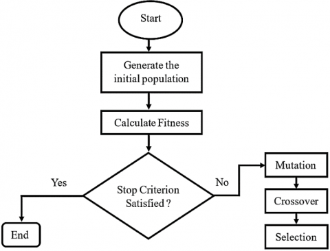
Differential evolution is characterized by its straightforward design, making it relatively easy to grasp. In essence, it employs genetic operators, namely mutation, crossover, and selection on a population 'G' in generation '$X^{(G)}$' to produce a subsequent population in generation '$X^{(G+1)}$'. Figure 5 provides a visual representation of this optimization process through a flowchart.
Figure 5. Flowchart of the stages of differential evolution [52]
Binary differential evolution (BDE) operates based on the same fundamental principles as differential evolution (DE) and proceeds through four distinct phases.
The equations presented in this section will henceforth pertain to binary differential evolution (BDE).
In binary differential evolution (BDE), the process starts with the generation of a random population '$X^{(0)}$', which includes '$N_{ind}$' individuals, each having '$N_{gen}$' genes, according to Eq. (27).
$x_{n_{ {ind }}, n_{ {gen }}}^{(0)}=\left\{\begin{array}{lc}1, & { if \,\,rand } \geq 0.5 \\ 0 & { otherwise }\end{array}\right.$ (27)
Here, '$n_{ {ind }}=1,2, \ldots, N_{{ind }}$' represents the individuals, '$n_{ {gen}}=1,2, \ldots, N_{{gen}}$' the genes, and '0' denotes the initial population. (Rand) signifies a random number within the range '[0, 1]'. It's important to note that each individual '$x_{n_{ {ind }}}^{(G)}$' in any generation 'G' is also referred to as a Target Vector. Following the initialization, the fitness of each individual within the population is evaluated using a chosen objective function. Subsequently, a mutation operator is applied to introduce variation or change within the population. One example of a mutation process, among many possibilities, is provided by Eq. (28).
$v_{n_{ {ind }}, n_{ {gen }}^{(G+1)}}=\left\{\begin{array}{cc}1, & { if\, rand } \geq P\left(x_{n_{ {ind }}, n_{ {gen }}}^{(G)}\right) \\ 0 & { otherwise }\end{array}\right.$ (28)
where, '$v_{n_{{ind }}, n_{{gen }}}^{(G+1)}$' represents the mutant vector obtained, and '$P\left(x_{n_{ {ind }}, n_{{gen }}}^{(G)}\right)$' designates the probability value, which can be determined, for example, using the probability estimate operator (PEO) [58]. Once the mutation has been made, the crossing operator can be applied to improve the diversity of the population and generate a test vector '$u_{n_{{ind }}, n_{{gen }}}^{(G+1)}$'.
Through a random combination process, this operator merges the target vector and the mutant vector, as described by Eq. (29).
$\begin{aligned} & u_{n_{ {ind }}, n_{ {gen }}}^{(G+1)}=\left\{\begin{array}{lr}v_{n_{ {ind }}, n_{ {gen }}}^{(G+1)}, & { if \,\,rand } \geq { CR \,or \,} n_{ {gen }}= { I \,rand } \\ x_{n_{ {ind }}^{(G)}, n_{ {gen }}}^{(G)}, & { otherwise }\end{array}\right.\end{aligned}$ (29)
In this equation, 'CR' stands for the crossover rate, a value chosen within the bounds of 0 and 1. The symbol 'I rand' represents a randomly selected gene index from the set of all gene positions, '1, 2, ..., $N_{gen}$'. Finally, 'G' and 'G + 1' are used to denote the current and the succeeding generations.
Following the mutation and crossover operations, the subsequent step involves applying the selection operator, which is based on the fitness values of both the target and trial vectors. This selection process is governed by Eq. (30).
$x_{n_{{ind }}^{(G+1)}}^{(G)}=\left\{\begin{array}{lc}u_{n_{ {ind }}}^{(G+1)}, & { if\, } f i t_{u_{n_{{ind }}^{(G+1)}}} \geq f i t_{x_{n_{ {ind }}^{(G)}}} \\ x_{n_{{ind }}}^{(G)}, & { otherwise }\end{array}\right.$ (30)
Following the application of the operators, a new population '$X^{(G+1)}$' for the next generation, '$x_1^{(G+1)}, x_2^{(G+1)}, \ldots, x_{N_{ {ind }}}^{(G+1)}$', is formed. This cycle of applying the operators is repeated iteratively until a termination condition is satisfied, for instance, when the maximum number of generations is reached.
For additional information on the Differential Evolution (DE) algorithm, we can refer to the study [51], which is the first author. An in-depth study of the fundamental concepts, variants, and applications of algorithms [59]. The theoretical study of DE, including the analysis of convergence, differential change, crossroads, and the diversity of the population [60]. Finally, specific information on the binary version of the algorithm, Binary Differential Evolution (BDE) [61, 62].
This study considers the seven fault scenarios and one healthy operating condition in grid-connected photovoltaic (PV) systems under Maximum Power Point Tracking (MPPT) mode, as detailed in Table 2 (labeled F0M to F7M).
Table 2. Faults injected in the GPV system [31]
|
Default |
Type |
Description |
|
F0M |
Healthy case |
Healthy case |
|
F1M |
Inverter fault |
Complete failure in one of the six IGBTs |
|
F2M |
Feedback Sensor fault |
One phase sensor fault 20% |
|
F3M |
Grid anomaly |
Intermittent voltage sags |
|
F4M |
PV array mismatch |
10 to 20% nonhomogeneous partial shading |
|
F5M |
PV array mismatch |
15% open circuit in PV array |
|
F6M |
MPPT controller fault |
-20% gain parameter of PI controller in MPPT controller of the boost converter |
|
F7M |
Boost converter controller fault |
+20% in time constant parameter of PI controller in MPPT controller of the boost converter |
We used the flowchart in Figure 6 to achieve our objective to detect these seven defects by using 70% of the dataset to train ELM and SVM classifiers and the remainder for testing.
Figure 6. Flowchart of the suggested architecture
The application of the learning machines (ELM and SVM) with BGWO and BDE and their tuning parameters that give us the best results are shown in Table 3.
Table 3. The best results of ELM and SVM with (BGWO and BDE)
|
Accuracy |
Tuning Parameters For |
|||
|
BGWO |
BDE |
|||
|
Parameter |
Values |
Parameter |
Values |
|
|
Population (N) |
10 |
Population |
10 |
|
|
Maximum number of iterations |
100 |
Maximum number of iterations |
100 |
|
|
Search domain |
[0 1] |
Crossover rate (CR) |
0.9 |
|
|
ELM |
SVM |
ELM |
SVM |
|
|
Best Training Accuracy |
100% with 278 Neurons |
100% |
100% with 77 Neurons |
98.92% |
|
Best Testing Accuracy |
99.16% with 62 Neurons |
96.66% |
98.33% with 172 Neurons |
95% |
To enhance the efficiency of the seven-fault classification by reducing the number of features, binary grey wolf optimization (BGWO) and binary differential evolution (BDE) were applied for feature selection. According to the results in Table 4, the Extreme Learning Machine (ELM) utilizing BGWO for feature selection outperformed other techniques, reaching a high accuracy of 99.16% in detecting faults.
Table 4. The accuracy of each classifier
|
Classifiers and Time |
Features Selections |
|||||||
|
Without Optimization |
BGWO |
BDE |
||||||
|
Training (%) |
Testing (%) |
Training (%) |
Testing (%) |
Training (%) |
Testing (%) |
|||
|
ELM |
100 |
95 |
100 |
99.16 |
100 |
98.33 |
||
|
Time; [Sec] |
31.361 |
20.0297 |
43.9597 |
19.2206 |
42.3499 |
20.9613 |
||
|
SVM |
Kernel functions |
RBF |
100 |
85.83 |
100 |
96.66 |
98.92 |
95 |
|
Time ; [Sec] |
5.5486 |
0.043865 |
3.1925 |
0.041497 |
3.36 |
0.037256 |
||
|
Linear |
95 |
91.6667 |
78.5714 |
72.5 |
85.3571 |
79.1667 |
||
|
Time ; [Sec] |
3.322 |
0.029982 |
3.3127 |
0.025633 |
3.1283 |
0.028743 |
||
|
Polynomial |
100 |
97.5 |
88.5714 |
85.8333 |
100 |
94.1667 |
||
|
Time ; [Sec] |
3.2901 |
0.032833 |
3.1712 |
0.032326 |
3.1946 |
0.032258 |
||
8.1 Classification Using Support Vector Machine (SVM)
This section presents the classification results of the Support Vector Machine (SVM) optimized using two binary metaheuristic algorithms: Binary Differential Evolution (BDE) and Binary Grey Wolf Optimization (BGWO).
8.1.1 Classification using SVM with BDE optimization algorithm
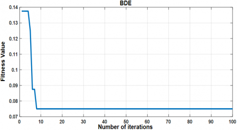
To improve the classification accuracy, the Binary Differential Evolution (BDE) algorithm was employed for feature selection before training the SVM classifier. The convergence behavior of the BDE algorithm during optimization is shown in Figure 7, which illustrates a gradual decrease in the cost function over successive iterations.
Figure 7. Convergence of the cost function optimized by the binary differential evolution (BDE) algorithm
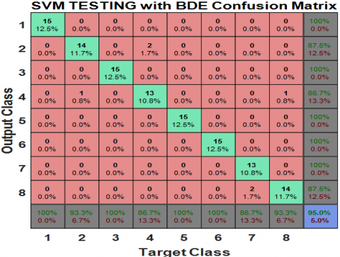
The performance of the SVM classifier optimized with BDE is depicted in the confusion matrix in Figure 8. As can be seen, the model achieves a respectable classification performance, although some misclassifications still occur. The final cost function value attained by the BDE algorithm in the case of SVM $C_{fBED} = 0.075$.
Figure 8. Confusion matrix of SVM based on binary differential evolution (BDE) algorithm
8.1.2 Classification using SVM with BGWO optimization algorithm
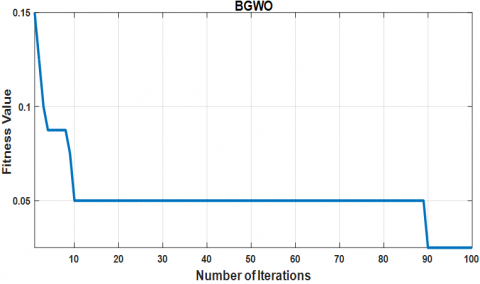
Similarly, Binary Grey Wolf Optimization (BGWO) was used to optimize feature selection for the SVM classifier. As shown in Figure 9, the BGWO algorithm demonstrates a faster convergence rate compared to BDE, reaching a lower cost function value more rapidly. The final cost function value for BGWO in this case is $C_{fBGWO} = 0.025$, indicating superior performance over BDE.
Figure 9. Convergence of the cost function optimized by the binary grey wolf optimization (BGWO) algorithm
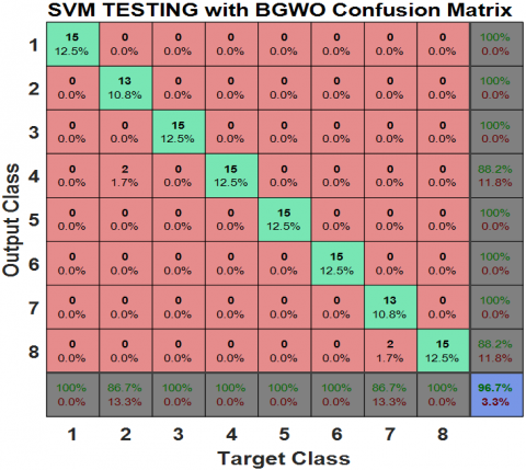
The corresponding confusion matrix for the BGWO-optimized SVM is presented in Figure 10. The results clearly demonstrate improved classification accuracy, with fewer misclassified samples than the BDE-based approach. Overall, BGWO proves to be more effective in enhancing SVM performance.
Figure 10. Confusion matrix of SVM based on binary grey wolf optimization (BGWO) algorithm
8.2 Classification using extreme learning machine (ELM)
Extreme Learning Machine (ELM) classifiers were also evaluated using both BDE and BGWO optimization techniques for feature selection. The ELM's performance is sensitive to three parameters: input weights, bias values, and the number of hidden layer neurons. In this study, input weights and biases were randomly initialized, and the output weights were computed using the closed-form solution described in Eqs. (12) and (13), with a sigmoid activation function applied.
8.2.1 Classification using ELM with BDE optimization algorithm
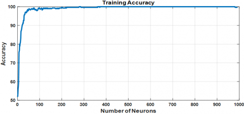
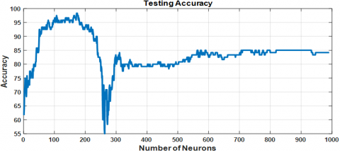
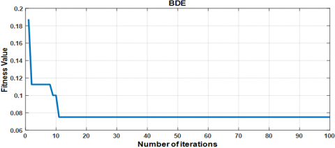
Figures 11(a) and 11(b) show the training and testing accuracy of the ELM classifier when optimized with the BDE algorithm. The model reaches a relatively high testing accuracy with a specific number of hidden neurons. The convergence of the cost function during optimization is shown in Figure 12, which reflects the algorithm’s progression towards an optimal solution. The final cost function value for the BDE-optimized ELM is $C_{fBDE} = 0.075$.
(a)Training accuracy
(b) Testing accuracy
Figure 11. Accuracy of ELM with BDE optimization algorithm
Figure 12. Convergence of the cost function optimized by the binary differential evolution (BDE) algorithm
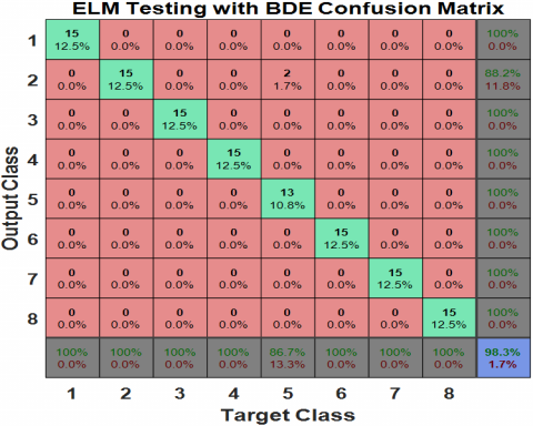
The classification results are further detailed in the confusion matrix shown in Figure 13, where the model misclassifies one sample, resulting in an error rate of 10.8%.
Figure 13. Confusion matrix of ELM based on binary differential evolution (BDE) algorithm
8.2.2 Classification using ELM with BGWO optimization algorithm
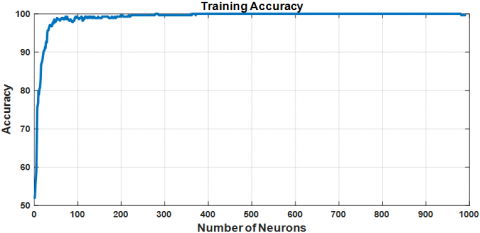
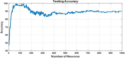
Training and testing accuracies for the ELM using BGWO-optimized feature selection are illustrated in Figures 14(a) and 14(b), respectively. This approach yields superior testing accuracy, reaching 99.16% with 62 hidden layer neurons, the optimal architecture found in this study.
(a) Training accuracy
(b) Testing accuracy
Figure 14. Accuracy of ELM using feature selection based on BGWO
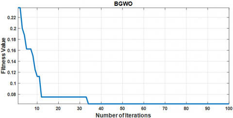
The convergence behavior of the BGWO algorithm for ELM is shown in Figure 15, which confirms the faster convergence and better final cost value $C_{fBGWO} = 0.0625$, compared to BDE.
Figure 15. Convergence of the cost function optimized by the binary grey wolf optimization (BGWO) algorithm
The final confusion matrix is displayed in Figure 16, where only one sample is misclassified, corresponding to an error rate of 11.7%. While this is marginally higher than the error rate observed with BDE, the significantly higher testing accuracy indicates that BGWO provides better generalization for the ELM model.
Figure 16. Confusion matrix of ELM based on binary grey wolf optimization (BGWO) algorithm
Early detection and diagnosis make it possible to limit damage and maintain the other components of the photovoltaic system connected to the network by studying the influence of defects and their behavior in the event of dysfunction. This work offers a new contribution for the detection of seven defects extracted from a real database, which can affect a photovoltaic system connected to the network operating in MPPT mode. The proposed diagnostic method is based on artificial intelligence, represented by Extreme Learning Machine (ELM) models and Support Vector Machine (SVM), assisted by BGWO and BDE optimization algorithms. The results obtained clearly show that the ELM approach, associated with the BGWO optimization algorithm based on statistical parameters, offers high precision (99.16%). This highlights its importance in identifying the various defects in PV systems connected to the network in MPPT mode, while reducing the severity of the breakdowns. In addition, based on these results, future work could apply the ELM assisted by other optimization algorithms such as the principal component analysis (PCA) or the Binary Harris Hawk Optimization (BHHO) algorithm in other areas of diagnostics, such as electric machines or any technological process.
The authors extend their heartfelt gratitude to the Signals and Systems Laboratory group at the Institute of Electrical and Electronics Engineering, University M’Hamed Bougara of Boumerdes, Algeria, for supplying the database of fault scenarios in grid-connected photovoltaic systems operating under MPPT mode, utilized in this paper. Accessibility of data the database utilized in this paper was acquired in January 2025 from the data accessible at [http://doi.org/10.17632/n76t439f65.1].
[1] Rynska, E. (2022). Review of pv solar energy development 2011–2021 in central european countries. Energies, 15(21): 8307. https://doi.org/10.3390/en15218307
[2] Chikunov, S.O., Gutsunuk, O.N., Ivleva, M.I., Elyakova, I.D., Nikolaeva, I.V., Maramygin, M.S. (2018). Improving the economic performance of Russia's energy system based on the development of alternative energy sources. International Journal of Energy Economics and Policy, 8(6): 382-391. https://doi.org/10.32479/ijeep.7025
[3] Gunduz, H., Jayaweera, D. (2018). Reliability assessment of a power system with cyber-physical interactive operation of photovoltaic systems. International Journal of Electrical Power & Energy Systems, 101: 371-384. https://doi.org/10.1016/j.ijepes.2018.04.001
[4] International Electrotechnical Commission. (2016). IEC Photovoltaic (PV) arrays–Design requirements. International Electrotechnical Commission: Geneva, Switzerland.
[5] De la Parra, I., Muñoz, M., Lorenzo, E., García, M., Marcos, J., Martínez-Moreno, F. (2017). PV performance modelling: A review in the light of quality assurance for large PV plants. Renewable and Sustainable Energy Reviews, 78: 780-797. https://doi.org/10.1016/j.rser.2017.04.080
[6] Kumar, N.M., Dasari, S., Reddy, J.B. (2018). Availability factor of a PV power plant: Evaluation based on generation and inverter running periods. Energy Procedia, 147: 71-77. https://doi.org/10.1016/j.egypro.2018.07.035
[7] Cai, B., Liu, Y., Ma, Y., Huang, L., Liu, Z. (2015). A framework for the reliability evaluation of grid-connected photovoltaic systems in the presence of intermittent faults. Energy, 93: 1308-1320. https://doi.org/10.1016/j.energy.2015.10.068
[8] Madeti, S.R., Singh, S.N. (2017). Online fault detection and the economic analysis of grid-connected photovoltaic systems. Energy, 134: 121-135. https://doi.org/10.1016/j.energy.2017.06.005
[9] Saha, S., Haque, M.E., Tan, C.P., Mahmud, M.A., Arif, M.T., Lyden, S., Mendis, N. (2020). Diagnosis and mitigation of voltage and current sensors malfunctioning in a grid connected PV system. International Journal of Electrical Power & Energy Systems, 115: 105381. https://doi.org/10.1016/j.ijepes.2019.105381
[10] Naik, J., Dhar, S., Dash, P.K. (2019). Adaptive differential relay coordination for PV DC microgrid using a new kernel based time-frequency transform. International Journal of Electrical Power & Energy Systems, 106: 56-67. https://doi.org/10.1016/j.ijepes.2018.09.043
[11] Huka, G.B., Li, W., Chao, P., Peng, S. (2018). A comprehensive LVRT strategy of two-stage photovoltaic systems under balanced and unbalanced faults. International Journal of Electrical Power & Energy Systems, 103: 288-301. https://doi.org/10.1016/j.ijepes.2018.06.014
[12] Pillai, D.S., Rajasekar, N. (2018). Metaheuristic algorithms for PV parameter identification: A comprehensive review with an application to threshold setting for fault detection in PV systems. Renewable and Sustainable Energy Reviews, 82: 3503-3525. https://doi.org/10.1016/j.rser.2017.10.107
[13] Bhagavathy, S., Pearsall, N., Putrus, G., Walker, S. (2019). Performance of UK distribution networks with single-phase PV systems under fault. International Journal of Electrical Power & Energy Systems, 113: 713-725. https://doi.org/10.1016/j.ijepes.2019.05.077
[14] Dashti, R., Ghasemi, M., Daisy, M. (2018). Fault location in power distribution network with presence of distributed generation resources using impedance based method and applying π line model. Energy, 159: 344-360. https://doi.org/10.1016/j.energy.2018.06.111
[15] Hong, Y.Y., Pula, R.A. (2022). Methods of photovoltaic fault detection and classification: A review. Energy Reports, 8: 5898-5929. https://doi.org/10.1016/j.egyr.2022.04.043
[16] El-Rashidy, M.A. (2022). An efficient and portable solar cell defect detection system. Neural Computing and Applications, 34(21): 18497-18509. https://doi.org/10.1007/s00521-022-07464-2
[17] Manohar, M., Koley, E., Ghosh, S., Mohanta, D.K., Bansal, R.C. (2020). Spatio-temporal information based protection scheme for PV integrated microgrid under solar irradiance intermittency using deep convolutional neural network. International Journal of Electrical Power & Energy Systems, 116: 105576. https://doi.org/10.1016/j.ijepes.2019.105576
[18] El-Banby, G.M., Moawad, N.M., Abouzalm, B.A., Abouzaid, W.F., Ramadan, E.A. (2023). Photovoltaic system fault detection techniques: A review. Neural Computing and Applications, 35(35): 24829-24842. https://doi.org/10.1007/s00521-023-09041-7
[19] Kurukuru, V.S.B., Blaabjerg, F., Khan, M.A., Haque, A. (2020). A novel fault classification approach for photovoltaic systems. Energies, 13(2): 308. https://doi.org/10.3390/en13020308
[20] Voulodimos, A., Doulamis, N., Doulamis, A., Protopapadakis, E. (2018). Deep learning for computer vision: A brief review. Computational Intelligence and Neuroscience, 2018(1): 7068349. https://doi.org/10.1155/2018/7068349
[21] Pillai, D.S., Rajasekar, N. (2018). A comprehensive review on protection challenges and fault diagnosis in PV systems. Renewable and Sustainable Energy Reviews, 91: 18-40. https://doi.org/10.1016/j.rser.2018.03.082
[22] Lu, S., Phung, B.T., Zhang, D. (2018). A comprehensive review on DC arc faults and their diagnosis methods in photovoltaic systems. Renewable and Sustainable Energy Reviews, 89: 88-98. https://doi.org/10.1016/j.rser.2018.03.010
[23] Brooks, B. (2011). The bakersfield fire: A lesson in ground-fault protection. SolarPro Mag, 62: 62-70.
[24] Memon, A.A., Kauhaniemi, K. (2015). A critical review of AC Microgrid protection issues and available solutions. Electric Power Systems Research, 129: 23-31. https://doi.org/10.1016/j.epsr.2015.07.006
[25] Cui, M., Wang, J., Chen, B. (2020). Flexible machine learning-based cyberattack detection using spatiotemporal patterns for distribution systems. IEEE Transactions on Smart Grid, 11(2): 1805-1808. https://doi.org/10.1109/TSG.2020.2965797
[26] Yang, B., Yu, T., Zhang, X., Li, H., Shu, H., Sang, Y., Jiang, L. (2019). Dynamic leader based collective intelligence for maximum power point tracking of PV systems affected by partial shading condition. Energy Conversion and Management, 179: 286-303. https://doi.org/10.1016/j.enconman.2018.10.074
[27] Yang, B., Zhong, L., Zhang, X., Shu, H., Yu, T., Li, H., Jiang, L., Sun, L. (2019). Novel bio-inspired memetic salp swarm algorithm and application to MPPT for PV systems considering partial shading condition. Journal of Cleaner Production, 215: 1203-1222. https://doi.org/10.1016/j.jclepro.2019.01.150
[28] Mohapatra, A., Nayak, B., Das, P., Mohanty, K.B. (2017). A review on MPPT techniques of PV system under partial shading condition. Renewable and Sustainable Energy Reviews, 80: 854-867. https://doi.org/10.1016/j.rser.2017.05.083
[29] Bakdi, A., Guichi, A., Mekhilef, S., Bounoua, W. (2020). GPVS-faults: Experimental data for fault scenarios in grid-connected PV systems under MPPT and IPPT modes. Mendeley Data, 1: 78. https://doi.org/10.17632/n76t439f65.1
[30] Guichi, A., Berkouk, E.M., Mekhilef, S., Gassab, S. (2018). A new method for intermediate power point tracking for PV generator under partially shaded conditions in hybrid system. Solar Energy, 170: 974-987. https://doi.org/10.1016/j.solener.2018.06.027
[31] Bakdi, A., Bounoua, W., Guichi, A., Mekhilef, S. (2021). Real-time fault detection in PV systems under MPPT using PMU and high-frequency multi-sensor data through online PCA-KDE-based multivariate KL divergence. International Journal of Electrical Power & Energy Systems, 125: 106457. https://doi.org/10.1016/j.ijepes.2020.106457
[32] Guichi, A., Talha, A.B.D.E.L.A.Z.I.Z., Berkouk, E.M., Mekhilef, S., Gassab, S. (2018). A new method for intermediate power point tracking for PV generator under partially shaded conditions in hybrid system. Solar Energy, 170: 974-987. https://doi.org/10.1016/j.solener.2018.06.027
[33] Gao, K., Deng, X., Cao, Y. (2019). Industrial process fault classification based on weighted stacked extreme learning machine. In 2019 CAA Symposium on Fault Detection, Supervision and Safety for Technical Processes (SAFEPROCESS), Xiamen, China, IEEE, pp. 328-332. https://doi.org/10.1109/SAFEPROCESS45799.2019.9213317
[34] Li, L., Zeng, J., Jiao, L., Liang, P., Liu, F., Yang, S. (2019). Online active extreme learning machine with discrepancy sampling for PolSAR classification. IEEE Transactions on Geoscience and Remote Sensing, 58(3): 2027-2041. https://doi.org/10.1109/TGRS.2019.2952236
[35] Souaidia, C., Thelaidjia, T., Chenikher, S. (2023). Independent vector analysis based on binary grey wolf feature selection and extreme learning machine for bearing fault diagnosis. The Journal of Supercomputing, 79(6): 7014-7036. https://doi.org/10.1007/s11227-022-04931-4
[36] Wang, S.J., Chen, H.L., Yan, W.J., Chen, Y.H., Fu, X. (2014). Face recognition and micro-expression recognition based on discriminant tensor subspace analysis plus extreme learning machine. Neural Processing Letters, 39: 25-43. https://doi.org/10.1007/s11063-013-9288-7
[37] Huang, G.B. (2014). An insight into extreme learning machines: Random neurons, random features and kernels. Cognitive Computation, 6: 376-390. https://doi.org/10.1007/s12559-014-9255-2
[38] Wei, J., Liu, H., Yan, G., Sun, F. (2017). Robotic grasping recognition using multi-modal deep extreme learning machine. Multidimensional Systems and Signal Processing, 28: 817-833. https://doi.org/10.1007/s11045-016-0389-0
[39] Fan, Q., Liu, T. (2020). Smoothing l0 regularization for extreme learning machine. Mathematical Problems in Engineering, 2020(1): 9175106. https://doi.org/10.1155/2020/9175106
[40] Xiao, D., Li, B., Mao, Y. (2017). A multiple hidden layers extreme learning machine method and its application. Mathematical Problems in Engineering, 2017(1): 4670187. https://doi.org/10.1155/2017/4670187
[41] Oujaoura, M., Minaoui, B., Fakir, M., El Ayachi, R., Bencharef, O. (2014). Recognition of isolated printed tifinagh characters. International Journal of Computer Applications, 85(1).
[42] Kim, H.C., Pang, S., Je, H.M., Kim, D., Bang, S.Y. (2003). Constructing support vector machine ensemble. Pattern Recognition, 36(12): 2757-2767. https://doi.org/10.1016/S0031-3203(03)00175-4
[43] Badr, M.M., Hamad, M.S., Abdel-Khalik, A.S., Hamdy, R.A. (2019). Fault detection and diagnosis for photovoltaic array under grid connected using support vector machine. In 2019 IEEE Conference on Power Electronics and Renewable Energy (CPERE), Aswan, Egypt, pp. 546-553. https://doi.org/10.1109/CPERE45374.2019.8980103
[44] Yin, Z., Hou, J. (2016). Recent advances on SVM based fault diagnosis and process monitoring in complicated industrial processes. Neurocomputing, 174: 643-650. https://doi.org/10.1016/j.neucom.2015.09.081
[45] Sawitri, D.R., Purnama, I.K.E., Ashari, M. (2012). Detection of electrical faults in induction motor fed by inverter using support vector machine and receiver operating characteristic. Journal of Theoretical and Applied Information Technology, 40(1): 14-21.
[46] Martínez, J., Iglesias, C., Matías, J.M., Taboada, J., Araújo, M. (2014). Solving the slate tile classification problem using a DAGSVM multiclassification algorithm based on SVM binary classifiers with a one-versus-all approach. Applied Mathematics and Computation, 230: 464-472. https://doi.org/10.1016/j.amc.2013.12.087
[47] Kijsirikul, B., Ussivakul, N. (2002). Multiclass support vector machines using adaptive directed acyclic graph. In Proceedings of The 2002 International Joint Conference on Neural Networks. IJCNN'02 (cat. no. 02ch37290), Honolulu, HI, USA, IEEE, 1: 980-985. https://doi.org/10.1109/IJCNN.2002.1005608
[48] Fares, N., Aoulmi, Z., Thelaidjia, T., Ounnas, D. (2022). Learning machine based on optimized dimensionality reduction algorithm for fault diagnosis of rotor broken bars in Induction Machine. European Journal of Electrical Engineering, 24(4): 171. https://doi.org/10.18280/ejee.240402
[49] Emary, E., Zawbaa, H.M., Hassanien, A.E. (2016). Binary grey wolf optimization approaches for feature selection. Neurocomputing, 172: 371-381. https://doi.org/10.1016/j.neucom.2015.06.083
[50] Goudos, S.K., Boursianis, A., Salucci, M., Rocca, P. (2020). Dualband patch antenna design using binary grey wolf optimizer. In 2020 IEEE International Symposium on Antennas and Propagation and North American Radio Science Meeting, Montreal, QC, Canada, pp. 1777-1778. https://doi.org/10.1109/IEEECONF35879.2020.9330100
[51] Storn, R., Price, K. (1997). Differential evolution–a simple and efficient heuristic for global optimization over continuous spaces. Journal of Global Optimization, 11: 341-359. https://doi.org/10.1023/A:1008202821328
[52] Ahmad, M.F., Isa, N.A.M., Lim, W.H., Ang, K.M. (2022). Differential evolution: A recent review based on state-of-the-art works. Alexandria Engineering Journal, 61(5): 3831-3872. https://doi.org/10.1016/j.aej.2021.09.013
[53] Zeng, Z., Zhang, M., Hong, Z., Zhang, H., Zhu, H. (2022). Enhancing differential evolution with a target vector replacement strategy. Computer Standards & Interfaces, 82: 103631. https://doi.org/10.1016/j.csi.2022.103631
[54] Houssein, E.H., Rezk, H., Fathy, A., Mahdy, M.A., Nassef, A.M. (2022). A modified adaptive guided differential evolution algorithm applied to engineering applications. Engineering Applications of Artificial Intelligence, 113: 104920. https://doi.org/10.1016/j.engappai.2022.104920
[55] Pan, J.S., Liu, N., Chu, S.C. (2022). A competitive mechanism based multi-objective differential evolution algorithm and its application in feature selection. Knowledge-Based Systems, 245: 108582. https://doi.org/10.1016/j.knosys.2022.108582
[56] Yi, W., Chen, Y., Pei, Z., Lu, J. (2022). Adaptive differential evolution with ensembling operators for continuous optimization problems. Swarm and Evolutionary Computation, 69: 100994. https://doi.org/10.1016/j.swevo.2021.100994
[57] Luo, N., Lin, W., Jin, G., Jiang, C., Chen, J. (2020). Decomposition-based multiobjective evolutionary algorithm with genetically hybrid differential evolution strategy. IEEE Access, 9: 2428-2442. https://doi.org/10.1109/ACCESS.2020.3047699
[58] Dhaliwal, J.S., Dhillon, J.S. (2021). A synergy of binary differential evolution and binary local search optimizer to solve multi-objective profit based unit commitment problem. Applied Soft Computing, 107: 107387. https://doi.org/10.1016/j.asoc.2021.107387
[59] Das, S., Suganthan, P.N. (2010). Differential evolution: A survey of the state-of-the-art. IEEE Transactions on Evolutionary Computation, 15(1): 4-31. https://doi.org/10.1109/TEVC.2010.2059031
[60] Opara, K.R., Arabas, J. (2019). Differential evolution: A survey of theoretical analyses. Swarm and Evolutionary Computation, 44: 546-558. https://doi.org/10.1016/j.swevo.2018.06.010
[61] GGong, T., Tuson, A.L. (2007). Differential evolution for binary encoding. In Soft Computing in Industrial Applications: Recent and Emerging Methods and Techniques, pp. 251-262. https://doi.org/10.1007/978-3-540-70706-6_24
[62] Doerr, B., Zheng, W. (2020). Working principles of binary differential evolution. Theoretical Computer Science, 801: 110-142. https://doi.org/10.1016/j.tcs.2019.08.025