Khamiss Cheikh*![]() | EL Mostapha Boudi | Rabi Rabi
| EL Mostapha Boudi | Rabi Rabi![]() | Hamza Mokhliss
| Hamza Mokhliss![]()
© 2024 The authors. This article is published by IIETA and is licensed under the CC BY 4.0 license (http://creativecommons.org/licenses/by/4.0/).
OPEN ACCESS
Global competition has driven extraordinary changes in the way firms operate, significantly impacting maintenance functions and emphasizing their critical role in corporate success. To remain competitive, organizations must continuously enhance their maintenance strategies, leading to considerable efforts to improve the economic performance of maintenance for stochastically degrading production systems. This study aims to contribute to robust decision-making in the maintenance of systems vulnerable to gradual deterioration. Our primary objective is to develop criteria that enable the combined assessment of mean economic performance and robustness across various maintenance techniques. The benefit of the suggested criteria is its adaptability to different maintenance strategies, providing a simple yet relevant assessment model. Specifically, this study compares three maintenance strategies: block replacement (BR), periodic inspection and replacement (PIR), and quantile-based inspection and replacement (QIR). These strategies are analyzed using the long-term expected maintenance cost rate as a measure of performance and the variance of maintenance cost per renewal cycle as a measure of robustness. Mathematical cost models are formulated based on the homogeneous Gamma degradation process and probability theory. Using the Monte Carlo method in MATLAB, the study compares these maintenance techniques, applying the proposed criteria to quantify performance and robustness. The study concludes that the developed criteria offer a comprehensive and adaptable framework for evaluating and enhancing maintenance strategies, thereby supporting more effective decision-making in various operational contexts.
performance, robustness, stochastic degradation, condition-based maintenance, time-based maintenance, renewal process, Monte Carlo method, decision-making
Effective maintenance optimization is crucial for ensuring the safety, productivity, and longevity of industrial systems. However, achieving optimal maintenance strategies faces significant challenges, particularly in the context of uncertainty and fluctuating operating conditions. This uncertainty stems from various sources, including technological advancements, environmental factors, and unforeseen disruptions in supply chains.
In the literature on maintenance strategies, there is a notable gap in addressing the robustness of maintenance techniques in the face of uncertainty [1]. While existing research often focuses on performance and robustness, there is limited discussion on how maintenance strategies can effectively adapt to changing conditions and unforeseen events [2]. This gap is particularly pronounced in the context of aging systems, where traditional maintenance approaches may become increasingly ineffective [3].
This paper aims to address these key gaps in the literature by exploring maintenance optimization techniques that prioritize robustness and adaptability. By evaluating maintenance strategies in terms of their economic performance and robustness to uncertainty, we seek to provide insights into how industrial systems can be effectively maintained in dynamic environments.
Furthermore, this paper introduces novel criteria for assessing maintenance methods, moving beyond traditional cost-based approaches [4]. By considering factors such as long-term cost-effectiveness and the ability to respond to fluctuating conditions, we aim to offer a more comprehensive framework for evaluating maintenance strategies [5].
In summary, this paper seeks to contribute to the existing body of knowledge on maintenance optimization by providing a deeper understanding of the challenges posed by uncertainty and the importance of robust maintenance strategies in ensuring the performance and robustness of industrial systems [6-8].
Consequently, in order to attain our aims, the succeeding portions of this work are arranged as follows: In Section 2, we briefly explore the deterioration and failure model. Section 3 provides the maintenance assumptions and cost models for the BR, PIR, and QIR techniques. Section 4 looks into why the standard long-term projected maintenance cost rates are no longer acceptable for assessing maintenance methods and how the suggested criteria provide a more suitable approach. Detailed comparisons of the three strategies BR, PIR and QIR, employing the new criteria, are provided in Section 5. In Section 6, we explore the limitations, realism, and alternatives for a critical analysis of degradation models, finally, we finish the article and provide some insights in Section 7.
Let's consider a system that is subject to deterioration, which can be a single component or a group of interconnected components. From a maintenance perspective, this system is characterized by an inherent degradation process that can ultimately result in random failures. The degradation process can manifest in various physical mechanisms such as cumulative wear, crack propagation, erosion, corrosion, fatigue, and more. Alternatively, it can also be an artificial representation of the system's health deterioration or performance decline over time due to factors like usage and aging [9-11].
To effectively model the degradation of such systems, the studies [12, 13] suggest employing time-dependent stochastic processes. This approach enables a more comprehensive description of the system's behavior and facilitates accurate predictions of its failure time [14]. It allows us to capture the dynamics of the degradation process in greater detail.
Let's denote the accumulated degradation of the system at time $t \geq 0$ by the scalar random variable $X_t$. In the absence of any maintenance operations, the sequence $\left\{X_t\right\} \geq 0$ represents an increasing stochastic process, where $X_0=0$ indicates the initial state of the system when it is new. This process characterizes the continuous progression of the system's degradation over time.
Furthermore, assuming that the degradation increment between two time points, $t$ and $s(t \leq s)$, denoted as $X_s-X_t$, is $s$-independent of the degradation levels observed prior to time $t$, it becomes possible to utilize any monotonically increasing stochastic process from the Lévy family [15] to model the evolution of the system's degradation. This assumption ensures that the future degradation increment depends solely on the current degradation level and the time interval under consideration, without any influence from the past degradation history.
In this research paper, our focus centers on the utilization of the homogeneous Gamma process as a prominent degradation modeling technique. The homogeneous Gamma process is characterized by two essential parameters: the shape parameter $\alpha$ and the scale parameter $\beta$. The selection of this process is well-founded, as it has been successfully applied in a range of practical scenarios, including corrosion damage mechanisms [16], degradation of carbon-film resistors [17], SiC MOSFET threshold voltage degradation [18], fatigue crack propagation [19], and performance loss in actuators [20]. The widespread adoption of the homogeneous Gamma process in these diverse applications, coupled with its endorsement by experts [21], further reinforces its suitability for degradation modeling.
One notable advantage of employing the homogeneous Gamma process is its ability to facilitate mathematical formulation. The process provides a well-defined probability density function, which allows for the development of robust mathematical models and analytical advancements. By leveraging the mathematical properties of the Gamma distribution, researchers can derive analytical expressions, establish performance measures, and gain valuable insights into the degradation process under investigation.
Specifically, when considering two time points $t$ and $s$, where $t \leq s$, we examine the degradation increment denoted as $X_s-X_t$. In accordance with the homogeneous Gamma process, this increment follows a Gamma distribution with a probability density function. The Gamma distribution, characterized by the shape parameter $\alpha$ and the scale parameter $\beta$, offers a versatile framework for accurately modeling the degradation process. It allows for a comprehensive analysis of the system's degradation behavior, including the estimation of degradation rates, prediction of future degradation levels, and assessment of the system's reliability and remaining useful life. Therefore, for $t \leq s$, the increase in degradation $X_s-X_t$ follows a Gamma distribution with a probability density function:
${{f}_{\alpha .\left( s-t \right),\beta }}\left( x \right)=\frac{{{\beta }^{\alpha .\left( s-t \right)}}{{x}^{\alpha .\left( s-t \right)-1}}{{e}^{-\beta x}}}{\Gamma \left( \alpha .\left( s-t \right) \right)}{{.1}_{\left\{ x\ge 0 \right\}}}$ (1)
And survival function:
${{\bar{F}}_{\alpha .\left( s-t \right),\beta }}\left( x \right)=\frac{\Gamma \left( \alpha .\left( s-t \right),~\beta x \right)}{\Gamma \left( \alpha .\left( s-t \right) \right)}$ (2)
where, $\text{ }\!\!\Gamma\!\!\text{ }\left( \alpha \right)=\mathop{\int }_{0}^{\infty }{{z}^{\alpha -1}}{{e}^{-z}}dz~$ and $\text{ }\!\!\Gamma\!\!\text{ }\left( \alpha ,x \right)=\mathop{\int }_{x}^{\infty }{{z}^{\alpha -1}}{{e}^{-z}}dz$ represent the complete and upper incomplete Gamma functions, respectively. To further elaborate, the indicator function $1\{\cdot\}$ is a mathematical notation that assigns a value of 1 if the condition or event within the brackets is true, and 0 otherwise. It serves as a concise way to represent binary outcomes in mathematical expressions.
In the context of modelling the degradation behavior of a system, the pair of parameters $(\alpha, \beta)$ plays a crucial role. These parameters offer a flexible approach to capturing a wide range of degradation behaviors, ranging from nearly deterministic to highly erratic patterns.
The average degradation rate of the system is characterized by the ratio $\alpha / \beta$, where $\alpha$ represents the degradation rate, and $\beta$ represents the level of variability or randomness in the degradation process. A higher $\alpha$ relative to $\beta$ indicates a higher average degradation rate, implying that the system tends to degrade more rapidly over time. Conversely, a smaller $\beta$ compared to $\alpha$ suggests a higher level of variability, resulting in less predictable degradation behavior.
Similarly, the variance of the degradation process is quantified by the ratio $\alpha / \beta^2$. A larger $\alpha$ relative to $\beta^2$ indicates a higher degree of variability in the degradation process, leading to a wider distribution of degradation values and increased uncertainty in the system's degradation behavior.
When degradation data is available, conventional statistical techniques such as maximum likelihood estimation or moments estimation can be employed to estimate the parameters $\alpha$ and $\beta$. These estimation methods allow us to determine the most likely values of the parameters based on the observed degradation data, enabling a more accurate representation of the system's degradation behavior.
In the context of studying the degradation process, a threshold-type model is commonly used to define system failure. This model takes into account various factors, including economic considerations (e.g., subpar product quality, excessive resource consumption) and safety concerns (e.g., the risk of hazardous breakdowns).
According to this model, a system is deemed to have failed when it can no longer fulfill its intended purpose in an acceptable condition, even if it remains technically operational. This means that the system's performance deteriorates to a level that is no longer satisfactory from an economic or safety standpoint.
The degradation model, often employing stochastic processes like the homogeneous Gamma process, enables us to comprehend how systems degrade over time due to various factors. By tracking the progression of degradation within a system, this model provides insights into its current state and predicts future deterioration.
Building upon the degradation model, the failure model introduces the concept of a failure threshold, denoted as L. This threshold represents a critical level of degradation beyond which the system is considered to have failed, irrespective of its technical operability. The failure threshold L plays a crucial role in maintenance decision-making, guiding when maintenance interventions should be implemented to prevent system failures and minimize downtime.
Determining the failure threshold L involves a comprehensive risk assessment process that considers various factors, including economic impact, safety concerns, performance requirements, and maintenance strategy. The failure threshold L is closely related to maintenance strategies, as it influences the timing and nature of maintenance interventions.
For instance, in condition-based maintenance (CBM) strategies, the failure threshold L often serves as a trigger for maintenance actions. When the degradation level of the system approaches or exceeds this threshold, maintenance interventions are initiated to prevent the system from experiencing a catastrophic failure. This proactive approach minimizes downtime and reduces repair costs.
Similarly, in time-based maintenance (TBM) strategies, the failure threshold L informs decisions regarding the timing of preventive maintenance activities. Maintenance actions are scheduled at predetermined intervals based on the expected degradation rate of the system and the anticipated time to reach the failure threshold.
In practice, determining the failure threshold L involves collaboration among engineers, maintenance professionals, and stakeholders. By aligning the failure threshold with maintenance strategies, organizations can optimize maintenance interventions to maximize system reliability and minimize downtime and repair costs, ultimately enhancing overall operational efficiency.
Within this framework, we posit that the system experiences failure as soon as its degradation level surpasses a predetermined critical threshold L. Once the degradation level exceeds this threshold, regardless of the system's operational status, it is considered a failure. This approach recognizes that a high level of system degradation is deemed unacceptable due to the associated economic and safety implications, even if the system can still function to some extent.
In this context, let $\tau_L$ represent the random failure time of the system, which can be expressed as:
${{\tau }_{L}}=\text{inf }\!\!~\!\!\text{ }\left\{ \text{t}\in {{\mathbb{R}}^{+}}\text{ }\!\!|\!\!\text{ }{{\text{X}}_{\text{t}}}\ge \text{L} \right\}$ (3)
The density function of $\tau_{\mathrm{L}}$ at time $t \geq 0$ is given by [6]:
${{f}_{\tau L}}\left( t \right)=\frac{\alpha }{\text{ }\!\!\Gamma\!\!\text{ }\left( \alpha t \right)}\mathop{\int }_{L\beta }^{\infty }(\ln \left( z \right)-\text{ }\!\!\psi\!\!\text{ }\left( \text{ }\!\!\alpha\!\!\text{ t} \right)){{\text{z}}^{\text{ }\!\!\alpha\!\!\text{ t}-1}}{{e}^{-z}}dz,$ (4)
where $\psi \left( \nu \right)=\frac{\partial }{\partial \nu }\ln \left( \text{ }\!\!\Gamma\!\!\text{ }\left( \nu \right) \right)$ is known as digamma function.
In this section, our primary focus is on the exemplars of two maintenance strategy families: the time-based maintenance (TBM) family, specifically the block replacement strategy (BR), and the condition-based maintenance (CBM) family, consisting of the periodic inspection and replacement strategy (PIR) and the quantile-based inspection and replacement strategy (QIR). We will begin by establishing the assumptions related to the system being maintained. Subsequently, we will provide comprehensive decision criteria for all three strategies. Lastly, we will illustrate the process for formulating the Maintenance Cost per Renewal Cycle (MCPRC) for each strategy.
The assumption of negligible inspection times suggests that the resources and time required for inspections are inconsequential compared to the system's lifespan. However, in practical scenarios, inspections often demand significant resources, time, and manpower, especially for complex systems. Failing to acknowledge realistic inspection times could result in underestimating the actual costs and resource allocations needed for maintenance activities.
Similarly, the assumption of flawless inspections implies that inspection processes consistently provide accurate and error-free information regarding the system's degradation level. Yet, inspections are susceptible to errors and uncertainties stemming from sensor inaccuracies, environmental conditions, and human error. Disregarding the possibility of inspection errors may lead to suboptimal maintenance decisions, potentially resulting in increased downtime or unexpected system failures.
The implications of these assumptions are profound. Overestimating the efficiency of inspections may lead to unrealistic expectations and ineffective maintenance strategies. Furthermore, neglecting the possibility of inspection errors could result in inaccurate assessments of the system's condition, leading to inappropriate maintenance actions and heightened risks of system failures.
Therefore, it's imperative to acknowledge the limitations of these assumptions and consider more realistic models of inspection times and error probabilities. By incorporating these factors into our analysis, we can develop more robust maintenance strategies that accurately reflect real-world conditions, optimize system performance, and minimize risks and costs effectively.
3.1 Maintenance assumptions
In the context of the single-unit system described in Section 2, the degradation level of the system remains concealed, and its failure state does not self-announce. This means that the system can only reveal its degradation level and operational/failure status through inspection activities. The concept of inspection encompasses not only data collection but also involves extracting features from the gathered data, constructing degradation indicators, and potentially performing other relevant tasks. Essentially, inspection encompasses all the necessary activities preceding the maintenance decision making process in a predictive maintenance program.
While inspection is crucial, it incurs a cost and takes time. However, in comparison to the entire lifespan of the system, the time required for an inspection is considered negligible. Therefore, it is assumed that each inspection operation is instantaneous, flawless, non-destructive, and incurs a constant cost ($\mathrm{C}_{\mathrm{i}}$ > 0).
The system offers two maintenance operations: Preventive Replacement (PR) and Corrective Replacement (CR). A replacement process is swift and can involve a genuine physical replacement, comprehensive repair, or overhaul to restore the system to a condition equivalent to being brand new. However, the costs associated with PR and CR activities may not be identical in practice. Corrective Replacement (CR), being unplanned and potentially causing environmental damage, typically incurs higher costs than Preventive Replacement (PR). Moreover, even when employing the same type of maintenance activities, the system may accumulate different costs. This is because maintenance performed on a more deteriorated system is likely to be more intricate and, consequently, more costly.
Let $C_p\left(X_t\right)$ and $C_c\left(X_t\right)$ denote the costs of Preventive Replacement (PR) and Corrective Replacement (CR) at time t, respectively. Both costs are increasing functions of the degradation level $\mathrm{X}_{\mathrm{t}}$ and satisfy the relationship $0<C_i<C_p\left(X_t\right)$ $<C_c\left(X_t\right)$. This relationship reflects the fact that the costs increase as the degradation level of the system worsens.
Furthermore, since replacement can only be executed at discrete times (i.e., at inspection times in the PIR and QIR strategies, or at the designated calendar time bloc T for the BR strategy), there is downtime for the system after a failure. During this downtime, an additional cost is incurred from the moment of failure until the next replacement time. This additional cost is represented by a constant cost rate ($C_d$ > 0).
Considering these factors, it is crucial for maintenance decision-makers to design effective strategies that optimize costs, ensure system reliability, and make informed decisions about inspection and replacement activities.
3.2 Maintenance strategies
3.2.1 Block replacement strategy (BR)
The exemplar you provided indeed represents a Time-Based Maintenance (TBM) policy known as Block Replacement (BR). In this policy, the decision framework is relatively straightforward and relies solely on the calendar time bloc T.
The BR policy involves periodically substituting the system or its components at fixed intervals of kT, where k = 1, 2, ..., representing the designated replacement times. The replacement period T is the determining factor of the BR policy.
The Block Replacement (BR) strategy is a methodical approach to maintenance, particularly in time-based maintenance (TBM) policies. Under this strategy, systems or their components are replaced at regular intervals, typically denoted by T, without the need for intermediate inspections. This replacement process can either be preventive, occurring at the end of a designated interval if the system remains operational, or corrective, triggered by a failure.
In the case of a failure between periodic replacements, a corrective replacement is immediately executed. This immediate action is crucial for swiftly restoring the system to functionality, thereby minimizing downtime and potential disruptions to operations. By promptly addressing failures, the BR strategy aims to maintain system availability and reliability.
This approach contrasts with waiting until the next scheduled replacement time, as it prioritizes the prompt resolution of issues to prevent further complications. Such a reactive stance aligns with the overarching goal of TBM strategies—to ensure the continuous functionality of systems while optimizing maintenance efforts and costs.
In summary, under the BR strategy, if a failure occurs between periodic replacements, a corrective replacement is performed immediately to mitigate downtime and uphold system availability.
3.2.2 Periodic inspection and replacement policy (PIR)
One of the most straightforward CBM policies is the PIR policy. This approach links the inspection times to the PR (Preventive Replacement) and CR (Corrective Replacement) activities, while maintaining a constant inspection period. The steps involved in making decisions are as follows: Regardless of age or condition, the system is periodically reviewed at defined intervals between inspections $(\delta)$. The notation for these inspection durations is $T_k=k \delta$, where $k=1,2, \ldots$ an assessment. A choice is made in accordance with the noted degradation level $X_{T k}$ at inspection time $\mathrm{T}_{\mathrm{k}}$:
Whichever kind of intervention was done previously, $T_{k+1}=$ $T_k+\delta$ is the time for the system's next examination. The inspection period $\delta$ and the PR threshold M are the two factors that determine how effective this policy is.
Determining the Preventive Replacement (PR) threshold (M) within the Periodic Inspection and Replacement (PIR) policy entails a nuanced evaluation of various factors, each contributing to a delicate balance between maintenance costs, system reliability, and operational efficiency.
At the heart of setting M lies the fundamental consideration of cost-effectiveness versus risk mitigation. M represents the critical degradation level at which preemptive replacement is deemed economically justified. Striking the right balance with M involves a meticulous assessment of the cost implications associated with both premature replacements and the risks posed by prolonged system operation beyond its optimal lifespan.
Moreover, the determination of M is intricately tied to the system's degradation profile and the probability of failure at different stages of deterioration. This necessitates a thorough understanding of the system's reliability characteristics and its degradation patterns over time. Fine-tuning M requires an insightful analysis of how various degradation levels correlate with the likelihood of failure, guiding the selection of an optimal threshold that minimizes the risk of unexpected breakdowns without overly burdening maintenance expenditures.
Furthermore, the impact of system failures cannot be overstated in this decision-making process. The consequences of a failure extend beyond mere financial costs, encompassing operational disruptions, potential safety hazards, and reputational damage. Consequently, the determination of M must carefully weigh these factors, ensuring that the chosen threshold aligns with the organization's risk tolerance and operational resilience objectives.
Practical considerations, such as budgetary constraints and resource availability, also influence the setting of M. While a higher threshold may offer short-term cost savings, it could heighten the risk of unplanned downtime and associated losses. Conversely, a more conservative threshold might incur higher immediate expenses but could yield long-term benefits in terms of enhanced reliability and reduced operational risks.
Ultimately, the selection of the PR threshold demands a holistic approach, integrating insights from reliability analysis, maintenance records, and operational feedback. It's a dynamic process that necessitates periodic reassessment in response to evolving operational conditions, technological advancements, and organizational priorities. By carefully navigating the trade-offs inherent in setting M, organizations can optimize their maintenance strategies, bolster system reliability, and safeguard their operational continuity.
3.2.3 Quantile-based inspection and replacement policy (QIR)
The QIR strategy looks at the structure of the system using a quantile schedule determined by the parameter $\alpha$, where $0<$ $\alpha<1$. This is opposite to the PIR strategy.
$\begin{gathered}T_{k+1}=T_k+\Delta T_{k+1}, \Delta T_{k+1}=\delta\left(X_{T_k}\right) \\ =\inf \left\{t \geq 0, R\left(t \mid X_{T_k}\right) \geq \alpha\right\}, k=1,2, \ldots\end{gathered}$ (5)
where $X_{T 0}=X_0=0$, Given the system's deterioration level at the inspection time $T_k$, represented by $x_k$, the conditional reliability of the system at time $t$ is represented by $R\left(t \mid X_{T_k}=\right.$ $x_k$). This conditional dependability may be determined using $\mathrm{X}_{T_k}=x_k$ as follows:
$R\left(t / X_{T k}=x_0\right)=1-\bar{F}_{\alpha \cdot\left(t-T_k\right), b}\left(L-x_k\right)$, (6)
where $\bar{F}_{\alpha .\left(t-T_k\right), b}\left(L-x_k\right)$ is given by (2). According to Eq. (5), the system dependability is at least equal to $\alpha$ across the inspection interval $\left[T_k, T_{k+1}\right]$. Stated otherwise, the quantilebased inspection technique guarantees that, during the system's lifetime, $\alpha$ will be the lowest dependability level.
3.3 Maintenance cost per renewal cycle
As mentioned earlier, we support using the Maintenance Cost per Renewal Cycle (MCPRC) to assess how solid the BR, PIR, and QIR methods are. The MCPRC is defined as follows, where S is the length of a renewal cycle and (S) is the total maintenance cost incurred throughout the cycle.
$K=\frac{C(S)}{S}$ (7)
Since $K$ is a random variable, we attempt to assess it using the standard deviation and mean value $\mu=E(K)$.
$\sigma=\sqrt{E\left(K^2\right)-E^2(K)}=\sqrt{E\left(K^2\right)-\mu^2}$ (8)
It appears that the resilience of the maintenance procedures decreases as $\sigma$ values rise. We outline the analytical formulations for $\sigma$ for the two techniques under consideration in the following sections.
3.3.1 Standard formulation of the MCPRC for the BR policy
The chance of failure during a renewal cycle, the anticipated number of failures and preventative replacements, and the overall maintenance cost incurred are used to determine the MCPRC (Maintenance Cost per Renewal Cycle) of the BR (Block Replacement) plan. This covers the price of corrective repairs as well as preventative replacements for operating equipment, in addition to downtime costs related to malfunctions. By dividing the entire maintenance cost by the length of the renewal cycle, the MCPRC is calculated. It makes it possible to compare the cost-effectiveness of the BR method with alternative maintenance techniques and gives an average measurement of the maintenance cost per unit of time. As a result, the BR strategy's MCPRC may be computed as follows:
$\begin{aligned} K^{B R}=\left(C_p\left(X_T\right)\right. & \cdot 1\left\{X_T<L\right\}+C_c\left(X_T\right) \cdot 1\left\{X_T \geq L\right\} \\ & \left.+C_d W_{d, \mathrm{BR}}\right) / T\end{aligned}$ (9)
In this case, $W_{d, B R}$ stands for the system outage that happens throughout a renewal cycle in compliance with the BR approach. It is able to be stated as:
$W_{d, B R}=\left(T-\tau_L\right) \cdot 1_{\left\{\tau_L<T\right\}}=\int_0^T 1_{\left\{X_t<L\right\}} d t$ (10)
The computation of $\mu^{B R}$ and $\sigma^{B R}$ uses both iterations of $W_{d, \mathrm{BR}}$. As a result, the following are the formulae for the mean of the square $E\left[\left({ }^{B R}\right)^2\right]$ and the mean $\mu^{B R}=E\left[K^{B R}\right]$ of MCPRC:
$\begin{aligned} & \mu^{B R}=\left(\int_0^L C_p(x) f_{\alpha T, \beta}(x) d x\right. \\ & \quad+\int_L^{\infty} C_C(x) f_{\alpha T, \beta}(x) d x \\ & \left.\quad+C_d \int_0^T \bar{F}_{\alpha t, \beta}(L) d t\right) / T\end{aligned}$ (11)
And
$\begin{aligned} & E\left[\left(K^{B R}\right)^2\right] \\ & =\left(\int_0^L C_p{ }^2(x) f_{\alpha T, \beta}(x) d x+\int_L^{\infty} C_c{ }^2(x) f_{\alpha T, \beta}(x) d x\right. \\ & +2 C_d \int_0^T\left(\int_L^{\infty}\left(\int_x^{\infty} C_p(z) f_{\alpha T, \beta}(z) d z\right) f_{\alpha t, \beta}(x) d x\right) d t \\ & \left.\quad+C_d^2 \int_0^T(T-t)^2 f_{\tau_L}(t) d t\right) / T^2,\end{aligned}$ (12)
Here, Egs. (1), (2), and (4) provide $f_{\alpha T, \beta}, \bar{F}_{\alpha t, \beta}$, and $f_{\tau L}$, respectively. We obtain the formula for the standard deviation $\sigma^{B R}$ of the MCPRC in the context of the BR strategy by substituting (11) and (12) into (8).
3.3.2 Standard formulation of the MCPRC for the PIR policy
Let's suppose that the system undergoes either preventative or corrective replacement at the $k$-th inspection time, where $k$ $=1,2, \ldots$, within a renewal cycle of duration $S k=k^{\prime} \Omega T$, in the framework of the PIR (preventative Inspection and Replacement) policy. The time gap between inspections is represented by $\Delta T$ in this case.
The system incurs expenditures for inspections, corrective replacement (CR), preventative replacement (PR), and downtime over the renewal cycle. The particular expenses spent are determined by the state of the system at the conclusion of the cycle.
The Mean Cost Per Renewal Cycle (MCPRC) of the PIR policy is determined by taking into account the likelihoods of each possible outcome. The following is a statement of the MCPRC:
$\begin{aligned} & K^{P I R} \\ & =\sum_{k=1}^{\infty}\left(\frac{C_p\left(X_{S_k}\right)+k C_i}{S_k} 1_{\left\{x_{S_{k-1}}<M \leq X_{S_k}<L\right\}}\right. \\ & \left.+\frac{C_c\left(X_{S_k}\right)+k C_i}{S_k} 1_{\left\{x_{S_{k-1}}<M<L \leq x_{S_k}\right\}}+\frac{C_d W_{d, P I R}}{S_k}\right),\end{aligned}$ (13)
In this case, PIR strategy's $W_{d, \text { PIR }}$ stands for the system downtime that occurs inside the time span $\left[S_{k-1}, S_k\right]$ (and hence, throughout a renewal cycle). It is expressed as:
$\begin{gathered}W_{d, P I R}=\left(S_k-\tau_L\right) \cdot 1_{\left\{S_{K-1}<\tau_L \leq S_K\right\}} \\ \quad=\int_{S_{K-1}}^{S_K} 1_{\left\{x_{S_{k-1}}<M<L \leq X_t\right\}} d t,\end{gathered}$ (14)
Thus, the PIR strategy's mean MCPRC, $\mu^{P I R}=\left[K^{P I R}\right]$, is calculated as:
$\begin{aligned} \mu^{P I R}=\sum_{k=1}^{\infty} \frac{1}{S_k} & \int_0^M\left(\int_{M-x}^{L-x}\left(C_p(x+z)+k C_i\right)\right. \\ & \times f_{\alpha \Delta T, \beta}(z) d z \\ & +\int_{L-x}^{\infty}\left(C_c(x+z)\right. \\ & \left.+k C_i\right) f_{\alpha \Delta T, \beta}(z) d z \\ & +C_d \int_{S_{k-1}}^{S_k} \bar{F}_{\alpha\left(t-S_{k-1}\right), \beta}(L \\ & -x) d t) f_{\alpha S_{k-1}, \beta}(x) d x\end{aligned}$ (15)
where (1) and (2), respectively, provide $f_{\alpha(\cdot), \beta}$ and $\bar{F}_{\alpha(\cdot), \beta}$. The square root of $\left[\left(K^{P I R}\right)^2\right]$ related mean is as follows:
$\begin{aligned} & E\left[\left(K^{P I R}\right)^2\right] \\ & =\sum_{k=1}^{\infty}\left\{\int_0^M\left(\int_{M-x}^{L-x}\left(C_p(x+z)+k C_i\right)^2 \times f_{\alpha \Delta T, \beta}(z) d z\right.\right. \\ & \left.+\int_{L-x}^{\infty}\left(C_c(x+z)+k C_i\right)^2 \times f_{\alpha \Delta T, \beta}(z) d z\right) f_{\alpha S_{k-1}, \beta}(x) d x \\ & +2 C_d \int_{S_{k-1}}^{S_k}\left(\int_0^M\left(\int_{L-x}^{\infty}\left(\int_{x+z}^{\infty}\left(C_c(y)\right.\right.\right.\right. \\ & \left.\left.\left.\left.+k C_i\right) f_{\alpha S_k, \beta}(y) d y\right) f_{\alpha \cdot\left(t-S_{k-1}\right), \beta}(z) d z\right) f_{\alpha S_{k-1}, \beta}(x) d x\right) d t \\ & \left.+C_d^2 \int_{S_{k-1}}^{S_k}\left(S_k-t\right)^2 f_{\tau_L}(t) d t\right\} / S_k,\end{aligned}$ (16)
Here, Eqs. (1) and (4) are used to get $f_{(\cdot), \beta}$ and $f_{\tau L}$. We obtain the formula for the standard deviation $\sigma^{P I R}$ of the MCPRC using the PIR method by integrating (15) and (16) into (8).
3.3.3 Standard formulation of the MCPRC for the QIR policy
The formula for the PIR policy and the standard deviation of the Mean Cost Per Replacement Cycle (MCPRC) for the QIR policy are comparable. Once more, we suppose that at the kth inspection period (k = 1, 2, ....), the system is changed either preventively or correctively. The MCPRC of the QIR policy over a replacement cycle may be written as:
$\begin{aligned}
& K^{Q I R}=\frac{1}{\sum_{k=1}^{\infty} T_k \cdot 1_{\left\{X_{\left.T_{k-1}<M \leq X_{T_k}\right\}}\right\}}} \cdot \sum_{k=1}^{\infty}\left(\left(C_p\left(X_{T_k}\right)\right.\right. \\
& \left.+k C_i\right) \cdot 1_{\left\{X_{T_{k-1}}<M \leq X_{T_k}<L\right\}} \\
& +\left(C_c\left(X_{T_k}\right)\right. \\
& \left.+k C_i\right) \cdot 1_{\left\{X_{T_{k-1}}<M<L \leq X_{T_k}\right\}} \\
& \left.+C_d W_{d, Q I R}\right)\end{aligned}$ (17)
where, the QIR policy's downtime of the system during a renewal cycle is acquired by:
$\begin{aligned} W_{d, Q I R} & =\left(T_k-\tau_L\right) \cdot 1_{\left\{T_{K-1}<\tau_L \leq T_K\right\}} \\ & =\int_{T_{K-1}}^{T_K} 1_{\left\{x_{T_{k-1}}<M<L \leq x_t\right\}} d t\end{aligned}$ (18)
And (5) uses a recursive method to identify $\mathrm{T}_{\mathrm{k}}$. It is evident that the dynamic inspection schedule makes the analytical computation of $\mu^{Q I R}=E\left[K^{Q I R}\right]$ and $E\left[\left(K^{Q I R}\right)^2\right]$ from (17) extremely difficult. Consequently, we concentrate on using a Monte Carlo simulation technique to determine the standard deviation $\sigma^{Q I R}$ of the mean cost per replacement cycle (MCPRC) for the QIR policy.
The literature extensively employs the long-term expected maintenance cost rate criterion [22] to evaluate the performance of strategies. This criterion can be mathematically represented as follow [23], leveraging the classical renewal-reward theorem.
$C_{\infty}=\lim _{t \rightarrow \infty} \frac{E[C(t)]}{t}=\frac{E[C(S)]}{E[S]}$ (19)
The language used is clear, objective, and value-neutral, with a formal register and precise word choice. The Eq. (19) only takes into account the mean values of the renewal cycle and its associated maintenance cost, without considering the variability in maintenance costs from one cycle to the next. It is important to note that subjective evaluations have been excluded and technical term abbreviations have been explained when first used. The text adheres to conventional structure and formatting features, with consistent citation and footnote style. The structure is clear and logical, with causal connections between statements. The text is free from grammatical errors, spelling mistakes, and punctuation errors. No changes in content have been made. In other words, assessing maintenance strategies based solely on the long-term expected maintenance cost rate may not be suitable for evaluating both performance and robustness. To overcome this limitation, we suggest using a cost criterion that combines the long-term expected maintenance cost rate $C_{\infty}$with the standard deviation of the MCPRC $\sigma$. This can be expressed as:
$\varphi=C_{\infty}+\lambda . \sigma ; \lambda \geq 0$ (20)
Section 3.3 provides the mathematical expressions for $\sigma$ under the BR, PIR and QIR strategies.
To demonstrate the advantages of the new criterion, consider a system with the following parameters: $\alpha=0.1, \beta=$ 0.1 , and $L=29$. For simplicity, assume the CR cost remains constant, while the PR cost is modelled as a quadratic function of the degradation level. The relationship among maintenance costs allows us to select the following values: $C_i=5, C_d=34$, $C_c=98$ and $\mathrm{C}_{\mathrm{p}}\left(\mathrm{X}_{\mathrm{t}}\right)$ expressed as:
$C_p\left(X_t\right)=C_0+\frac{C_c+C_0}{2}\left(\frac{X_t-M_s}{L-M_s}\right)^2 1_{\left\{M_s<X_t<L\right\}}$ (21)
The value $C_0=48$ represents the basic cost of PR, which is equivalent to $M_s=14$, the system threshold.
This section provides numerical examples to justify the existence of the optimum for the BR, PIR, and QIR strategies when adopting the criterion $\varphi$. It also demonstrates the relevance of this new criterion compared to the classical criterion $C_{\infty}$ in achieving a balance between performance and robustness of a maintenance strategy.
To achieve this goal, we utilise the system and maintenance cost configuration outlined in (19) and (20). To address the first objective, we assign a weight of $\lambda=1.4$. Table 1 displays the optimal configurations of $\varphi$ for the BR, PIR, and QIR strategies as their decision variables vary. The convexity of the curves $\varphi_{B R}, \varphi_{P I R}$, and $\varphi_{Q I R}$ supports the existence of an optimal adjustment of the decision variables based on the new economic criterion. Through a classical optimization method, optimal configurations of the considered strategies are found, as shown in Table 1.
Table 1. Optimal configurations $\varphi$ of the BR, PIR, and QIR strategies
|
Strategies |
Relative Weight |
Optimal Decision Variables |
Optimal Configurations of $\varphi$ |
|
BR |
$\lambda$ = 1.4 |
$T_{\text {opt }}=9.70$ |
$\varphi_{o p t}^{B R}=11.738$ |
|
PIR |
$\lambda$ = 1.4 |
$\Delta T_{o p t}=6.19$ $M_{\text {opt }}=12.8$ |
$\varphi_{o p t}^{PIR}=9.864$ |
|
QIR |
$\lambda$ = 1.4 |
$\alpha_{\text {opt }}=0.55$ $M_{\text {opt }}=18.3$ |
$\varphi_{o p t}^{QIR}=9.628$ |
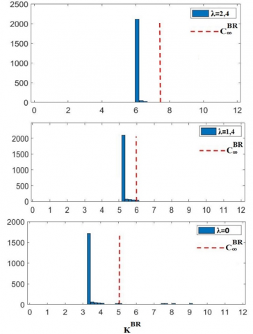
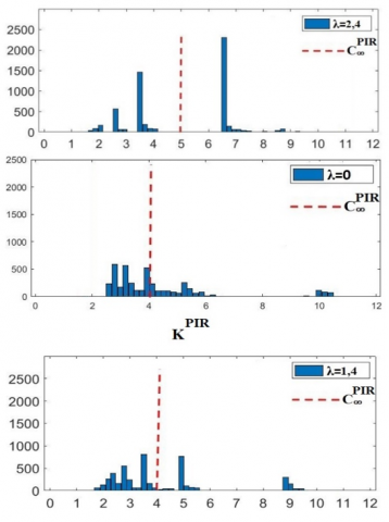
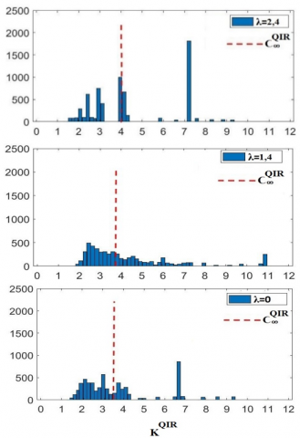
For the second objective, $\lambda$ is set to $2.4,1.4$, and 0 respectively, and the BR, PIR, and QIR strategies are optimized according to criterion (20). The asymptotic average costs $C_{\infty}$ and the histograms of $K$ associated with the optimal configuration of these maintenance strategies are presented in Figure 1.
As $\lambda$ increases, the dispersion of the histogram of $K$ reduces. However, this comes at the cost of a decrease in average economic performance. Table 2 provides a more quantitative result, showing that for all strategies, larger values of $\lambda$ lead to smaller standard deviation $\sigma$ values. This behavior is expected due to the variability of the cost during optimization. A simple adjustment of the value of $\lambda$ allows for the consideration of robustness. However, this may result in a loss of economic performance despite obtaining better robustness of maintenance strategies.
(a) BR strategy
(b) PIR strategy
(c) QIR strategy
Figure 1. MCPRC histogram of BR, PIR and QIR strategies
Table 2. Maintenance strategies optimization of the BR, PIR, and QIR strategies
|
Strategies |
Relative Weight |
Optimal Decision Variables |
Long-Run Expected Cost Rate |
Standard Deviation of MCPRC |
|
BR |
$\lambda=2.4$ |
$T_{\text {opt }}=8.20$ |
$\begin{aligned} & C_{\infty}^{B R}=6.713\end{aligned}$ |
$\begin{aligned} & C_{\infty}^{B R}=3.721\end{aligned}$ |
|
$\lambda=1.4$ |
$T_{\text {opt }}=9.70$ |
$\begin{aligned} & C_{\infty}^{B R}=5.986\end{aligned}$ |
$\begin{aligned} & C_{\infty}^{B R}=4.109\end{aligned}$ |
|
|
$\lambda=0$ |
$T_{\text {opt }}=15.90$ |
$\begin{aligned} & C_{\infty}^{B R}=5.054\end{aligned}$ |
$\begin{aligned} & C_{\infty}^{B R}=5.682\end{aligned}$ |
|
|
PIR |
$\lambda=2.4$ |
$\begin{aligned} & \Delta T_{\text {opt }}=8.29 \\ & M_{\text {opt }}=4.80\end{aligned}$ |
$\begin{aligned} & C_{\infty}^{PIR}=4.982\end{aligned}$ |
$\begin{aligned} & C_{\infty}^{PIR}=4.409\end{aligned}$ |
|
$\lambda=1.4$ |
$\begin{aligned} & \Delta T_{o p t}=6.19 \\ & M_{o p t}=12.8\end{aligned}$ |
$\begin{aligned} & C_{\infty}^{PIR}=4.103\end{aligned}$ |
$\begin{aligned} & C_{\infty}^{PIR}=4.115\end{aligned}$ |
|
|
$\lambda=0$ |
$\begin{aligned} & \Delta T_{o p t}=5.50 \\ & M_{o p t}=16.50\end{aligned}$ |
$\begin{aligned} & C_{\infty}^{PIR}=4.025\end{aligned}$ |
$\begin{aligned} & C_{\infty}^{PIR}=5.009\end{aligned}$ |
|
|
QIR |
$\lambda=2.4$ |
$\begin{aligned} & \alpha_{o p t}=0.37 \\ & M_{o p t}=8.80\end{aligned}$ |
$\begin{aligned} & C_{\infty}^{PIR}=4.063\end{aligned}$ |
$\begin{aligned} & C_{\infty}^{B R}=4.020\end{aligned}$ |
|
$\lambda=1.4$ |
$\begin{aligned} & \alpha_{o p t}=0.55 \\ & M_{o p t}=18.3\end{aligned}$ |
$\begin{aligned} & C_{\infty}^{PIR}=3.832\end{aligned}$ |
$\begin{aligned} & C_{\infty}^{B R}=4.140\end{aligned}$ |
|
|
$\lambda=0$ |
$\begin{aligned} & \alpha_{o p t}=0.34 \\ & M_{o p t}=15.60\end{aligned}$ |
$\begin{aligned} & C_{\infty}^{PIR}=3.667\end{aligned}$ |
$\begin{aligned} & C_{\infty}^{B R}=4.487\end{aligned}$ |
It is also observed that for high values of $\lambda$, the maintenance strategies result in a higher asymptotic average cost per unit of time. Therefore, it can be deduced that robustness and performance may be opposing or even contradictory concepts. Therefore, it is necessary to find a balance between these two factors to improve planning and budget allocation for maintenance activities. A more detailed analysis of this point will be presented in Section 5.
This section presents a comparison study of the BR, PIR, and QIR strategies to evaluate their performance and robustness in different scenarios with varying maintenance cost configurations and relative weight parameter values $(\lambda)$.
The study aims to determine the most suitable maintenance strategy for specific objectives or situations.
By analyzing how the optimal decision variables of these strategies change, we can estimate the settings that work best for them under different combinations of maintenance costs and system characteristics. This guides us in making informed choices regarding maintenance strategies based on our specific needs and circumstances.
5.1 Sensitivity to the maintenance costs
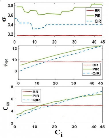
We can identify the best maintenance plans for a given performance and robustness goal thanks to this study. Furthermore, by determining which elements are most important to this goal, we may be able to lessen their detrimental effects. In our system, we keep the CR cost constant at $C_c=98$ and set $\lambda$ to 1.4. Eq. (21) with $C_0=48, M_s$ $=14, \alpha=0.1, \beta=0.1$, and $L=29$ is the PR cost function that we employ. Then, the two configurations for inspection and downtime costs listed below are taken into account:
Keep in mind that maintenance expenses have to meet the restriction $0<C_i<C_p\left(X_t\right)<C_c\left(X_t\right)$.
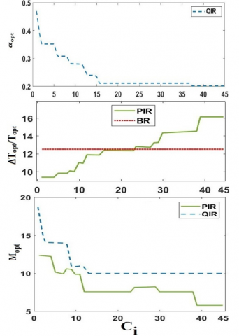
Figures 2(a) and (b), which depict the evolution of the best choice factors and the costs associated with them, are shown in the first case study. Considering that the BR policy does not call for an inspection operation, it is not unexpected that the values of $T_opt$ stay constant with regard to $\mathcal{C}_i$. Nonetheless, because the PIR and QIR policies depend on inspection costs, the fluctuation of $\mathcal{C}_i$ is closely tracked by their optimum decision variables. In order to enable more frequent monitoring of the system's degrading status, Figure 2(b) illustrates how, for the QIR policy, $\alpha$opt is set at a high value and $\Delta T_{\text {opt }}$ of the PIR policy is set at a low value when inspection is affordable. Furthermore, $M_opt$ is set to a high value for both policies in an effort to maximize the system's usable lifespan. The rules reduce the number of inspections by setting $\alpha$opt and $\Delta T_{\text {opt }}$ to higher and lower values, respectively, as inspection costs rise. Because of this, when $\mathcal{C}_i$ rises to extremely high values, the inter-inspection intervals for the PIR and QIR policies are longer than $T_opt$ for the BR policy. In order to reduce system downtime, the ideal PR thresholds $M_opt$ for the PIR and QIR policies are set at a low value, allowing system replacements at the first inspection date. Consequently, Figure 2(a) illustrates how the PIR and QIR policies are most beneficial when $\mathcal{C}_i$ is small and less beneficial when $\mathcal{C}_i$ grows.
(a) Cost functions: $\sigma, \phi_{o p t}$ and $C_{\infty}$
(b) Optimal decision variables: $\alpha_{o p t}, T_{o p t}, \Delta T_{o p t}$ and $M_{o p t}$
Figure 2. Varied inspection cost
(a) Cost functions: $\sigma, \phi_{o p t}$ and $C_{\infty}$
(b) Optimal decision variables: $\alpha_{o p t}, T_{o p t}, \Delta T_{o p t}$ and $M_{o p t}$
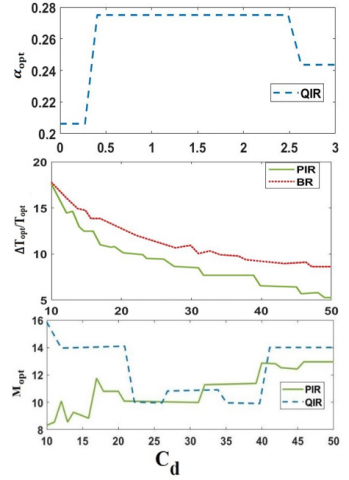
Figure 3. Varied system downtime cost
The reason for the loss is that the PIR and QIR policies have extra inspection procedures that drive up expenses, although they operate identically to the BR policy. The consistency of the MCPRC standard deviations with regard to $C_i$ is demonstrated in Figure 2(a), suggesting that variations in inspection costs have no discernible impact on the resilience of the BR, PIR, or QIR policies. Additionally, whereas these differences are not statistically significant, the MCPRC standard deviations for the CBM policies (PIR and QIR policies) continue to be larger than those for the TBM policy (BR policy). Because of this, CBM policies' decision structures are often weaker than TBM policies'.
On the other hand, they may save more money on upkeep, which would increase their total effectiveness. Selecting the right maintenance structure requires striking a compromise between performance and robustness in maintenance practices.
An effective heuristic for making decisions is the objective function $\varphi$. When $C_i$ is small, the PIR and QIR policies perform better than the BR policy in terms of the objective function $\varphi$; but, when $C_i$ is bigger, they perform worse (see the figure at the top of Figure 2(a)).
The second case study's results are shown in Figure 3. Figures 3(a) and (b) are interpreted similarly to the previous case study.
It is significant to remember that the configuration in the second case study at $C_d=19$ is the same as the setup in the first case study at $C_i=7$. Furthermore, there is an increase in $\alpha_{o p t}$ for the QIR policy. Higher system downtime cost rates $\mathrm{C}_{\mathrm{d}}$ result in large increases in $T_{\text {opt }}$ for BR policies and decreases in $\Delta T_{\text {opt }}$ for PIR policies, respectively, as Figure 3(b) illustrates. Reducing system downtime is the goal of this modification, which will also lower related expenses. The variable evolution of $M_{o p t}$ in PIR and QIR policies implies that the PR threshold here plays a supporting role, essentially acting as an extra regulator to adjust the policies to their ideal setup. It is clear from looking at Figure 3(a) that variations in $C_d$ have a substantial impact on the robustness and performance of the BR, PIR, and QIR policies. Nearly equal long-term projected maintenance cost rates—both lower than the BR policy—are seen in the PIR and QIR policies. For both the BR and QIR strategies, the MCPRC standard deviations are similar. The performance and resilience of the PIR and QIR policies are superior to those of the BR policy. It follows that their performance against the BR policy with respect to the objective cost function $\varphi$ is not surprising (see the upper figure in Figure 3(a)).
Figures 1-3 provide insights into the performance and robustness of different maintenance policies (BR, PIR, and QIR) under varying conditions of maintenance costs and system characteristics. Here's an interpretation of the results and some general guidelines for practitioners:
Figure 1:
Figure 2:
Figure 3:
General Guidelines for Practitioners:
BR Policy:
PIR Policy:
QIR Policy:
Practitioners should consider the specific characteristics of their systems, including maintenance costs, system downtime costs, and the feasibility of inspection operations, to choose the most suitable maintenance policy that balances cost-effectiveness with robustness. Additionally, they should regularly review and adjust maintenance strategies based on changing system conditions and objectives.
5.2 Sensitivity to the relative weight of the cost variability
When choosing a maintenance program, decision-makers' financial prudence and risk tolerance are reflected in the parameter $\lambda$, which stands for relative weight. Quantitatively evaluating the impact of $\lambda$ on the resilience and efficacy of the maintenance solutions under consideration is helpful. In order to do this, we keep the maintenance costs at $C_i=5, C_d=34$, $C_c=98$, and $C_0=48$ and the system characteristics at $\alpha=\beta=$ $0.1, L=29$, and $M_s=14 . \lambda$ was systematically changed throughout the research in increments of 0.1 from 0 to 3 . Figure 4(a) and (b) show the changes in the cost metrics ( $\varphi_{\text {opt }}$, $C_{\infty}$, and $\sigma$ ) and important decision variables ( $T_{o p t}, \Delta T_{o p t}, \alpha_{o p t}$, and $M_{o p t}$ ) for the BR, PIR, and QIR policies, respectively.
(a) Cost functions: $\sigma, \phi_{o p t}$ and $C_{\infty}$
(b) Optimal decision variables: $\alpha_{o p t}, T_{o p t}, \Delta T_{o p t}$ and $M_{o p t}$
Figure 4. Varied relative weight of the cost variability
The robustness of maintenance strategies is gradually prioritized by decision-makers as $\lambda$ rises. Looking at Figure 4(b), we can see that the $T_{\text {opt }}$ of the BR policy goes down, while the $\Delta T_{\text {opt }}$ and $\alpha_{\text {opt }}$ of the PIR and QIR policies stay pretty much the same. On the other hand, $M_{o p t}$, the ideal PR thresholds, tend to fall as $\lambda$ increases. As a result, for CBM policies, the only variables that respond to changes in the relative weight of cost variability $(\lambda)$ are those that are associated with the conditionbased element (i.e., $M_{o p t}$ for PIR and QIR policies). Achieving the right balance between robustness and performance in CBM strategies just requires adjusting these factors.
It is clear from looking at Figure 4(a) that the long-term projected cost rates $\left(C_{\infty}\right)$ and the MCPRC standard deviations $(\sigma)$ for both strategies show different trajectories as a function of $\lambda$. This demonstrates that robustness and performance are fundamentally at odds with one another, making it challenging to get both at the same time. But in terms of the ultimate objective functions ($\varphi_{\text {opt }}$), the QIR policy performs better than the BR and PIR policies, achieving a better compromise between robustness and maintenance performance.
To explore alternative degradation models. Considering different models is crucial for a comprehensive understanding of the subject matter. The modeling approach described in the provided text encompasses several assumptions and limitations that affect its applicability and realism. Let's discuss these limitations, the realism of the Gamma degradation process, and alternative degradation models:
6.1 Limitations and assumptions of the modeling approach
6.2 Realism of the Gamma degradation process
6.3 Alternative degradation models
In conclusion, while the Gamma degradation process and the modeling approach described offer valuable insights, practitioners should be aware of their limitations and consider alternative models and methodologies to enhance the realism and effectiveness of reliability and maintenance modeling in real-world applications. Depending on the specific characteristics of the system and the degradation process under study, alternative models like Weibull distributions, proportional hazard models, or non-parametric approaches may offer more accurate representations and better inform maintenance decision-making.
This study has provided valuable insights into the optimization of maintenance strategies, emphasizing the balance between resilience and performance. Through a quantitative evaluation of three maintenance systems, we have demonstrated the significance of a criterion that aims to achieve the best possible outcome with minimal risk and cost.
Key findings of this research include the superiority of Condition-Based Maintenance (CBM) strategies over Time-Based Maintenance (TBM) methods in terms of economic performance, despite CBM's lower robustness. However, a notable compromise between resilience and performance is observed with CBM, suggesting its practical viability in real-world applications.
Furthermore, the inclusion of system downtime in maintenance expenditures has been identified as a critical factor influencing the resilience of a strategy. The potential of conditional techniques, such as the Quality Improvement Ratio (QIR) method, in mitigating system downtime and enhancing robustness has been highlighted.
The practical implications of these findings are significant for maintenance optimization in various industries. By understanding the trade-offs between robustness and performance, decision-makers can develop more effective maintenance plans that minimize costs while ensuring system reliability. The adoption of CBM strategies, coupled with innovative techniques for managing system downtime, holds promise for achieving optimal maintenance outcomes in practice.
In summary, this paper contributes to the ongoing discourse on maintenance optimization by providing actionable insights and practical recommendations for enhancing resilience and performance in maintenance strategies. These findings have implications for improving asset management practices and ultimately, driving efficiency and sustainability in industrial operations.
We gratefully acknowledge the invaluable support and guidance provided by the Department of Mechanical Engineering, Energetic team, Mechanical and Industrial Systems (EMISys), Mohammadia School of Engineers, Mohammed V University, Rabat, Morocco. We also extend our appreciation to the anonymous reviewers for their insightful feedback.
|
BR |
block replacement strategy |
|
CBM |
condition-based maintenance |
|
$\mathrm{C}_{d}$ |
the system downtime cost rate |
|
$\mathrm{C}_{i}$ |
the inspection cost |
|
$\mathrm{C}_{\infty}$ |
long-run expected maintenance cost rate criterion |
|
$\Delta \mathrm{T}_{\mathrm{opt}}$ |
inter-inspection time between inspections (i) and (i+1) |
|
$\Lambda$ |
relative weight of the cost variability |
|
m |
the average degradation rate |
|
MCPRC |
maintenance cost per renewal cycle |
|
Μopt |
PR threshold (of system state) |
|
PIR |
periodic inspection and replacement strategy |
|
$\varphi$ |
optimal cost function |
|
QIR |
quantile-based inspection and replacement policy |
|
$\sigma$ |
standard deviation of the MCPRC |
|
Topt |
inter-inspection time |
|
TBM |
time-based maintenance |
|
var |
the variance |
[1] Cheikh, K., Boudi, E.M., Rabi, R., Mokhliss, H. (2024). Influence of the relative weight of the performance and robustness of condition-based maintenance strategies and time-based maintenance strategies. Journal of Harbin Engineering University, 45(1): 93-98.
[2] Cheikh, K., Boudi, E.M. (2023). Evaluating the performance and robustness of condition-based maintenance strategies and time-based maintenance strategies. Journal Mechanical Engineering Research and Developments, 46(1): 76-85.
[3] Amari, S.V., McLaughlin, L., Pham, H. (2006). Cost-effective condition-based maintenance using Markov decision processes. In RAMS '06. Annual Reliability and Maintainability Symposium, Newport Beach, CA, USA, pp. 464-469. https://doi.org/10.1109/RAMS.2006.1677417
[4] Asmussen, S. (2003). Applied Probability and Queues (2nd ed.). Applications of Mathematics-Stochastic Modelling and Applied Probability. Springer, 51.
[5] Abate, J., Whitt, W. (1992). The Fourier series method for inverting transforms of probability distributions. Queueing Systems, 10: 5-87. https://doi.org/10.1007/BF01158520
[6] Valdez-Flores, C., Feldman, R.M. (1989). A survey of preventive maintenance models for stochastically deteriorating single-unit systems. Naval Research Logistics (NRL), 36(4): 419-446. https://doi.org/10.1002/1520-6750(198908)36:4%3C419::AID-NAV3220360407%3E3.0.CO;2-5
[7] Scarf, P.A. (2007). A framework for condition monitoring and condition based maintenance. Quality Technology & Quantitative Management, 4(2): 301-312. https://doi.org/10.1080/16843703.2007.11673152
[8] Jardine, A.K.S., Lin, D., Banjevic, D. (2006). A review on machinery diagnostics and prognostics implementing condition-based maintenance. Mechanical Systems and Signal Processing, 20(7): 1483-1510. https://doi.org/10.1016/j.ymssp.2005.09.012
[9] Filar, J.A., Kallenberg, L.C.M., Lee, H.M. (1989). Variance penalized Markov decision processes. Mathematics of Operations Research, 14(1): 147-161. https://doi.org/10.1287/moor.14.1.147
[10] Jeang, A. (1999). Tool replacement policy for probabilistic tool life and random wear process. Quality and reliability engineering international, 15(3): 205-212. https://doi.org/10.1002/(SICI)1099-1638(199905/06)15:3%3C205::AID-QRE244%3E3.0.CO;2-M
[11] Siu, N. (1994). Risk assessment for dynamic systems: An overview. Reliability Engineering & System Safety, 43(1): 43-73. https://doi.org/10.1016/0951-8320(94)90095-7
[12] Grall, A., Dieulle, L., Bérenguer, C., Roussignol, M. (2002). Continuous-time predictive-maintenance scheduling for a deteriorating system. IEEE Transactions on Reliability, 51(2): 141-150. https://doi.org/10.1109/TR.2002.1011518
[13] A-Hameed, M.S., Proschan, F. (1973). Nonstationary shock models. Stochastic Processes and Their Applications, 1(4): 383-404. https://doi.org/10.1016/0304-4149(73)90019-7
[14] Aalen, O.O. (1995). Phase type distribution in survival analysis. Scandinavian Journal of Statistics, 22(4): 447-463.
[15] Abdel-Hameed, M. (2014). Lévy Processes and Their Applications in Reliability and Storage. New York: Springer.
[16] REYNOLDS, John T. Development and Application of API Risk Based Inspection Planning for Petroleum and Petrochemical Facilities. In: ASME International Mechanical Engineering Congress and Exposition. American Society of Mechanical Engineers, 2000. p. 133-144.
https://doi.org/10.1115/IMECE2000-1034
[17] Bagdonavicius, V., Nikulin, M.S. (2001). Estimation in degradation models with explanatory variables. Lifetime Data Analysis, 7: 85-103. https://doi.org/10.1023/A:1009629311100
[18] Meeker, W., Escobar, L. (1998). Statistical Methods for Reliability Data. John Wiley & Sons.
[19] Barlow R.B., Proschan, F. (1975). Statistical Theory of Reliability and Life Testing: Probability Models. Holt, Rinehart and Winston.
[20] Dominguez-Garcia, A.D., Kassakian, J.G., Schindall, J.E., Zinchuk, J.J. (2008). An integrated methodology for the dynamic performance and reliability evaluation of fault-tolerant systems. Reliability Engineering & System Safety, 93(11): 1628-1649. https://doi.org/10.1016/j.ress.2008.01.007
[21] Boursier, J.M., Desjardins, D., Vaillant, F. (1995). The influence of the strain-rate on the stress corrosion cracking of alloy 600 in high temperature primary water. Corrosion Science, 37(3): 493-508. https://doi.org/10.1016/0010-938X(94)00158-3
[22] Dekker, R., Scarf, P.A. (1998). On the impact of optimisation models in maintenance decision making: The state of the art. Reliability Engineering & System Safety, 60(2): 111-119. https://doi.org/10.1016/S0951-8320(98)83004-4
[23] Bond, L.J., Taylor, T.T., Doctor, S.R., Hull, A.B., Malik, S.N. (2008). Proactive management of materials degradation for nuclear power plant systems. In 2008 International Conference on Prognostics and Health Management, Denver, CO, USA, pp. 1-9. https://doi.org/10.1109/PHM.2008.4711466