Fadhil A. Hasan*![]() | Hawraa Q. Hameed
| Hawraa Q. Hameed![]() | Lina J. Rashad
| Lina J. Rashad![]()
© 2024 The authors. This article is published by IIETA and is licensed under the CC BY 4.0 license (http://creativecommons.org/licenses/by/4.0/).
OPEN ACCESS
This paper presents an approach that combines Lyapunov theorem and particle swarm optimization (PSO). The combination tackles the optimization and stability concerns, in controlling permanent magnet synchronous motors (PMSMs). This approach ensures that the exploration is maintained within the search space region, enhances convergence properties, and reduces the risk of divergence or oscillations. This concept is utilized to optimize the field oriented controller (FOC) of PMSM using Matlab Simulink. Each proportional integral (PI) controller in the FOC system is individually optimized using the proposed technique. Simulation results confirm the effectiveness of the proposed method that gave a rise time of 0.71s, an overshoot of 0.04%, and a steady-state time of 0.725s as conjunction to traditional optimization methods. This provides more reliable and efficient frameworks, for solving complicated optimization problems.
Lyapunov theorem, particle swarm optimization (PSO), robust control, PMSM, field oriented control (FOC)
Control Lyapunov functions play a role, in studying the stability and controllability of nonlinear control systems. They can be used to design feedback laws that stabilize the system and also serve as a guarantee for achieving null-controllability as demonstrated by Sontag [1]. Since there is no formulation for a control Lyapunov function in general we have to rely on numerical methods. However common numerical techniques suffer from the curse of dimensionality, which refers to the increase in work as the state dimension grows. In other words, preserving a control Lyapunov function becomes increasingly challenging as the state space dimension increases. Consequently, these techniques are typically limited to low-dimension problems.
The integration of the Lyapunov theorem and the particle swarm optimization (PSO) algorithm represents a dynamic field that has garnered increasing attention in recent years. The roots of Lyapunov-based optimization lie in Aleksandr Lyapunov pioneering work in stability theory during the late 19th century. His theorem, which established criteria for the stability of equilibrium points in dynamical systems, laid the groundwork for stability analysis. Early works like Khalil's "Nonlinear Systems" [2] provided an important connection between stability theory and optimization, setting the stage for subsequent developments. The convergence of the Lyapunov theorem and optimization techniques gained momentum with the emergence of particle swarm optimization. Kennedy and Eberhart's seminal work on PSO [3] marked a significant turning point in the field of optimization, introducing a novel algorithm inspired by social behaviour. As researchers recognized the potential benefits of coupling Lyapunov stability analysis with PSO, a series of theoretical advancements emerged. Sharma et al. [4] proposed a hybrid Lyapunov-fuzzy controller for nonlinear constrained optimization, three variants of the hybrid controller are proposed which are implemented for benchmark simulation and real-life experimentation, the results demonstrate the usefulness of the proposed approach. Lo and Lin [5] present A homogeneously Lyapunov function for an observed-state feedback polynomial fuzzy control system. To verify the proposed method, four examples are demonstrated to show the promising features of the approach adduced. Bhattacharya et al. [6] proposes three alternative extensions to the classical global-best PSO dynamics. Simulation results reveal that the proposed extensions outperform of the classical in terms of convergence speed and accuracy. Cheng et al. [7] proposed an improved sliding mode extremely seeking virtual sensors for the freight train issue of acquiring the optimal creep-speed in real-time, a particle swarm algorithm PSO-based estimation method was presented for the issue of uncertain resistance parameters.
Recent developments in literature have shown a growing interest in approaches that combine PSO with optimization techniques, such as integrating PSO, with Kharitonov’s theorem according to Hasan et al. [8] also merging PSO with Routh Hurwitz’s theory as suggested by Hasan et al. [9]. These combinations show a superior enhancing of the performances of the optimization techniques, in term of computation time, accuracy, and stability. The use of permanent magnet machines shows promise, in achieving high performance. These machines have features such as being lightweight and having power density. One significant advantage is that they produce low levels of noise and vibration compared to machines. This makes them particularly suitable for integration into cars whether it's for in-wheel or in-line configurations [10].
In the field of automation close movement control systems have evolved with controlled motors playing a vital role as core components. As a result, high duty machine control systems are widely used to optimize efficiency in automated manufacturing sectors improving output rates and product quality. However, meeting the criteria for machine speed, efficiency, accuracy, and smoothness largely depends on the motor control techniques.
The robust control of the PMSM is crucial for many operational reasons such as [11, 12]:
Therefore, numerous developed control techniques have been conceived recently to improve the speed control performance of PMSM in various applications. These methods include automatic disturbance rejection control [13], wavelet fuzzy logic control [14], predictive control [15], artificial intelligence-incorporated control [16], sliding mode control [17], and disturbance observer [18]. Furthermore, as an alternative to the traditional PI control, $\mathrm{H} \infty$ control is in operational use. In $\mathrm{H} \infty$ control, exterior disruptions are considered uncertainty parameters within limited boundaries [19]. A robust controller based on hybrid sensitivity can advance the controller for each model in PMSM systems, as in the study [20]. Other efforts have focused on the optimization of the PI controllers with intelligent networks by tuning facilitated to overcome the nonlinear problems [11, 12].
Despite the high performance provided by these methods, they often do not give satisfactory responses in nonlinear systems. The PMSM is considered a highly nonlinear system, as the parameters of the motor and controller are varied with changes in operating conditions, such as temperature, load torque, supplied voltage, etc. Therefore, the proposed method is considered very suitable for controlling nonlinear systems such as PMSM. By leveraging the advantage of the nonlinear optimization capabilities of PSO and stability analysis provided by the Lyapunov theorem, the control method can deal with the inherent nonlinearity of PMSM systems more effectively. In this work, we explore the combination of Lyapunov based stability analysis and particle swarm optimization (PSO) to develop a vector controller, for the permanent magnet synchronous motor (PMSM). Our main focus is on finding values for the parameters of a proportional integral (PI) controller. What sets our approach apart is the use of an objective cost function (CF) that takes into account both dynamic and steady state behaviors. This unique cost function is the contribution of this work, which is characterized by simplicity compared to the complex and sophisticated cost functions presented in previous works. This comprehensive cost function assesses system response by considering constraints for achieving performance. The paper is organized as follows; Section 2 presents an overview of the PMSM while Section 3 provides an introduction to the FOC technique. The optimization algorithm and the chosen cost function are discussed in Sections 4 to 6. We then proceed to present simulation results engage in discussions and draw conclusions.
The Permanent Magnet Motor (PMSM) has only a stator circuit that can be modeled and works within the d-q reference frame. Choosing the rotor reference frame is crucial because it determines the generation of force, stator voltage, and rotor torque, in the machine [21-23].
Before establishing the model we make the assumptions;
These assumptions are essential to eliminate or reduce the complexity associated with certain aspects of the motor, such as magnetic saturation, rotor saliency, or nonlinearities. This reduction in complexity can lead to faster computation times and more straightforward control design. Besides, assumptions can make the mathematical model more efficient in terms of memory and computational resources.
The equations for motor voltage, within the dq model are formulated as follows:
$v_q=R i_q+p \psi_q+\omega_r \psi_d$ (1)
$v_d=R i_d+p \psi_d-\omega_r \psi_q$ (2)
where, $p$ represents the differentiation operator, $R$ is stator resistance, $i_d$ signifies the current in the d-direction current, $\psi_d$ denotes flux in the d-axis, $\psi_q$ represents the flux in the q-axis, $i_q$ symbolizes the current in the q-direction current, and $\omega_r$ signifies rotor angular speed.
The flux linkage is represented as:
$\psi_q=L_q i_q+L_m i_{q r}$ (3)
$\psi_d=L_d i_d+L_m i_{d r}$ (4)
Since the permanent magnet rotor's flux is aligned along the d-axis, the current of the d-axis rotor ($i_{d r}$) remains constant. Simultaneously, the current of the q-axis rotor ($i_{q r}$) is considered negligible due to the absence of rotor flux along this axis.
$\psi_q=L_q i_q$ (5)
$\psi_d=L_d i_d+L_m i_{d r}$ (6)
The linkage flux $\psi_m$ generated by permanent magnets that link the stator is described as:
$\psi_m=L_m i_{d r}$ (7)
The electrical torque is expressed as:
$T_e=\frac{3}{2} * \frac{P}{2} *\left[\psi_m * i_q+\left(L_d-L_q\right) i_q i_d\right]$ (8)
where, $L_d$ and $L_q$ represent d-q inductances, and P signifies the poles number. Both terms in this equation possess physics-based definitions. The "magnet" term of torque is independent of $i_d$ but is directly proportional to $i_q$. This equation underscores that torque hinges on rotor type, inductance values ($L_d, L_q$), and rotor permanent magnets. For the PMSM, surface-mounted rotor magnets render the reluctance term irrelevant, as $L_d$ equal $L_q$. On the other hand, when permanent magnets are placed in the inner side, the rotor's saliency leads to a disparity between $L_d$ and $L_q$ [21].
The electromagnetic torque is formulated as:
$T_e=\frac{3}{2} * \frac{P}{2} * \psi_m * i_q$ (9)
Given that magnetic flux linkage remains constant, torque is directly proportional to the q-axis current.
The electromagnetic torque equation can be represented as:
$T_e=T_L+B \omega_r+J \frac{d \omega_r}{d t}$ (10)
In this equation, $T_L$ signifies the load torque, B represents the viscous friction coefficient, $\omega_r$ is the rotor angular speed, and J is the rotor's moment of inertia.
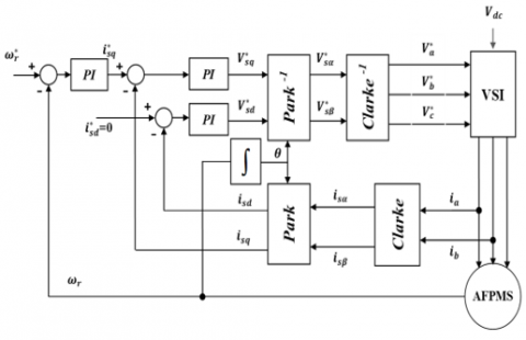
Field oriented control, also known as "decoupling control" divides the stator current of a three phase motor into two components. One component generates the flux while the other produces torque. This approach enables control over both flux and torque making it possible to compare magnet synchronous motors (PMSMs) with separately excited DC machines. By employing FOC, as shown in Figure 1, which laniaries the PMSM model due, to the nonlinear relationships, between flux linkages, inductor currents and rotor angle we can effectively mitigate any nonlinearity.
Figure 1. Block diagram of the field oriented control
FOC is widely used in PMSM drive systems where a modulation current is injected into the motor windings to induce a rotating flux that propels the rotor. The vector control technique is implemented within a rotating reference frame. Field oriented control can be implemented using either a direct or an indirect approach.
In PMSM systems the vector control technique is preferred for its simplicity, implementation, operational robustness and clear guidelines compared to PI controller strategies.
Moreover, field oriented control provides benefits including responsiveness, minimal fluctuation, in torque and straightforward integration. In practice the PI controller is commonly employed for computing flux, torque and speed [23, 24].
Particle swarm optimization (PSO) is an optimization technique inspired by the movement patterns of birds and fish. It was first introduced in 1995 by Kennedy and Eberhart. PSO involves particles moving within a population guided by their best positions ($p_{{best }}$) and the most favorable global position, in the current generation ($g_{{best }}$) [3]. Mathematically, we can represent the speed and location of a particle as follows:
$\begin{gathered}\hat{v}_j(k)=W \cdot \hat{v}_j(k-1)+\beta_1 \cdot \mathbb{R}_1 \cdot\left(p_{\text {best }_j}(k)-\bar{\chi}_j(k-1)\right) +\beta_2 \cdot \mathbb{R}_2 \cdot\left(g_{\text {best } j}(k)-\bar{\chi}_j(k-1)\right)\end{gathered}$ (11)
$\bar{\chi}_j(k)=\bar{\chi}_j(k-1)+\hat{v}_j(k)$ (12)
where,
$\hat{v}_j(k)=\left[\hat{v}_{j 1}(k) \hat{v}_{j 2}(k) \ldots \hat{v}_{j n}(k)\right]$ is an n-dimensional speed vector at iteration k.
$\bar{\chi}_j(k)=\left[\bar{\chi}_{j 1}(k) \bar{\chi}_{j 2}(k) \ldots \bar{\chi}_{j n}(k)\right]$ is an n-dimensional the location vector at iteration k.
$p_{ {best } j}(k)=\left[p_{ {best } j 1}(k) p_{ {best } j 2}(k) \ldots p_{{best } j n}(k)\right]$ is an n-dimensional vector of the local best position at iteration k.
$g_{ {best } j}(k)=\left[g_{ {best } j 1}(k) g_{ {best } j 2}(k) \ldots g_{ {best } j n}(k)\right]$ is an n-dimensional vector of the global best position at iteration k.
$\beta_1$ stands for capabilitys learning swiftness, $\beta_2$ denotes effect and $\left[\mathbb{R}_1, \mathbb{R}_2\right]$ are random values, within the range of [0, 1], W refers to the learning weighted coefficient.
The optimization steps can be summarized in the following algorithm:
Begin
Initializing parameters;
While iteration not reaches end Do
{
For j = 1 to no. of particles
{
Estimate cost function CF(j)of particle j;
If CF($\bar{\chi}_j$)<CF($p_{ {bestj} }$) Then Update local location;
}; // End for
Update global location; // by Min.(CF(all best locals)
Update speed (Eq.11);
Update locations (Eq. 12);
}; //End while;
End
Lyapunov theory handles the stability of equilibrium points in dynamic systems. The stability threshold is a condition at which the system stays unaffected over time. The technique concentrates on deciding whether the equilibrium point is stable or unstable and whether the system converges to a precise state as time progresses.
5.1 Formal statement of Lyapunov theorem
Lyapunov theorem can be stated as follows:
Consider a system described by the differential equation
$\begin{gathered}\dot{x}=G(x)=g(x, r(x)) \\ x \in \mathcal{R}^n ; r \in \mathcal{R}^m \\ \dot{x}(0)=G(0)=g(0, r(0))=0\end{gathered}$ (13)
where, x represents the state variables and $\dot{x}$ denotes their derivatives with respect to time. If there exists a continuously differentiable function $G(x)$, known as a Lyapunov function. The process of finding Lyapunov functions lacks a standardized approach; sometimes, they emerge as natural energy functions for mechanical or electrical systems, while other times, their discovery relies on a process of trial and error [2]. Converse Lyapunov theorems establish that the presence of a Lyapunov function is synonymous with asymptotic stability [25].
The function $\mathcal{H}(x)$ is deemed a Lyapunov function if there is a region in the vicinity of the origin where:
1. $\mathcal{H}(x)$ is positive definite (i.e., $\mathcal{H}(x)$ > 0 for all x except at the equilibrium point itself).
2. The time derivative of $\dot{\mathcal{H}}(x)$ along the trajectories of the system, $\dot{\mathcal{H}}(x)=\frac{\partial \mathcal{H}(x)}{\partial t}$, is negative definite (i.e., $\dot{\mathcal{H}}(x)$< 0 for all x except at the equilibrium point).
3. Also, $\mathcal{H}(x) \dot{\mathcal{H}}(x)<0$
This area is referred to as the region of attraction.
$\dot{\mathcal{H}}(x)=\nabla \mathcal{H}(x) G(x)=\sum_{i=1}^n \frac{\partial \mathcal{H}}{\partial x_i} g_i(x)$ (14)
where,
$\nabla \mathcal{H}(x)=\left[\frac{\partial \mathcal{H}(x)}{\partial x_1}, \frac{\partial \mathcal{H}(x)}{\partial x_2}, \ldots, \frac{\partial \mathcal{H}(x)}{\partial x_n}\right]$ (15)
The Lyapunov stability theorem asserts that if $\dot{x}$ possesses the origin as an equilibrium point and there exists a suitable Lyapunov function $\mathcal{H}(x)$ satisfying $\mathcal{H}(0)=0$ and $\mathcal{H}(x)>0$ for all $x \neq 0$, as well as $\dot{\mathcal{H}}(x) \geq 0$ for all x, then the origin is stable. Furthermore, if $\mathcal{H}(x)<0$ for all $x \neq 0$, the origin is globally asymptotically stable [2]. The choice of a Candidate Lyapunov Function is such that $\mathcal{H}(x)$ is continuously differentiable and positive definite. Stability is ensured if $\mathcal{H}(x)$ is positive definite and $\dot{\mathcal{H}}(x)$ is negative definite for all $x \in \mathcal{R}^n$ [2, 21].
5.2 Lyapunov function of the PMSM
The primary control objective is torque control. Consequently, it is imperative to minimize both the $i_d$ and $i_q$ errors, in addition to the speed error, down to zero. Upon examining the small-scale dynamic model, it becomes evident that the load torque term in Eq. (10) is nullified. The Lyapunov function can be extracted from Eq. (1), Eq. (2) and Eq. (10) as follows:
By setting:
$\left[\begin{array}{l}x_1 \\ x_2 \\ x_3\end{array}\right]=\left[\begin{array}{l}i_d \\ i_q \\ \omega_r\end{array}\right] ;\left[\begin{array}{l}u_1 \\ u_2 \\ u_3\end{array}\right]=\left[\begin{array}{l}v_d \\ v_q \\ T_e\end{array}\right]$
Then
$\dot{x_1}=-\frac{R}{L_d\left(x_1\right)} x_1+P \frac{L_q\left(x_2\right)}{L_d\left(x_1\right)} x_2 x_3+u_1 \frac{1}{L_d\left(x_1\right)}$ (16)
$\begin{gathered}\dot{x_2}=-\frac{R}{L_q\left(x_2\right)} x_2-P \frac{L_d\left(x_1\right)}{L_q\left(x_2\right)} x_1 x_3 -P \frac{\psi_m}{L_q\left(x_2\right)} x_3+u_2 \frac{1}{L_q\left(x_2\right)}\end{gathered}$ (17)
$\dot{x_3}=-\frac{B}{J} x_3-\frac{T_L}{J}+u_3 \frac{1}{J}$ (18)
where, $x_1, x_2$, and $x_3$ are the state variables and $u_1, u_2$, and $u_3$ are the control signals.
Considering the electromagnetic torque expression given in Eq. (8), it becomes evident that achieving torque control is attainable through the closed-loop regulation of $i_d$ and $i_q$ currents. In the case of motors with surface magnets, the relationship between torque and $i_d$ is straightforward. However, for motors with interior magnets, this connection involves both $i_d$ and $i_q$, rendering it more intricate. The designed control system is tailored to accomplish the objective of torque tracking. The input voltages are devised in a manner that ensures the convergence of ($i_d$ and $i_q$) to their desired trajectory ($i_d^*$ and $i_q^*$). Given that $i_d^*=0$, the desired electromagnetic torque is directly proportional to the desired current $i_q^*$.
In pursuit of the currents tracking objective, the tracking errors are defined as:
$\begin{gathered}\varepsilon_d=i_d^*-i_d=x_1^*-x_1=-x_1 \\ \varepsilon_q=i_q^*-i_q=x_2^*-x_2 \\ \varepsilon_\omega=\omega_r^*-\omega_r=x_3^*-x_3\end{gathered}$ (19)
Then the dynamic change in errors can by driven from Eq. (16), Eq. (17) and Eq. (18) as:
$\begin{gathered}\dot{\varepsilon_d}=-\frac{u_1}{L_d}+\frac{R}{L_d} x_1-\frac{L_q}{L_d} x_2 x_3 \\ \dot{\varepsilon_q}=-\frac{u_2}{L_q}+\frac{R}{L_q} x_2-\frac{L_d}{L_q} x_1 x_3+\frac{\psi_m}{L_q} x_3 \\ \dot{\varepsilon_\omega}=-\frac{u_3}{J}+\frac{T_L}{J}+\frac{B}{J} x_3\end{gathered}$ (20)
To guarantee the convergence of the tracking errors towards zero, the selected Lyapunov function is formulated as:
$\begin{gathered}\mathcal{H}(x)=\frac{1}{2} \delta_1 \Theta_d^2+\frac{1}{2} \varepsilon_d^2+\frac{1}{2} \delta_2 \Theta_q^2+\frac{1}{2} \varepsilon_q^2 \\ +\frac{1}{2} \delta_3 \Theta_\omega^2+\frac{1}{2} \varepsilon_\omega^2\end{gathered}$ (21)
where, $\Theta_d=\int_0^t \varepsilon_d(\tau) d \tau$, $\Theta_q=\int_0^t \varepsilon_q(\tau) d \tau$, and $\Theta_\omega=\int_0^t \varepsilon_\omega(\tau) d \tau$ are the integral time error (ITE) of the dq-currents and speed, $\delta_1, \delta_2$, and $\delta_3$ are positive real constants.
Incorporating these integral actions into the Lyapunov function ensures the achievement of tracking error convergence to zero, even in the presence of system disturbances and model uncertainties. Utilizing Eq. (14) and Eq. (15), the derivative of the Lyapunov function can be computed as follows:
$\begin{gathered}\dot{\mathcal{H}}(x)=\varepsilon_d\left(\delta_1 \Theta_d-\frac{u_1}{L_d}+\frac{R}{L_d} x_1-\frac{L_q}{L_d} x_2 x_3\right) \\ +\varepsilon_q\left(\delta_2 \Theta_q-\frac{u_2}{L_q}+\frac{R}{L_q} x_2+\frac{L_d}{L_q} x_1 x_3+\frac{\psi_m}{L_q} x_3\right) \\ +\varepsilon_\omega\left(\delta_\omega \Theta_\omega-\frac{u_3}{J}+\frac{T_L}{J}+\frac{B}{J} x_3\right)\end{gathered}$ (22)
Now, based on Eq. (22), the stability of the system can be proved as following:
To ensure global asymptotic stability within the current loop, the synthesis of d-q axes controllers must keep $\mathcal{H}(x)$ as positive definite and $\dot{\mathcal{H}}(\mathrm{x})$ as negative definite for all values of the state variables $x$. Obviously, Eq. (22) consists of three terms; the first term represents the stability criteria of the d-axis current control loop, and the second term represents the stability criteria of the q-axis current control loop. While, the third term represents the stability criteria of the speed control loop.
The integration of the Lyapunov theorem with particle swarm optimization (PSO) has been identified in existing literature as an intricate implementation strategy and a sophisticated methodology, as evidenced by references [4] and [6]. However, in the present study, a more streamlined approach has been adopted to synergize these concepts.
Combining PSO with the Lyapunov theorem leverages the strengths of both techniques to achieve optimal, stable, adaptive, and robust control solutions for complex nonlinear systems. Thus, the choice of the cost function must involve all those constraints. Besides, obtaining a powerful cost function must prevent the algorithm from falling in local optima, divergence, or oscillation. Thus, the chosen cost function was formulated to evaluate those approaches. The optimization process entails the selection of a cost function, achieved through the multiplication of two distinct sub-cost functions: $\eta\left(k_{i, j}\right)$ and $\xi\left(k_{i, j}\right)$ each of which encapsulates pertinent characteristics delineated by their respective functions. The first sub-cost function $\eta\left(k_{i, j}\right)$ represents the dynamic and steady-state response which consists of a summation of three constraints:
$\begin{gathered}\eta\left(k_{i, j}\right)=\min \left\{\left|\frac{O S^*-O S\left(k_{i, j}\right)}{O S^*}\right|+\left|\frac{T_r^*-T_r\left(k_{i, j}\right)}{T_r^*}\right|\right. \left.+\operatorname{ITSE}\left(k_{i, j}\right)\right\}\end{gathered}$ (23)
where, $O S^*$ and $O S\left(k_{i, j}\right)$ are the maximum allowable and currently overshoot respectively, $T_r^*$ and $T_r\left(k_{i, j}\right)$ are the required and actual rise time respectively, and $\operatorname{ITSE}\left(k_{i, j}\right)$ corresponds to the integral-time square speed error. The ITSE reflects a steady-state error, while overshoot and rise time pertain to transient response. The optimization technique's goal is to minimize this sub-cost function and improve both transient and steady-state performance.
The second sub-cost function $\xi\left(k_{i, j}\right)$ operates as a discerning indicator by actively assessing whether the system violates the prescribed Lyapunov stability criteria, as defined in Eq. (22), throughout each iterative cycle. This evaluative process can be succinctly encapsulated within a conditional construct (if statement), thereby elucidating instances where deviations from the established stability parameters manifest.
$\xi\left(k_{i, j}\right)=\left\{\begin{array}{lr}1 & \text { if } \dot{\mathcal{H}}(x) \leq 0 \\ 10^6 & \text { if } \dot{\mathcal{H}}(x)>0\end{array}\right.$ (24)
If the optimization process applied individually for the three controllers Eq. (22) can be eliminated to on term that represents that specific control.
The cost function is
$C F\left(k_{i, j}\right)=\eta\left(k_{i, j}\right) * \xi\left(k_{i, j}\right)$ (25)
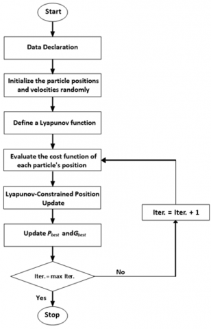
Figure 2. Flowchart of the optimization process
The central idea of incorporating Lyapunov theorem into PSO lies in utilizing Lyapunov functions to define and maintain a stable region within the search space. This approach ensures that particles not only explore the search space for optimal solutions but also remain within a region that guarantees stability. Figure 2 summarized the optimization algorithm flowchart.
The simulation configuration includes the FOC approach executed within a d-axis and q-axis model based on a decoupled method. To connect the motor with the controller, the dq-abc and abc-dq transformations are utilized. A driving voltage source inverter is blended into the system to control the PMSM using a 600V DC link. The machine parameters which used in the simulation are summarized in Table 1. These parameters play important functions in performing the motor's behaviour and characteristics. The particle swarm optimization algorithm was integrated within the Lyapunov concepts by sub-Matlab routines, assisting in the evaluation of optimal control parameters. The overall system was simulated providing a reliable representation of how the different components interact and affect the comprehensive behaviour of the PMSM under control.
The optimization PSO process is executed with the following parameter values: $\beta_1=\beta_2=1.5$, W=0.7 and a total of 100 iterations are performed. These parameters are crucial in determining the balance between exploration and exploitation of the solution space. The dynamic response boundaries are chosen as $O S^*=1 \%$ and $T_r^*=1 \mathrm{~s}$ as maximum allowable.
Table 1. Parameter values of the PMSM
|
Parameters |
Physical Meaning |
Value |
|
Ld (mH) |
q-axis inductance |
1.5 |
|
Lq (mH) |
d-axis inductance |
1.5 |
|
Rs (Ω) |
Armature winding resistance |
0.13 |
|
J (kg.m2) |
Rotor moment of inertia |
0.1 |
|
P |
Machine pole pairs |
6 |
|
$\psi_m$ (Wb) |
Permanent pole magnetic flux |
0.028 |
Table 2 provides an overview of the resultant parameters for the three PI controllers after the optimization process. These controllers play a pivotal role in the FOC strategy, influencing the motor's performance and response characteristics.
Table 2. Optimal controllers’ gains
|
Controller |
Kp |
Ki |
|
Speed |
9.82 |
14.4 |
|
q-axis current |
1.03 |
10.8 |
|
d-axis current |
2.34 |
6.5 |
The results depicted in Figure 3 illustrate the tendency of particles within the state space, concentrating towards the global optimum solution. Sealed red particles are the banned particles that guide toward unstable reactions during optimization. The reached values of particles, after 100 iterations, characterize the optimal parameters of the system controllers. Figure 4 represents the track of the cost function throughout the optimization procedure. The CF values change as the optimization algorithm progresses, showcasing the iterative performance improvement.
Figure 3. Particles convergence toward the global optima
Figure 4. Trajectory of the CF toward minimum value
Figure 5. Step response performances
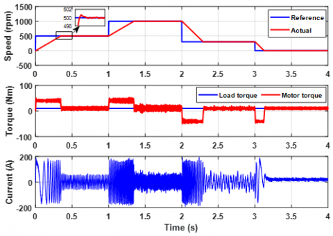
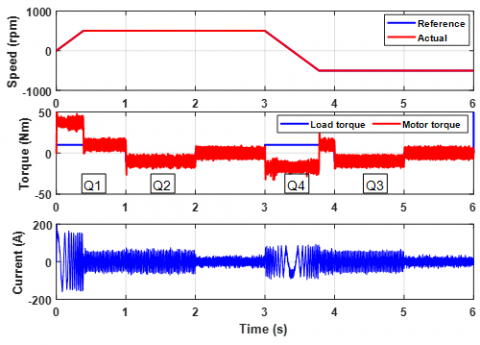
Figure 5 shows the system's performance evaluated for varying step commands in speed tracking. This figure provides insights into how well the system responds to different reference speed changes. Figure 6 shows the acceleration and deceleration performance in four-quadrant operating modes the graph demonstrates the system's response to ramp commands. It provides a comprehensive view of how the system handles dynamic changes in speed commands. Figure 7 investigates the d-axis and q-axis stator currents concerning variations in speed and torque. It validates the precision of the FOC technique and its ability to adapt to changing operating conditions.
Figure 6. Four-quadrant operation
Figure 7. dq-axis currents performance
Furthermore, to assess the robustness of the suggested controllers, the deviation of stator resistance and inductance are inspected. The investigation involves analyzing the behaviour of the motor's speed and torque under varying stator parameters. This experimentation provides insights into how well the proposed controller can maintain performance in the presence of parameter variations.
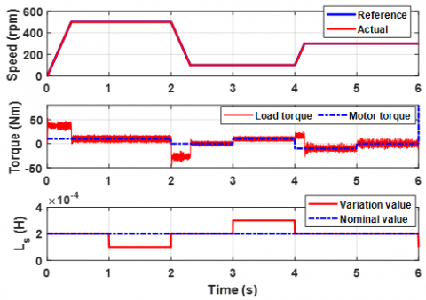
In real-world operational scenarios, various factors such as temperature fluctuations, operating duty cycles, and instances of overloading can impact motor performance. Among these factors, the parameters most susceptible to change are the resistance and inductance of the stator winding. Variations in these parameters lead to degrading the performance which requires robust control techniques. Figure 8 depicts the system's performance in responding to stator resistance variation.
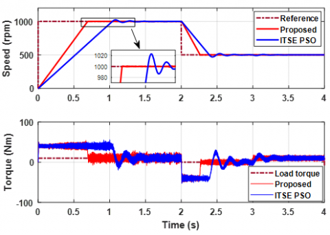
Figure 9 shows the system's behaviour in responding to variations in stator inductance. This demonstrates how the proposed controller can overcome the variation in machine parameters. To evaluate the effectiveness of the proposed controller in conjunction with conventional methods, a comparative investigation is achieved. Specifically, a comparison is made between the proposed controller and an optimized PIPSO controller employing only the Integral-Time Square Error (ITSE) objective function.
Figure 8. Stator resistance variations
Figure 9. Stator inductance variations
Figure 10. Comparison performances
This comparison provides insights into how well the proposed method performs in comparison to a benchmark approach. Figure 10 presents a side-by-side comparison of the performance achieved by the suggested method and the PI-PSO optimization technique that considers only the ITSE fitness function. The graph visually highlights the differences in performance outcomes.
Table 3 summarizes the performance constraints achieved by both the suggested controller and the optimization technique focusing on ITSE. The comparison highlights the improvements achieved by the proposed controller in terms of rise time $T_r$, overshoot $O S$, and steady-state time $T_{s s}$. These results underscore the effectiveness of the multi-objective cost function utilized in the proposed method.
Table 3. Comparison constants
|
Constraints |
ITSE |
Proposed |
|
$T_r$ (s) |
0.95 |
0.71 |
|
$O S$ % |
1.89 |
0.04 |
|
$T_{S S}$ (s) |
2.04 |
0.725 |
In summary, the discussed parameter variation analysis and comparative investigation further validate the robustness and superiority of the proposed controller in enhancing the performance of the PMSM under various operational conditions.
The simulation results affirm the efficacy of the suggested optimization strategy using the cost function incorporated with Lyapunov theorem. The convergence of particles towards optimal values is illustrated in Figure 3 and Figure 4, indicating the validity of the suggested multi-objective cost function. This outcome is obtained by attracting particles towards optimal values using Lyapunov-based constraints; the algorithm guides particles toward regions that enhance convergence properties. The proposed multi-objective cost function contributes to an expedited optimization process by considering transient, steady-state, and stable performance and accommodating multiple constraints. This key contribution distinguishes this work from previous studies that solely employed the ITSE cost function. Figure 5 and Figure 6 demonstrate the PMSM's ramp and step response performance in reference tracking for various input references speed, illustrating excellent operation under full-load conditions. The obtained response parameters, including $T_r$=0.71s, $O S$=0.04%, and steady-state time $T_{s s}$=0.725s, indicate highly satisfactory performance. Furthermore, the robustness of the controllers is exhibited through the investigation of stator parameters. Figure 8 and Figure 9 showcase the system's performance under stator resistance and inductance variations confirm the controller's resilience against parameter changes. The comparison performance presented in Figure 10 confirms the superiority of the proposed controller approach with that employs only the ITSE objective function. This demonstrates the significance of the proposed Lyapunov-base PSO cost function, which enhance the performance as well as integrates: rise time, overshoot, steady-state error, and stability constraints into a single cost function.
This work suggests a combination of Lyapunov-based stability analysis and PSO. To state the benefits of the new optimization method, an optimum controller was designed for speed control of the PMSM. The new approach distinguishes itself from previous works by presenting a comprehensive evaluation of the system's performance. This evaluation process applies a multi-objective cost function that considers steady-state, dynamic, and stability performance. The adopted FOC technique proves its effectiveness in controlling speed and torque control. The optimization algorithm fine-tunes the optimum controller gains, resulting in excellent system performance in speed and torque tracking various operating cases. The simulation outcomes substantiate the efficacy of the suggested cost function in different operating conditions, yielding a rise time of 0.71s, an overshoot of 0.04%, and a steady-state time of 0.725s. Additionally, the proposed controller showcases notable robustness against variations in the machine parameters. However, it's crucial to acknowledge that the rotor torque ripple is considerably significant, potentially leading to undesired operating characteristics. The approach presented in this paper holds promise for advancing the performance of PMSM applications, especially in the context of electric vehicles and other propulsion systems.
The contribution and potential impact of this work can be listed as:
Furthermore, this work can be extended as future aspects can be done in several ways to enhance its effectiveness or address specific challenges:
[1] Sontag, E.D. (1983). A Lyapunov-like characterization of asymptotic controllability. SIAM Journal on Control and Optimization, 21(3): 462-471. https://doi.org/10.1137/0321028
[2] Khalil, H.K. (2002). Nonlinear Systems. 3rd Edition, Prentice Hall, Upper Saddle River.
[3] Kennedy, J., Eberhart, R. (1995). Particle swarm optimization. In Proceedings of ICNN'95 - International Conference on Neural Networks, Perth, WA, Australia, pp. 1942-1948. https://doi.org/10.1109/ICNN.1995.488968
[4] Sharma, K.D., Chatterjee, A., Rakshit, A. (2009). A hybrid approach for design of stable adaptive fuzzy controllers employing Lyapunov theory and particle swarm optimization. IEEE Transactions on Fuzzy Systems, 17(2): 329-342. https://doi.org/10.1109/TFUZZ.2008.2012033
[5] Lo, J.C., Lin, C. (2017). Polynomial fuzzy observed-state feedback stabilization via homogeneous Lyapunov methods. IEEE Transactions on Fuzzy Systems, 26(5): 2873-2885. https://doi.org/10.1109/TFUZZ.2017.2786211
[6] Bhattacharya, S., Konar, A., Das, S., Han, S. Y. (2009). A Lyapunov-based extension to particle swarm dynamics for continuous function optimization. Sensors, 9(12): 9977-9997. https://doi.org/10.3390/s91209977
[7] Cheng, X., He, J., Zhang, C.F., Huang, G., Huang, Y.S. (2022). Adhesion control for freight train based on improved sliding mode extremum seeking algorithm and barrier Lyapunov function. Journal Européen des Systèmes Automatisés, 55(2): 189-196. https://doi.org/10.18280/jesa.550205
[8] Hasan, F.A., Humod, Abdulrahim T., Rashad, Lina J. (2020). Robust decoupled controller of induction motor by combining PSO and Kharitonov’s theorem. Engineering Science and Technology, an International Journal, 23(6): 1415-1424, https://doi.org/10.1016/j.jestch.2020.04.004
[9] Hasan, F.A., Rashad, L.J., Humod, A.T. (2020). Integrating particle swarm optimization and routh-Hurwitz's theory for controlling grid-connected LCL-filter converter. International Journal of Intelligent Engineering & Systems, 13(4): 102-113. https://doi.org/10.22266/ijies2020.0831.10
[10] Patil, N.J., Waghmare, L.M. (2010). Fuzzy adaptive controllers for speed control of PMSM drive. International Journal of Computer Applications, 975: 8887.
[11] Salih, A M., Humod, A.T., Hasan, F.A. (2019). Optimum design for PID-ANN controller for automatic voltage regulator of synchronous generator. In 2019 4th Scientific International Conference Najaf (SICN), Al-Najef, Iraq, pp. 74-79. https://doi.org/10.1109/SICN47020.2019.9019367
[12] Salman, S.S., Humod, A T., Hasan, F.A. (2022). Optimum control for dynamic voltage restorer based on particle swarm optimization algorithm. Indonesian Journal of Electrical Engineering and Computer Science, 26(3): 1351-1359. https://doi.org/10.11591/ijeecs.v26.i3.pp1351-1359
[13] Pyrkin, A., Vedyakov, A., Bobtsov, A., Bazylev, D., Sinetova, M., Ovcharov, A., Vladislav, A. (2020). Adaptive full state observer for nonsalient PMSM with noised measurements of the current and voltage. IFAC-PapersOnLine, 53(2): 1652-1657. https://doi.org/10.1016/j.ifacol.2020.12.2224
[14] Liu, S., Guo, X., Zhang, L. (2017). Robust adaptive backstepping sliding mode control for six-phase permanent magnet synchronous motor using recurrent wavelet fuzzy neural network. IEEE Access, 5: 14502-14515. https://doi.org/10.1109/ACCESS.2017.2721459
[15] Liu, X., Zhang, Q. (2019). Robust current predictive control-based equivalent input disturbance approach for PMSM drive. Electronics, 8(9): 1034. https://doi.org/10.3390/electronics8091034
[16] Jie, H., Zheng, G., Zou, J., Xin, X., Guo, L. (2020). Adaptive decoupling control using radial basis function neural network for permanent magnet synchronous motor considering uncertain and time-varying parameters. IEEE Access, 8: 112323-112332. https://doi.org/10.1109/ACCESS.2020.2993648
[17] Mohd Zaihidee, F., Mekhilef, S., Mubin, M. (2019). Robust speed control of PMSM using sliding mode control (SMC)—A review. Energies, 12(9): 1669. https://doi.org/10.3390/en12091669
[18] De Soricellis, M., Da Ru, D., Bolognani, S. (2017). A robust current control based on proportional-integral observers for permanent magnet synchronous machines. IEEE Transactions on Industry Applications, 54(2): 1437-1447. https://doi.org/10.1109/TIA.2017.2772171
[19] Lee, H., Lee, Y., Shin, D., Chung, C.C. (2015). H∞ control based on LPV for load torque compensation of PMSM. In 2015 15th International Conference on Control, Automation and Systems (ICCAS), Busan, Korea (South), pp. 1013-1018. https://doi.org/10.1109/ICCAS.2015.7364794
[20] Yang, J., Fa, N., Chen, R. (2006). H∞ robust controller based on local feedback recurrent neural network for permanent magnet linear synchronous motor. In 2006 CES/IEEE 5th International Power Electronics and Motion Control Conference, Shanghai, China, pp. 1-5. https://doi.org/10.1109/IPEMC.2006.4778191
[21] Krishnan, R. (2001). Electric Motor Drives: Modelling, Analysis, and Control. Prentice-Hall, Upper Saddle River.
[22] Lian, J., Xie, S., Jian, W., Hu, P. (2012). Nonlinear model of permanent-magnet synchronous motors. International Journal of Digital Content Technology and its Applications, 6(7): 119-126. https://doi.org/10.4156/jdcta.vol6.issue7.15
[23] Jash, K., Saha, P.K., Panda, G.K. (2013). Vector control of permanent magnet synchronous motor based on sinusoidal pulse width modulated inverter with proportional integral controller. International Journal of Engineering Research and Applications, 3(5): 913-917.
[24] Bida, V.M., Samokhvalov, D.V., Al-Mahturi, F.S. (2018). PMSM vector control techniques—A survey. In 2018 IEEE Conference of Russian Young Researchers in Electrical and Electronic Engineering (EIConRus), Moscow and St. Petersburg, Russia, pp. 577-581. https://doi.org/10.1109/EIConRus.2018.8317164
[25] EI Idrissi, A.E.J., Beniysa, M., Bouajaj, A., Britel, M.R. (2021). Intelligent control of uncertain PMSM based on stable and adaptive discrete-time neural network compensators. Journal Européen des Systèmes Automatisés, 54(4): 575-589. https://doi.org/10.18280/jesa.540407