Le Van Anh![]() | Vu Thi To Linh*
| Vu Thi To Linh*![]()
© 2024 The authors. This article is published by IIETA and is licensed under the CC BY 4.0 license (http://creativecommons.org/licenses/by/4.0/).
OPEN ACCESS
Overhead cranes are used to move heavy, bulky objects above the factory floor instead of along floor walkways. They are commonly used to load and unload goods in factories, outdoor warehouses and serve at stations, ports. During operation, chain hoists or cable hoists are the main equipment, plays the role of hoisting/lowering materials and moving mechanism along the main beam. Therefore, vibration cannot be avoided during the process of moving heavy objects, causing danger to people and affecting the product. In addition, the overhead crane is an uncertain nonlinear system, compared to the single pendulum type, moving two loads at the same time is much more complicated. That's why the author proposes to design a new controller that not only helps balance the cart but also the two pendulums during operation. First, the system dynamics model is built. Next, an adaptive controller based on the radial basis function neural network (RBFNN) is designed and proven to be stable according to Lyapunov theory. Simulation results of the overhead crane system on MATLAB/Simulink software have shown the effectiveness of the proposed algorithm even when the working system is affected by model uncertainty.
overhead crane, radial basis function neural network, adaptive control, Lyapunov theory
Overhead crane is a type of equipment used to lift and move goods in factories as well as outdoors. Normally, overhead cranes are often used in factories, but when used outdoors, people use gantry cranes. The use of overhead cranes is very convenient and highly effective in work, loading and unloading goods and bulky heavy objects such as iron and steel in steel factories. Operated mainly by electric motors, it is widely used in industrial plants, steel plants, hydroelectric plants, as well as civil works...
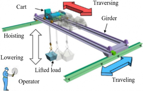
The main parts of the overhead crane are shown in detail in Figure 1.
Main beams: These are beams that span the width of the overhead crane and support the moving hoist system. In a single girder overhead crane there is one main girder, while in a double girder overhead crane there are two.
Edge beam: This is a beam frame with wheels located at both ends. They allow the overhead crane to move along the runway beam.
Rail support beams: These are parallel overhead structural beams on which the edge beams move. They will support the entire overhead crane system and are often mounted on support columns or attached to the house frame structure.
(a) Structure of the overhead crane
(b) Operating principle of each part
Figure 1. Structure diagram and operating principle of the overhead crane
Hoist: A hoist is a device that lifts, lowers and holds loads. It can be electric, hand-pulled or pneumatic. Includes motor, gearbox, cable reel, cable or chain and hook.
Cart: The cart is the part that carries the hoist and allows the hoist to move along the main beam. It includes frame, wheels and transmission mechanism.
Control: Overhead cranes can be controlled by wire control, remote control or cabin control. These systems allow operators to control overhead crane movements including hoisting, lowering and positioning loads.
Electrical system: This system includes power supply components such as wires, contact brushes, power rails that supply power to the motor and overhead crane control system.
These parts are shown in detail in Figure 1.
During overhead crane operation, the goal is to design the controller so that the goods are transported to the desired location without vibration or vibration. Usually, parameters such as cable length and load volume change, these are uncertain parameters of the overhead crane. In addition, the system is also affected by external disturbances such as friction, wind... which also make it difficult for the vehicle to reach the desired position and causes the pendulum to vibrate. Therefore, designing a controller for the overhead crane system to ensure stable working system in all situations is always of interest to research by scientists.
In the studies [1, 2], the authors proposed a closed-loop feedback system control structure using a proportional integral derivative (PID) controller to control the position of the cart and reduce the vibration angle. The results show good control performance, fast response, but traditional PID controllers easily lose control when noise occurs, and adjustment depends on the operating engineer. Linear quadratic regulation (LQR) optimal controller proposed in studies [3, 4]. When the system has uncertain model parameters, adaptive control methods have been proposed by authors in the studies [5-12]. A robust control method based on sliding mode control (SMC) is also often applied to nonlinear systems, which is very useful for overhead crane systems [13-16]. However, SMC has disadvantages that cause chattering, affecting output response performance as well as reducing the lifespan of the devices. Model predictive control (MPC) is studied for its advantages in handling constraints as shown in the studies [17, 18]. In addition to the above methods, many intelligent controllers such as fuzzy control [19, 20], neural networks [21, 22] have also been proposed to implement for overhead crane systems.
From the analysis of the works published above, we see that most of these methods only design control for structural systems with one load. For a system consisting of two loads, research mainly proposes traditional control methods and represents the model in linear form. Therefore, the authors proposed an adaptive control method based on the RBF neural network for the uncertain nonlinear overhead crane system.
In summary, the main contributions of this paper are presented in the following ideas.
- Designing a new controller not only helps balance the cart but also helps balance the two pendulums during operation.
- The effects of model uncertainty are regulated by an adaptive law based on the RBF neural network. This is completely suitable for real-life applications when overhead cranes operate.
- Data about overhead crane systems can be measured through output feedback, reducing costs when designing hardware.
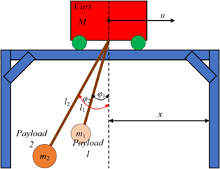
We can represent a simple model of a crane system as shown in Figure 2. Suppose the cart, pendulum and payload work on a two-dimensional plane, the cart moves on a horizontal line.
Figure 2. Simple overhead crane system model
The overhead crane system model can be built according to the Newton-Euler or Euler-Lagrange method. In this study, the authors use the Euler-Lagrange method based on kinetic and potential energy to establish the equations of the mechanical system. The Euler-Lagrange equation is represented as follows:
$\frac{d}{d t}\left(\frac{\partial L}{\partial \dot{q}}\right)-\frac{\partial L}{\partial q}+\frac{\partial P}{\partial q}=u$ (1)
where, $L$ and $P$ are kinetic energy and potential energy, respectively; $u$ denotes the driving force of the cart; $q=$ $\left[\begin{array}{lll}x & \varphi_1 & \varphi_2\end{array}\right]^T, x$ is the position of the cart, $\varphi_1$ and $\varphi_2$ are the positions of pendulum 1 and pendulum 2 , respectively, relative to the vertical axis.
The total potential energy of the mechanical system is written as:
$\begin{gathered}P=m_1 l_1 g\left(1-\cos \left(\varphi_1(t)\right)\right) +m_2 l_2 g\left(1-\cos \left(\varphi_2(t)\right)\right)\end{gathered}$ (2)
The total kinetic energy of a mechanical system is written as:
$\begin{gathered}L=\frac{1}{2} m_1 v_1^2+\frac{1}{2} m_2 v_2^2+\frac{1}{2} M \dot{x}^2 =\frac{1}{2} m_1\left(\left(l_1 \dot{\varphi}_1 \sin \varphi_1\right)^2+\left(\dot{x}-l_1 \dot{\varphi}_1 \cos \varphi_1\right)^2\right) +\frac{1}{2} m_2\left(\left(l_2 \dot{\varphi}_2 \sin \varphi_2\right)^2+\left(\dot{x}-l_2 \dot{\varphi}_2 \cos \varphi_2\right)^2\right) +\frac{1}{2} M \dot{x}^2\end{gathered}$ (3)
where, $\dot{x}$ is the linear velocity of the cart; $\dot{\varphi}_1$ is the angular velocity of the payload $1 ; \dot{\varphi}_2$ is the angular velocity of the payload $2 ; v_1, v_2$ are the velocity components of the pendulum in the $\mathrm{x}$ and $\mathrm{y}$ directions calculated as follows:
$v_1^2=\left(\dot{x}-l_1 \dot{\varphi}_1 \cos \varphi_1\right)^2+\left(l_1 \dot{\varphi}_1 \sin \varphi_1\right)^2 ;$
$v_2^2=\left(\dot{x}-l_2 \dot{\varphi}_2 \cos \varphi_2\right)^2+\left(l_2 \dot{\varphi}_2 \sin \varphi_2\right)^2$.
The parameters of the mechanical system model are described in Table 1.
Table 1. Parameters of the mechanical system model
|
Symbol |
Meaning |
|
$M$ |
Denotes the mass of the cart |
|
$m_1$ |
Mass of payload 1 |
|
$l_1$ |
Cable length between the center of the cart and the payload 1 |
|
$\varphi_1$ |
Payload 1 swing angle |
|
$m_2$ |
Mass of payload 2 |
|
$l_2$ |
Cable length between the center of the cart and the payload 2 |
|
$\varphi_2$ |
Payload 2 swing angle |
|
g |
Gravitational constant |
Partial derivative of Eq. (1) with respect to the variables $x, \varphi_1, \varphi_2$ respectively.
Partial derivative with respect to variable x we get:
$\begin{gathered}\frac{d}{d t}\left(\frac{\partial L}{\partial \dot{x}}\right)-\frac{\partial L}{\partial x}+\frac{\partial P}{\partial x}=u \\ \Rightarrow m_1 l_1\left(\dot{\varphi}_1^2 \sin \varphi_1-\ddot{\varphi}_1 \cos \varphi_1\right) \\ +m_2 l_2\left(\dot{\varphi}_2^2 \sin \varphi_2-\ddot{\varphi}_2 \cos \varphi_2\right) \\ +\left(m_1+m_2+M\right) \ddot{x}=u \\ \Rightarrow \ddot{x}=\frac{m_1 l_1\left(\ddot{\varphi}_1 \cos \varphi_1-\dot{\varphi}_1^2 \sin \varphi_1\right)}{m_1+m_2+M} \\ +\frac{m_2 l_2\left(\ddot{\varphi}_2 \cos \varphi_2-\dot{\varphi}_2^2 \sin \varphi_2\right)}{m_1+m_2+M}+\frac{u}{m_1+m_2+M}\end{gathered}$ (4)
Partial derivative with respect to variable $\varphi_1$ we get:
$\begin{gathered}\frac{d}{d t}\left(\frac{\partial L}{\partial \dot{\varphi}_1}\right)-\frac{\partial L}{\partial \varphi_1}+\frac{\partial P}{\partial \varphi_1}=0 \\ \Rightarrow m_1 l_1\left(g \sin \varphi_1-\cos \varphi_1 \ddot{x}+l_1 \ddot{\varphi}_1\right)=0 \\ \left(g \sin \varphi_1-\cos \varphi_1 \ddot{x}+l_1 \ddot{\varphi}_1\right)=0 \\ \Rightarrow \ddot{\varphi}_1=\frac{\cos \varphi_1 \ddot{x}-g \sin \varphi_1}{l_1}\end{gathered}$ (5)
Similarly, partial derivative with respect to variable $\varphi_2$ we have:
$\begin{gathered}\frac{d}{d t}\left(\frac{\partial L}{\partial \dot{\varphi}_2}\right)-\frac{\partial L}{\partial \varphi_2}+\frac{\partial P}{\partial \varphi_2}=0 \\ \Rightarrow m_2 l_2\left(g \sin \varphi_2-\cos \varphi_2 \ddot{x}+l_2 \ddot{\varphi}_2\right)=0 \\ \left(g \sin \varphi_2-\cos \varphi_2 \ddot{x}+l_2 \ddot{\varphi}_2\right)=0 \\ \Rightarrow \ddot{\varphi}_2=\frac{\cos \varphi_2 \ddot{x}-g \sin \varphi_2}{l_2}\end{gathered}$ (6)
Substituting Eqs. (6) and (5) into Eq. (4) we have:
$\begin{aligned} \ddot{x}= & \frac{-m_1 g \sin \varphi_1 \cos \varphi_1-m_2 g \sin \varphi_2 \cos \varphi_2}{m_1 \sin ^2\left(\varphi_1\right)+m_2 \sin ^2\left(\varphi_2\right)+M} \\ & +\frac{-m_1 l_1 \dot{\varphi}_1^2 \sin \varphi_1-m_2 l_2 \dot{\varphi}_2^2 \sin \varphi_2}{m_1 \sin ^2\left(\varphi_1\right)+m_2 \sin ^2\left(\varphi_2\right)+M} \\ & +\frac{u}{m_1 \sin ^2\left(\varphi_1\right)+m_2 \sin ^2\left(\varphi_2\right)+M}\end{aligned}$ (7)
Let $X=\left[\begin{array}{llllll}x_1 & x_2 & x_3 & x_4 & x_5 & x_6\end{array}\right]^T$. Then the state space equation of the nonlinear system is:
$\left\{\begin{array}{c}\dot{x}_1=\dot{x}=x_2 \\ \dot{x}_2=\ddot{x}=f_1(X)+g_1(X) u \\ \dot{x}_3=x_4=\dot{\varphi}_1 \\ \dot{x}_4=\ddot{\varphi}_1=f_2(X)+g_2(X) u \\ \dot{x}_5=x_6=\dot{\varphi}_2 \\ \dot{x}_6=\varphi_2=f_3(X)+g_3(X) u\end{array}\right.$ (8)
Eq. (8) is briefly written as follows:
$\dot{X}=F(X)+G(X) u$ (9)
3.1 Adaptive RBFNN controller
Recently, the RBF neural network has attracted the research attention of scientists. With a simple three-layer structure including input layer, hidden layer, output layer and good generalization ability, lengthy and unnecessary calculations are avoided compared to multi-layer feed forward networks.
This section introduces an adaptive control method based on neural approximation with unknown parameters [21-23].
Defining error vector
$e(t)=\left[\begin{array}{c}x_1-x_{\text {ref }} \\ x_3-\varphi_{1 r e f} \\ x_5-\varphi_{2 r e f}\end{array}\right]=\left[\begin{array}{c}x-x_{\text {ref }} \\ \varphi_1-\varphi_{1 r e f} \\ \varphi_2-\varphi_{2 r e f}\end{array}\right]=q-q_{\text {ref }}$ (10)
where, $q_{\text {ref }}=\left[\begin{array}{lll}x_{\text {ref }} & \varphi_{1 \text { ref }} & \varphi_{2 r e f}\end{array}\right]^T, x_{\text {ref }}$ is the desired position and $\varphi_{1 r e f}, \varphi_{2 \text { ref }}$ are the desired rotation angles.
The control law is designed as follows:
$u=\frac{1}{G(X)}\left[\ddot{q}_{r e f}-F(X)+K^T \mathrm{e}\right]$ (11)
where, $e=\left[\begin{array}{ll}e \,\, \dot{e}\end{array}\right]^T, K=\left[\begin{array}{ll}K_p \,\, K_d\end{array}\right]^T$.
Substituting Eq. (11) into (9), we get the error equation of the system as follows:
$\ddot{e}+K_d \dot{e}+K_p e=0$ (12)
We have the characteristic equation of the system as:
$s^2+K_d s+K_p=0$ (13)
where, $K_p$ and $K_d$ are designed so that the characteristic Eq. (13) has a solution on the left side of the complex plane, meaning when $t \rightarrow \infty$ then $e(t) \rightarrow 0$ and $\dot{e}(t) \rightarrow 0$.
To find the control law in Eq. (10), we need to know the function $F(X)$. However, $F(X)$ is an uncertain nonlinear function. Therefore, the authors use the RBFNN to approximate $F(X)$.
The RBFNN is described as follows:
$h_j=\exp \left(\frac{\left\|\mathrm{e}-c_{i j}\right\|^2}{b_j^2}\right)$ (14)
$F(X)=W^T h(e)+\varepsilon$ (15)
where, e is the input vector of the neural network;
i represents the number of input layer neurons;
j represents the number of hidden layer neurons;
$h=\left[h_1, h_2, h_3, \ldots, h_n\right]^T$ represents the output of the hidden layer;
$c_{i j}$ represents the coordinate vector of the center point of the Gaussian basis function;
$b_j$ represents the width of the Gaussian function;
W is the weight value of the neural network;
$\varepsilon$ is the approximation error of the neural network.
Then the function F(X) is approximated as follows:
$\hat{F}(X)=\widehat{W}^T h(e)$ (16)
where, $\hat{F}(X)$ is the output of the neural network; $\hat{W}$ is an approximation of the neural network weight $W$; input vector of the neural network $e=\left[\begin{array}{ll}e \,\, \dot{e}\end{array}\right]^T$.
At this point, the control law (11) will become:
$u=\frac{1}{G(X)}\left[\ddot{q}_{\text {ref }}-\hat{F}(X)+K^T e\right]$ (17)
Substituting Eq. (16) into (17), the system control law is expressed as follows:
$u=\frac{1}{G(X)}\left[\ddot{q}_{r e f}-\widehat{W}^T h(\mathrm{e})+K^T e\right]$ (18)
The neural network weight adaptation law is chosen as:
$\widehat{W}=-\gamma e^T P b h(e)$ (19)
where, P is a positive definite symmetric matrix; $\gamma>0$.
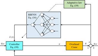
The block diagram of the closed-loop control system is shown in Figure 3.
Figure 3. Block diagram of closed loop control system
3.2 Stability analysis
Substituting Eq. (11) into (9) we have:
$\ddot{e}=(\hat{F}(X)-F(X))-K^T e$ (20)
Transforming Eq. (20) we have:
$\dot{e}=A \mathrm{e}+B(\hat{F}(X)-F(X))$ (21)
Assuming W is the optimal weight of RBFNN, then W is calculated according to the following equation.
$W^*=\operatorname{argmin}(\sup |\hat{F}(X)-F(X)|)$ (22)
Set the model approximation error calculated by the optimal RBFNN weights to be:
$\tilde{F}(X)=\hat{F}\left(X / W^*\right)-F(X)$ (23)
$\Rightarrow \tilde{F}(X)-\hat{F}\left(X / W^*\right)=-F(X)$ (24)
Substituting Eq. (24) into (21) we have:
$\dot{e}=A \mathrm{e}+B\left(\hat{F}(X)+\tilde{F}(X)-\hat{F}\left(X / W^*\right)\right)$ (25)
$\begin{gathered}\Rightarrow \dot{e}=A e+B\left(\hat{F}(X)+\tilde{F}(X)-\hat{F}\left(X / W^*\right)\right) \\ =A e+B\left[\left(\hat{F}(X)-\hat{F}\left(X / W^*\right)\right)\right]+\tilde{F}(X) \\ =A e+B\left(\left(\widehat{W}-W^*\right) h(e)+\tilde{F}(X)\right)\end{gathered}$ (26)
Set $N=B\left(\left(\widehat{W}-W^*\right)^T h(e)+\tilde{F}(X)\right)$, then Eq. (26) is rewritten as:
$\dot{e}=A \mathrm{e}+N$ (27)
Choose the Lyapunov function:
$L=\frac{1}{2} e^T P e+\frac{1}{2 \gamma}\left(\widehat{W}-W^*\right)^T\left(\widehat{W}-W^*\right)$ (28)
The matrix P must satisfy the Lyapunov equation:
$P A+A^T P=-Q$ (29)
where, $A=\left[\begin{array}{cc}0 & I \\ -K_p & -K_d\end{array}\right] ; B=\left[\begin{array}{l}0 \\ I\end{array}\right] ; Q \geq 0$.
$\begin{gathered}\dot{L}=\frac{1}{2} \dot{e}^T P e+\frac{1}{2} e^T P \dot{e}+\frac{1}{\gamma}\left(\widehat{W}-W^*\right)^T \dot{\hat{W}} \\ =\frac{1}{2}\left(e^T A^T+N^T\right) P e+\frac{1}{2} e^T P(A E+N) \\ \quad+\frac{1}{\gamma}\left(\widehat{W}-W^*\right)^T \dot{\hat{W}} \\ =\frac{1}{2} e^T\left(A^T P+P A\right) e+\frac{1}{2} N^T P e+\frac{1}{2} e^T P N \\ \quad+\frac{1}{\gamma}\left(\widehat{W}-W^*\right)^T \dot{\hat{W}} \\ =-\frac{1}{2} e^T Q e+\frac{1}{2}\left(N^T P e+e^T P N\right) \\ \quad+\frac{1}{\gamma}\left(\hat{W}-W^*\right)^T \dot{\hat{W}}\end{gathered}$ (30)
$\Rightarrow \dot{L}=-\frac{1}{2} e^T Q e+e^T P N+\frac{1}{\gamma}\left(\widehat{W}-W^*\right)^T \dot{\hat{W}}$ (31)
Substituting the N value set above into Eq. (31), we get:
$\begin{gathered}\dot{L}=-\frac{1}{2} e^T Q e+e^T P B\left(\left(\widehat{W}-W^*\right)^T h(e)+\tilde{F}(X)\right) \\ +\frac{1}{\gamma}\left(\widehat{W}-W^*\right)^T \dot{\hat{W}} \\ =-\frac{1}{2} e^T Q e+e^T P B\left(\widehat{W}-W^*\right)^T h(e)+e^T P B \tilde{F}(X) \\ +\frac{1}{\gamma}\left(\widehat{W}-W^*\right)^T \dot{\hat{W}} \\ \dot{L}=-\frac{1}{2} e^T Q e+e^T P B \tilde{F}(X) \\ +\frac{1}{\gamma}\left(\widehat{W}-W^*\right)^T\left(\dot{\hat{W}}+\gamma e^T P B h(e)\right)\end{gathered}$ (32)
With the adaptation law Eq. (19) the Lyapunov function becomes:
$\dot{L}=-\frac{1}{2} e^T Q e+e^T P B \tilde{F}(X) \leq 0$ (33)
Complete proof.
To verify the effectiveness of the proposed algorithm. We perform system simulation on Matlab/Simulink software with different scenarios. The selected RBF neural network has 6 input layer neurons, 13 hidden layer neurons and 1 output layer neuron. The hidden layer parameters $c_{i j}$ and $b_j$ of the neural network are: [-3, -2.5, -2, -1.5, -1, -0.5, 0, 0.5, 1, 1.5, 2, 2.5, 3] and 2.
The parameters of the selected controller are: $K_p=30, K_d=50, \gamma=500$. The initial neural network weight values are 0.
Scenario 1: The parameters of the overhead crane system are: $\begin{aligned} M=1000(\mathrm{~kg}), m_1=50(\mathrm{~kg}), m_2=100(\mathrm{~kg}), l_1=10(\mathrm{~m}), l_2=20(\mathrm{~m}) \end{aligned}$.
The initial and desired positions of the system are:
$\left\{\begin{array}{c}X_0=\left[\begin{array}{llllll}3 & 0 & \pi / 3 & 0 & -\pi / 3 & 0\end{array}\right]^T \\ X_{\text {ref }}=\left[\begin{array}{llllll}5 & 0 & 0 & 0 & 0 & 0\end{array}\right]^T\end{array}\right.$
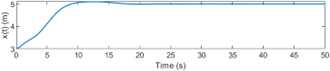
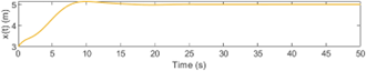
The simulation results from Figures 4-19 show that the proposed controller stabilizes all responses of the overhead crane system with good control performance. The responses of the cart's position and the cable's swing angle always track the set value with a small response time.
Figure 4. Scenario 1 cart position when $x=5$
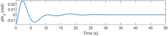
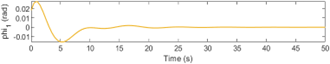
Figure 5. Scenario 1 swing angle of load 1 when $\varphi_1=\pi / 3$
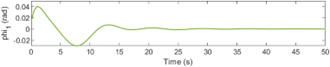
Figure 6. Scenario 1 swing angle of load 2 when $\varphi_2=-\pi / 3$
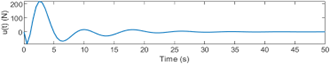
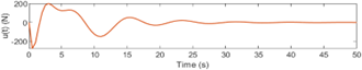
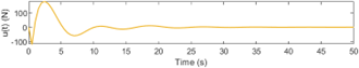
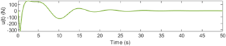
Figure 7. Scenario 1 control input when $x=5$
The initial and desired positions of the system are:
$\left\{\begin{array}{c}X_0=\left[\begin{array}{llllll}5 & 0 & \pi / 4 & 0 & -\pi / 4 & 0\end{array}\right]^T \\ X_{\text {ref }}=\left[\begin{array}{llllll}10 & 0 & 0 & 0 & 0 & 0\end{array}\right]^T\end{array}\right.$
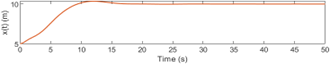
Figure 8. Scenario 1 cart position when $x=10$
Figure 9. Scenario 1 swing angle of load 1 when $\varphi_1=\pi / 4$
Figure 10. Scenario 1 swing angle of load 2 when $\varphi_2=-\pi / 4$
Figure 11. Scenario 1 control input when $x=10$
Scenario 2: The parameters of the overhead crane system are: $\begin{aligned} M=100(\mathrm{~kg}), m_1=5(\mathrm{~kg}), m_2=10(\mathrm{~kg}), l_1=1(\mathrm{~m}), l_2=2(\mathrm{~m}) \end{aligned}$.
The initial and desired positions of the system are:
$\begin{gathered}X_0=\left[\begin{array}{llllll}3 & 0 & \pi / 3 & 0 & -\pi / 3 & 0\end{array}\right]^T \\ X_{\text {ref }}=\left[\begin{array}{llllll}5 & 0 & \pi / 3 & 0 & -\pi / 3 & 0\end{array}\right]^T\end{gathered}$
Figure 12. Scenario 2 cart position when $x=5$
Figure 13. Scenario 2 swing angle of load 1 when $\varphi_1=\pi / 3$
Figure 14. Scenario 2 swing angle of load 2 when $\varphi_2=-\pi / 3$
Figure 15. Scenario 2 control input when $x=5$
The initial and desired positions of the system are:
$\left\{\begin{array}{c}X_0=\left[\begin{array}{llllll}5 & 0 & \pi / 4 & 0 & -\pi / 4 & 0\end{array}\right]^T \\ X_{\text {ref }}=\left[\begin{array}{llllll}10 & 0 & 0 & 0 & 0 & 0\end{array}\right]^T\end{array}\right.$
Figure 16. Scenario 2 cart position when $x=10$
Figure 17. Scenario 2 swing angle of load 1 when $\varphi_1=\pi / 4$
Figure 18. Scenario 2 swing angle of load 2 when $\varphi_2=-\pi / 4$
Figure 19. Scenario 2 control input when $x=10$
The simulation results from Figures 4-19 show that the proposed controller stabilizes all responses of the overhead crane system with good control performance. The responses of the cart's position and the cable's swing angle always track the set value with a small response time.
The adaptability of the controller is studied in relation to changes in the parameters of the overhead crane system. Usually the volume of the load is very diverse and depends on each individual operating condition. By varying the mass of the load and the cable length, we obtain the system response as shown in Figures 12-19. Note that the controller parameters remain the same in the two scenarios.
The results obtained with the controller using RBF neural network (overshoot 0.217%) show that the system quality is improved in terms of overshoot compared to the fuzzy logic controller [24] (overshoot 0.227%). In addition, fuzzy logic controllers have the disadvantage of depending on the expert's understanding of the object. Specifically, the operating range of input and output variables needs to be surveyed first because they greatly affect the quality of the system when using a fuzzy logic controller.
In this study, the authors have transformed the dynamic equation of the overhead crane system in accordance with the proposed control method. The proposed controller is stable for all outputs of the system: the position of the cart and the rotation angle of the cable accurately track the desired values, the vibration of the goods is completely suppressed. The adaptability of the system is guaranteed when changing the system parameters to suit the reality when the crane operates. Finally, in the near future the author will conduct experiments to check the simulation results.
A potential future research direction is to install the algorithm on real application systems. In addition, we need to integrate additional obstacle avoidance features into the controller to ensure safety for people and goods during operation.
This study was supported by University of Economics - Technology for Industries (UNETI), Ha Noi – Viet Nam; Website: http://www.uneti.edu.vn/.
|
M |
Denotes the mass of the cart, kg |
|
$m_1$ |
Mass of payload 1, kg |
|
$l_1$ |
Cable length between the center of the cart and the payload 1, m |
|
$m_2$ |
Mass of payload 2, kg |
|
$l_2$ |
Cable length between the center of the cart and the payload 2, m |
|
g |
Gravitational constant, m/s2 |
|
e |
The input vector of the neural network |
|
i |
Represents the number of input layer neurons |
|
j |
Represents the number of hidden layer neurons |
|
h |
Represents the output of the hidden layer |
|
$c_{i j}$ |
Represents the coordinate vector of the center point of the Gaussian basis function |
|
$b_ j$ |
Represents the width of the Gaussian function |
|
W |
The weight value of the neural network |
|
X |
State space variables |
|
Greek symbols |
|
|
$\varphi_1$ |
Payload 1 swing angle, rad |
|
$\varphi_2$ |
Payload 2 swing angle, rad |
|
$\varepsilon$ |
The approximation error of the neural network |
|
Subscripts |
|
|
ref |
reference |
[1] Fantuzzi, N., Rustico, A., Formenti, M., Ferreira, A.J. (2022). 3D active dynamic actuation model for offshore cranes. Computer-Aided Civil and Infrastructure Engineering, 37(7): 864-877. https://doi.org/10.1111/mice.12690
[2] Vaughan, J., Karajgikar, A., Singhose, W. (2011). A study of crane operator performance comparing PD-control and input shaping. In Proceedings of the 2011 American Control Conference, San Francisco, CA, USA, pp. 545-550. https://doi.org/10.1109/ACC.2011.5991506
[3] Yang, B., Xiong, B. (2010). Application of LQR techniques to the anti-sway controller of overhead crane. Advanced Materials Research, 139: 1933-1936. https://doi.org/10.4028/www.scientific.net/amr.139-141.1933
[4] Jafari, J., Ghazal, M., Nazemizadeh, M. (2014). A LQR optimal method to control the position of an overhead crane. IAES International Journal of Robotics and Automation, 3(4): 252.
[5] Sun, N., Fang, Y., Chen, H. (2015). Adaptive antiswing control for cranes in the presence of rail length constraints and uncertainties. Nonlinear Dynamics, 81(1-2), 41-51. https://doi.org/10.1007/s11071-015-1971-y
[6] Ouyang, H., Tian, Z., Yu, L., Zhang, G. (2020). Adaptive tracking controller design for double-pendulum tower cranes. Mechanism and Machine Theory, 153: 103980. https://doi.org/10.1016/j.mechmachtheory.2020.103980
[7] Abdullahi, A.M., Mohamed, Z., Selamat, H., Pota, H.R., Abidin, M.Z., Ismail, F.S., Haruna, A. (2018). Adaptive output-based command shaping for sway control of a 3D overhead crane with payload hoisting and wind disturbance. Mechanical Systems and Signal Processing, 98: 157-172. https://doi.org/10.1016/j.ymssp.2017.04.034
[8] Sun, N., Yang, T., Chen, H., Fang, Y., Qian, Y. (2017). Adaptive anti-swing and positioning control for 4-DOF rotary cranes subject to uncertain/unknown parameters with hardware experiments. IEEE Transactions on Systems, Man, and Cybernetics: Systems, 49(7): 1309-1321. https://doi.org/10.1109/tsmc.2017.2765183
[9] Ouyang, H., Wang, J., Zhang, G., Mei, L., Deng, X. (2019). Novel adaptive hierarchical sliding mode control for trajectory tracking and load sway rejection in double-pendulum overhead cranes. IEEE Access, 7: 10353-10361. https://doi.org/10.1109/access.2019.2891793
[10] Zhang, M., Ma, X., Rong, X., Tian, X., Li, Y. (2016). Adaptive tracking control for double-pendulum overhead cranes subject to tracking error limitation, parametric uncertainties and external disturbances. Mechanical Systems and Signal Processing, 76: 15-32. https://doi.org/10.1016/j.ymssp.2016.02.013
[11] He, W., Zhang, S., Ge, S.S. (2013). Adaptive control of a flexible crane system with the boundary output constraint. IEEE Transactions on Industrial Electronics, 61(8): 4126-4133. https://doi.org/10.1109/tie.2013.2288200
[12] Wang, Y., Chen, J., Yan, F., Zhu, K., Chen, B. (2019). Adaptive super-twisting fractional-order nonsingular terminal sliding mode control of cable-driven manipulators. ISA transactions, 86: 163-180. https://doi.org/10.1016/j.isatra.2018.11.009
[13] Li, X., Geng, Z., Peng, X. (2018). A double-sliding surface based control method for underactuated cranes. In 2018 37th Chinese Control Conference (CCC), Wuhan, China, pp. 2648-2652. https://doi.org/10.23919/ChiCC.2018.8483857
[14] Yang, C., Du, C., Liao, L. (2022). Design and implementation of finite time sliding mode controller for fuzzy overhead crane system. ISA Transactions, 124: 374-385. https://doi.org/10.1016/j.isatra.2019.11.037
[15] Wang, T., Tan, N., Zhang, X., et al. (2021). A time-varying sliding mode control method for distributed-mass double pendulum bridge crane with variable parameters. IEEE Access, 9: 75981-75992. https://doi.org/10.1109/access.2021.3079303
[16] Wu, X., Xu, K., Lei, M., He, X. (2020). Disturbance-compensation-based continuous sliding mode control for overhead cranes with disturbances. IEEE Transactions on Automation Science and Engineering, 17(4): 2182-2189. https://doi.org/10.1109/tase.2020.3015870
[17] Chen, H., Fang, Y., Sun, N. (2016). A swing constraint guaranteed MPC algorithm for underactuated overhead cranes. IEEE/ASME Transactions on Mechatronics, 21(5): 2543-2555. https://doi.org/10.1109/tmech.2016.2558202
[18] Wu, Z., Xia, X., Zhu, B. (2015). Model predictive control for improving operational efficiency of overhead cranes. Nonlinear Dynamics, 79: 2639-2657. https://doi.org/10.1007/s11071-014-1837-8
[19] Sun, Z., Bi, Y., Zhao, X., Sun, Z., Ying, C., Tan, S. (2018). Type-2 fuzzy sliding mode anti-swing controller design and optimization for overhead crane. IEEE Access, 6: 51931-51938. https://doi.org/10.1109/access.2018.2869217
[20] Leite, D., Aguiar, C., Pereira, D., Souza, G., Škrjanc, I. (2019). Nonlinear fuzzy state-space modeling and lmi fuzzy control of overhead cranes. In 2019 IEEE International Conference on Fuzzy Systems (FUZZ-IEEE), New Orleans, LA, USA, pp. 1-6. https://doi.org/10.1109/FUZZ-IEEE.2019.8858968
[21] Chen, Q., Cheng, W., Gao, L., Fottner, J. (2021). A pure neural network controller for double-pendulum crane anti-sway control: Based on Lyapunov stability theory. Asian Journal of Control, 23(1): 387-398. https://doi.org/10.1002/asjc.2226
[22] Yang, T., Sun, N., Chen, H., Fang, Y. (2019). Neural network-based adaptive antiswing control of an underactuated ship-mounted crane with roll motions and input dead zones. IEEE Transactions on Neural Networks and Learning Systems, 31(3): 901-914. https://doi.org/10.1109/tnnls.2019.2910580
[23] Qiu, Y., Cai, B., Cui, G. (2020). Research on suspension control strategy based on adaptive RBF neural network for MVAWT. In 2020 Chinese Automation Congress (CAC), Shanghai, China, pp. 1029-1034. https://doi.org/10.1109/CAC51589.2020.9326947
[24] Esleman, E.A., Önal, G., Kalyoncu, M. (2021). Optimal PID and fuzzy logic based position controller design of an overhead crane using the Bees Algorithm. SN Applied Sciences, 3(10): 811. https://doi.org/10.1007/s42452-021-04793-0