Aya M. Hameed* | Ahmed K. Hamoudi
© 2023 IIETA. This article is published by IIETA and is licensed under the CC BY 4.0 license (http://creativecommons.org/licenses/by/4.0/).
OPEN ACCESS
This paper focuses on designing several controllers to attenuate the chattering problem: a conventional sliding mode controller (CSMC) with a barrier function (BF) and a saturation function (SF), and an adaptive sliding mode controller (ASMC) with SF as well as ASMC with BF. The key distinction between CSMC and ASMC lies in the fact that ASMC doesn’t require knowledge of the upper bounds of uncertainties and the determination of gain. ASMC can minimize the magnitude of control signals to an acceptably low level. Despite perturbations such as parameter uncertainty (PU), external disruption (ED), and the friction coefficient of Coulomb (CF), both CSMC and ASMC can effectively handle the 2-link robot. They stabilize the robot manipulator and achieve the required joint position. Due to the ASMC's lower controller gain compared to CSMC, the amplitude of the chatter (zigzag motion) has been minimized. Simulation results using MATLAB 2018a/Simulink demonstrate that the ASMC outperforms the CSMC in achieving more favorable outcomes.
adaptive sliding mode controller (ASMC), conventional sliding mode controller (CSMC), barrier function, saturation function, chatter
In response to a growing demand for applications, robotic systems have become a focal point of extensive research. A comprehensive understanding of robotics complexity requires a strong foundation in various disciplines, including electrical engineering, mechanical and systems engineering, industrial engineering, computer science, economics, and mathematics. Emerging engineering fields such as manufacturing engineering, application engineering, and knowledge engineering have evolved to address the multifaceted aspects of robotics. In the last two decades, the field of robotics has undergone significant evolution, propelled by rapid advancements in computer and sensor technology, along with theoretical breakthroughs in control and computer vision [1]. Speed, accuracy, and repeatability stand as the primary justifications for the widespread adoption of robotics, with robotic manipulators rapidly becoming integral to our daily lives. Nearly every product in existence now incorporates a robotic manipulator [2]. The control of robot manipulators poses a particularly intriguing challenge due to their complex dynamical models. The dynamic study of a robotic model involves examining the coupling relationship between the joint torques applied by the actuators and the positions of the robotic arm. The presence of nonlinear dynamics and coupling relationships makes achieving precise and robust control a challenging task. Consequently, developing a controller using standard control methods that rely on the dynamics of the robotic system is a highly demanding undertaking [3]. Sliding Mode Control (SMC) emerges as one of the most effective robust and nonlinear controllers. The systematic design procedure offers a straightforward solution for the control signal. In the late 1970s, Sliding Mode Control (SMC) gained significant attention from the control research community due to its insensitivity to Parameter Uncertainty (PU) and External Disruption (ED) [4]. The design of SMC involves two fundamental processes: selecting a stable sliding surface (SS) and establishing a discontinuous control rule that guides the system's state path to reach the SS at a specific time and remain there after that [5]. Notably, in SMC, the Saturation Function (SF), sat(s,φ), can be employed instead of the signum function sign(s) to reduce chatter. To further mitigate chatter, the Barrier Function (BF) can replace sign(s) or sat(s,φ). The BF ensures that the output variable converges to a region near zero, effectively eliminating the chatter problem. This is the rationale behind its selection in this study [6]. On the other hand, various technical approaches have been introduced to address the chatter phenomenon and fine-tune controller gains, including the Integral Sliding Mode controller and Sliding Mode Fuzzy controller. These controllers aim to achieve asymptotic stability by directing the trajectory toward a neighborhood of zero. In the pursuit of enhanced robustness, an Adaptive Sliding Mode Controller (ASMC) has been proposed. Notably, ASMC not only improves robustness but also effectively mitigates chatter, reducing control effort without the need to determine the system's upper bound beforehand [7].
In this study, a CSMC with SF and BF also, an ASMC with SF and BF have been designed and applied with the 2-link robot to eliminate the chatter problem by using modern methods.
The major advantages of the suggestion of BF-based ASMC are:
•The output volatile at a limited time converges to a predetermined zero region, regardless of the perturbation boundary, and cannot be crossed [6].
•The gains controlled by this strategy are not inflated. because the recommendation technique can only achieve output volatility convergence to a certain zone [6].
•Theoretically, the suggested technique does not require turbulence limitations or a low-pass filter [6].
The following is how this paper is organized: In section 2 the mathematical model of the 2-link robot manipulator is introduced. Section 3 discusses the designing of CSMC and ASMC with two types of functions. Section 4 shows the results of tuning the controllers. Finally, section 5 provides a few conclusions.
Robotics advancements have produced a significant impact on the automation industry's productivity and efficiency. In industries, robots are used to execute a variety of tasks such as cutting, welding, assembling, picking and placing, and so on [8]. Clarification of the 2-link robot is provided in Figure 1.
Figure 1. 2-link robot arm
The dynamics of the robot system are described as follows [9]:
$M(\theta) \ddot{\theta}+C(\theta, \dot{\theta})+G(\theta)=\tau$ (1)
where, $\theta, \dot{\theta}, \ddot{\theta}$ are characterized as joint angular position, velocity, and acceleration vectors of dimension $2 \times 1$.
$\tau$ depicts a torque vector of dimension $2 \times 1$.
$M(\theta)$ depicts a $2 \times 2$ inertia matrix.
$C(\theta, \dot{\theta})$ is depicting the Carioles and centrifugal forces in a $2 \times 2$ grid.
$G(\theta)$ It is a $2 \times 1$ matrix that represents a gravity vector.
The following are the parameter descriptions in Eq. (1):
$M(\theta)=\left[\begin{array}{ll}M_{11} & M_{12} \\ M_{21} & M_{22}\end{array}\right]$
where,
$$\begin{aligned}& M_{11}=\left(m_1+m_2\right) l_1^2+m_2 l_2^2+2 m_2 l_1 l_2 \cos \left(\theta_2\right) ; \\& M_{12}=m_2 l_2^2+2 m_2 l_1 l_2 \cos \left(\theta_2\right) ; M_{12}=M_{21} ; M_{22}=m_2 l_2^2 ;
\end{aligned}$$
$C$ represents the Coriolis and centrifugal matrix which is given by: $C=\left[\begin{array}{l}C_1 \\ C_2\end{array}\right] \quad ; \quad C_1=m_2 l_1 l_2 \sin \left(\theta_2\right) \dot{\theta}_2^2-$ $2 m_2 l_1 l_2 \sin \left(\theta_2\right) \dot{\theta}_1 \dot{\theta}_2 ; C_2=m_2 l_1 l_2 \sin \left(\theta_2\right) \dot{\theta}_2^2 ;$
$G$ represents the gravity vector and is given by: $G=\left[\begin{array}{l}G_1 \\ G_2\end{array}\right]$; $G_1=m_2 l_2 \cos \left(\theta_1+\theta_2\right)+\left(m_1+m_2\right) l_1 g \cos \left(\theta_1\right) ; G_2=m_2 l_2 \cos \left(\theta_1+\theta_2\right)$; $\tau=\left[\begin{array}{l}\tau_1 \\ \tau_2\end{array}\right]$.
According to this study, the following statement regarding the actual position is:
$\begin{aligned} & \theta_1=x_1+\theta_{1 d} \\ & \theta_2=x_2+\theta_{2 d}\end{aligned}$ (2)
where, $\theta_{l d}$ and $\theta_{2 d}$ are the desirable angles for joint-1 and joint-2, respectively.
The Model Robot can be rewritten as follows:
$\begin{gathered}\dot{x}_1=x_2 \\ \dot{x}_2=-M(\theta)^{-1}(C(\theta, \dot{\theta})+G(\theta)+\tau+\delta(x, u))\end{gathered}$ (3)
Eq. (3) should be rewritten as follows:
$\begin{gathered}\dot{x}_1=x_2 \\ \dot{x}_2=F+u+\delta\end{gathered}$ (4)
The symbols Eq. (4) correspond to the equations shown below:
$x_1=\left[\begin{array}{l}x_1 \\ x_2\end{array}\right], x_2=\left[\begin{array}{l}x_3 \\ x_4\end{array}\right]$ (5)
$F=\left[\begin{array}{l}F_1 \\ F_2\end{array}\right]=-M(\theta)^{-1}(C(\theta, \dot{\theta}) \dot{\theta}+G(\theta))$ (6)
$u=\left[\begin{array}{l}u_1 \\ u_2\end{array}\right]=-M(\theta)^{-1} \tau$ (7)
$\delta=\left[\begin{array}{l}\delta_1 \\ \delta_2\end{array}\right]=\Delta F+F_c+D(t)$ (8)
where, $\Delta F=10 \% F$, is PU for variables $F$. In both joints, $C F$ is $F_C=\left[\begin{array}{l}F_{c 1} \\ F_{c 2}\end{array}\right]$ and $D(t)=\left[\begin{array}{l}d_1(t) \\ d_2(t)\end{array}\right]$ indicates the ED.
As a result, the set of nonlinear equations used to diagnose the system's behavior is as follows:
$\begin{gathered}\dot{x}_1=x_3 \\ \dot{x}_2=x_4 \\ \dot{x}_3=F_1+u_1+\delta_1 \\ \dot{x}_4=F_2+u_2+\delta_2\end{gathered}$ (9)
where, $\delta_l$ and $\delta_2$ are the terms of Joint 1 and Joint 2 disturbances, respectively. However, there are two fundamental issues with the CSMC: chattering and gain setting for best control. Thus, replacing the boundary layer(SF) is seen as an efficient technique for resolving chattering, and adaptive SMC is regarded as an effective strategy for mitigating the gain section of optimal control. Furthermore, barrier function-based adaptive SMC may be employed to address both of the aforementioned concerns. In this study, two ways to define barrier functions are assumed [6, 9].
2.1 Barrier function
Definition [6]: The BF can be described as an even continuous function $f: \mathrm{x} \in[-\varepsilon, \varepsilon] \rightarrow l_b(\mathrm{x}) \in[\mathrm{b}, \infty]$ closely rising on [0, ε]. Let's say that some ε>0 is given and steady then:
- $\lim |\mathrm{x}| \rightarrow \varepsilon l_b(\mathrm{x})=+\infty$.
- $l_b(\mathrm{x})$ has a specific minimum of zero and $l_b(0)=\mathrm{b} \geq 0$.
There are two different classes of BF:
1-Positive-definite BF(PBF):
$l_{p b}(x)=\frac{\varepsilon F}{\varepsilon-|\mathrm{x}|}$, i.e., $l_{p b}(0)=\mathrm{F}>0$ (10)
2-Positive Semi-definite BF(PSBF):
$l_{p s b}(x)=\frac{|x|}{\varepsilon-|x|}$, i.e., $l_{p s b}(0)=0$ (11)
The defined function in Eq. (10) and Eq. (11) provides adaptive and classical gains based on PBF and PSBF. Therefore, when $\varepsilon \rightarrow 0$ then $K \rightarrow 0$. If the state lies in the vicinity of origin, i.e., $\frac{|\mathrm{x}|}{\varepsilon}<1$, then $K \approx \frac{|\mathrm{x}|}{\varepsilon}$, that certifies the convergence of state $x$ to zero [9].
The PBF $l_{p s b}(x)$ was selected and will be employed in this work to simulate the 2-link robot.
The history of Sliding Mode Control (SMC) theory traces back to nineteenth-century structure and equilibrium analyses, evolving into an engineering field in the late 1950s. Early pioneers such as Nyquist, Bode, Evan, and Wiener laid the foundation for dynamic analysis and controller synthesis in the frequency domain, contributing significantly to the development of control system approaches that furthered the cause of automation [10]. The SMC is an effective controller created to provide a reliable system in the presence of uncertainty, but it is susceptible to oscillations with a finite capacity and frequency known as the chattering phenomenon, which is a well-known issue in SMC. Numerous methods, like ASMC and the boundary layer method, are suggested to lessen chattering [11]. By using the 2-link robot, the two techniques in this work CSMC and ASMC have been examined. Due to the addition of a perturbations term, the system of a two-link robot can be classified as complex. On the other hand, it has utilized several methods to determine the best way to minimize the chatter and compare them to show the best to the reader and expect that BF is the best.
3.1 The designing of CSMC
Figure 2. Sliding phase and reaching phase of CSMC
According to Figure 2, the CSMC has two phases: the reaching phase (RP) and the sliding phase (SP). The nominal control portion (NCP) and discontinuous control part (DCP) are two subcategories of the control process. While the DCP guides the system's state trajectory to follow the SS until it reaches the origin, the NCP of the SMC is employed to push the state's trajectory to shift from a starting condition to the SS's direction [12-14].
The SS and $u_{d i s}$ can be written as [11-13]:
$u_{d i s}=-k(x) \operatorname{sign}(s)$ (12)
$s=\lambda e+\dot{e}$ (13)
here, lambda $(\lambda)$ is the slope and it is $>0$.
Let us assume that $x_1$ is e and $x_2$ is $\dot{e}$, thus the SS is going to be re-written as:
$s=\lambda x_1+x_2$ (14)
when $\lambda=1$, the $\mathrm{SS}$ is expressed as:
$s=x_1+x_2=0$ (15)
The entire control law can be expressed as follows:
$u=u_n+u_{d i s}$ (16)
where, $u_n$ is the NCP, and the $u_{\text {dis }} \mathrm{DCP}$ [12,13].
The DCP is defined as below:
$u_{d j s}=-k(x) \operatorname{sat}(s)$ (17)
where, $k(x)$ is a discontinuity gain that composites all $\mathrm{PU}, \mathrm{ED}$, and CF and sat(s) is an SF (boundary layer), as defined in Eq. (18):
$\operatorname{sat}(s, \varphi)=\left\{\begin{array}{cc}\operatorname{sign}(s) & \text { if }|s|>\varphi \\ \frac{s}{\varphi} & \text { if }|s| \leq \varphi\end{array}\right.$ (18)
where, $\operatorname{phi}(\varphi)$ is the width of SF as seen in Figure 3.
Figure 3. The sat(s) function [14]
where,
$\operatorname{sign}(s)=\left\{\begin{array}{cl}1 & \text { if } s>0 \\ -1 & \text { if } s<0 \\ \in[-1.1] & \text { if } s=0\end{array}\right.$ (19)
As shown in Figure 4.
Figure 4. The signum function [14]
As a result, the equation for the control action is as follows [15]:
$u=u_n-k(x) \cdot \operatorname{sat}(s, \varphi)$ (20)
And replace DCP in (15) with BF then:
$u=u_n-\frac{s}{|\eta-| s||}$ (21)
The SS can be expressed as in the following:
$s_1=\lambda x_1+x_3$ (22)
$s_2=\lambda x_2+x_4$ (23)
where, x1 and x2 represent the angular position errors of links 1 and 2 and x3 and x4 are the angular velocity errors of links 1 and 2 respectively.
Let λ=1, then Eqs. (22) and (23) are rewritten in the following format:
$s_1=x_1+x_3$ (24)
$s_2=x_2+x_4$ (25)
The gain $k(x)$ is calculated by generalizing the condition:
$\dot{s}<0$ (26)
where, $s=\left[\begin{array}{l}s_1 \\ s_2\end{array}\right]$.
By including Eq. (15) in Eq. (26): x1+x2<0.
Using Eqs. (4) and (8):
$\begin{gathered}k(x)>|\delta| \\ k(x)=k_o(\Delta F+D)\end{gathered}$ (27)
where, $\left(k_o>0\right)$.
$k(x)=\left[\begin{array}{l}k_1(x) \\ k_2(x)\end{array}\right]$ (28)
where, $k_1(x)$ is a control action gain for link-1, whereas $k_2(x)$ is a control action gain for link-2.
If the gain values of each link are discovered and inserted in Eq. (16) then torques are calculated as follows:
$\tau_1=M_{11} u_1+M_{12} u_2$ (29)
$\tau_2=M_{21} u_1+M_{22} u_2$ (30)
3.2 The designing of ASMC
As soon as a passable value is obtained, the ASMC controller gain gradually decreases. This appropriate value is capable of preserving the system's robustness and stability as they are in CSMC. The aim is adaptively modifying the controller gain without knowing the top bound of the system uncertainty [14, 16, 17].
The ASMC is organized as follows.
$u(s . t)=-k(t) \operatorname{sign}(x . t)$ (31)
The signum function in Eq. (31) is substituted by the SF, as previously stated and the DCP by the BF to minimize chattering. Where $k(t)$ reflects the varying gain over time and could be stated as in [6].
$\dot{k}(t)=\left\{\begin{array}{cc}\rho \cdot|s(x . t)| \cdot \operatorname{sign}(|s(x . t)|)-\epsilon) & \text { if } k>\mu \\ \mu & \text { if } k \leq \mu\end{array}\right\}$ [32]
where, $\rho>0$ It is used to raise or lower the value of $k(t)$. Where $\mu$ and $\epsilon$ are positive constants to be selected, we noticed from the law (Eq. (32)) that it's clear that the amount of uncertainty (upper and lower bound) isn't included in the calculations of the minimally acceptable gain (adaptive gain) despite CSMC where the uncertainty had to be calculated as seen in Eqs. (26)-(28).
In this work, CSMC and ASMC were constructed to try the reaction in the presence of $\mathrm{PU}, \mathrm{CF}$, and $\mathrm{ED}$ on each link of a 2 -link robot manipulation by employing SF and a BF. To demonstrate the effectiveness of the suggested strategies, these two techniques were simulated using the Matlab2018a/Simulink program. Table 1 lists the system parameters. Where, the initial conditions are x1(0)=$\frac{\pi}{8}$ (rad.), x2(0)=$\frac{\pi}{16}$ (rad.), x3(0)=0(rad./sec.), and x4(0)=0(rad./sec.).
The ASMC control law parameters' values in Eq. (29) are given as below: ρ1=20, ρ2=19, ϵ1=ϵ2=0.002, μ1=30, μ2=29, k1(0)=20, k2(0)=19.
Table 1. The set of parameters of the 2-Link Robot
|
Parameter |
Description |
Value (unit) |
|
l1 |
The link’s 1 length |
0.7 (m) |
|
l2 |
The link’s 2 length |
0.3 (m) |
|
m1 |
The link’s 1 mass |
0.2 (kg) |
|
m2 |
The link’s 2 mass |
0.1 (kg) |
|
θ1 desired |
Theta desirable of link 1 |
$\frac{\pi}{3}$ (rad.) |
|
θ2 desired |
Theta desirable of link 2 |
$\frac{\pi}{2}$ (rad.) |
|
d1 |
Link’s 1 disturbance |
0.1 (N.m.) |
|
d2 |
Link’s 2 disturbance |
0.1 (N.m.) |
|
Fc1 |
Link’s 1 CF |
0.031 (N.m.) |
|
Fc2 |
Link’s 2 CF |
0.052 (N.m.) |
|
φ |
The width of SF |
0.07 |
|
ε |
Eta for barrier function |
0.08 |
4.1 CSMC
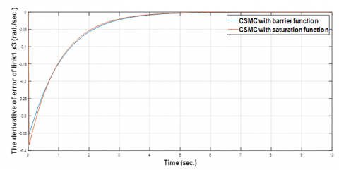
Figures 5 and 6 show the states' progression from their starting positions $x_1(0)=\frac{\pi}{8}, x_2(0)=\frac{\pi}{16}, x_3(0)=0$, and $x_4(0)=0$ for joint-1 and joint-2 till reaching equilibrium points (desired position) for CSMC with SF and with BF and as seen in Figures 7 and 8 the desired position. As a result, the system can be characterized as having global asymptotically stable because of convergence to the too-close neighborhood to zero (desired location) on the other means the error and the derivative of error are zero or near zero which leads to the exact tracking movement for the 2-link robot as seen in Figures 9-12.
Figure 5. The upward trajectory of calculated the SS uncertainty coefficients of joint-1 for CSMC with SF and BF
Figure 6. The upward trajectory of calculated the SS uncertainty coefficients of joint-2 for CSMC with SF and BF
Figure 7. The performance of tracking between both the actual and desired position of joint-1 for CSMC with SF and BF
Figure 8. The performance of tracking between both the actual and desired position of joint-2 for CSMC with SF and BF
Figure 9. The error of joint-1 (radians) for CSMC with SF and with BF
Figure 10. The error of joint-2 (radians) for CSMC with SF and with BF
Figure 11. The derivative of error of joint-1 (radians/seconds) for CSMC with SF and with BF
Figure 12. The derivative of error of joint-2 (radians/seconds) for CSMC with SF and with BF
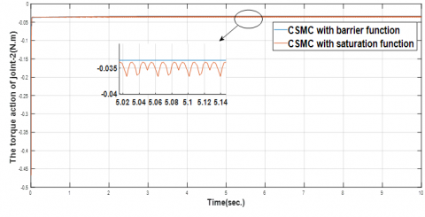
Figure 13 and Figure 14 displays the gain controller for each joint CSMC with SF and with BF, where it gives the high level which leads to optimizing the effort torque action, as seen in Figure 15 and Figure 16. When employing boundary layers (SF), the chatter persisted as seen in Figure 15 and Figure 16. In contrast, when using CSMC with BF, the chattering nearly completely disappeared.
Figure 13. The joint’s 1 classical gain k(x) of for CSMC with SF and with BF
Figure 14. The joint’s 2 classical gain k(x) for CSMC with SF and with BF
Figure 15. The joint’s 1 torque action (N.m.) for CSMC with SF and with BF
Figure 16. The joint’s 2 torque action (N.m.) for CSMC with SF and with BF
The data in Table 2 below illustrate the settling time and chattering intensity while administering the CSMC with SF and BF. It can be seen that the chattering decreased to a more tolerable level when using BF, and the settling time was shorter when using SF.
Table 2. Simulation results for CSMC
|
Content |
CSMC with Barrier Function |
CSMC with Saturation Function |
|
Settling time (sec.) |
4.5 |
4 |
|
The magnitude of chattering Beak to Beak (N. m.) |
≈0 |
1.00281 |
4.2 ASMC
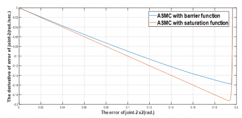
Figures 17 and 18 show the states' progression from their starting positions $x_1(0)=\frac{\pi}{8}, x_2(0)=\frac{\pi}{16}, x_3(0)=0$, and $x_4(0)=0$ for joint-1 and joint-2 till reaching equilibrium points (desired position) for CSMC with SF and with BF and as seen in Figures 19 and 20 the desired position. As a result, the system can be characterized as having global asymptotically stable because of convergence to the too-close neighborhood to zero (desired location) on the other means the error and the derivative of error are zero or near zero which leads to the exact tracking movement for the 2-link robot as seen in Figures 21-24.
Figure 17. The upward trajectory of calculated the SS uncertainty coefficients of joint-1 for ASMC with SF and BF
Figure 18. The upward trajectory of calculated the SS uncertainty coefficients of joint-2 for ASMC with SF and BF
Figure 19. The performance of tracking between both the actual and desired position of joint-1 for ASMC with SF and BF
Figure 20. The performance of tracking between both the actual and desired position of joint-2 for ASMC with SF and BF
Figure 21. The joint-1 error (radians) for ASMC with SF and with BFss
Figure 22. The joint-2 error (radians) for ASMC with SF and with BF
Figure 23. The derivative of error of joint-1 (radians/seconds) for ASMC with SF and with BF
Figure 24. The derivative of error of joint-2 (radians/seconds) for ASMC with SF and with BF
The controller’s gain of each joint for the ASMC with SF and with BF is illustrated in Figures 25 and 26. It provides a low level, which minimizes the effort torque action, as seen in Figures 27 and 28. When ASMC is used with BF, the chattering almost completely disappears, but when boundary layers (SF) are used, as in Figures 27 and 28, ASMC still exhibits chattering.
Figure 25. The joint’s 1 adaptive gain k(t) for ASMC with SF and with BF
Figure 26. The joint’s 2 adaptive gain k(t) for ASMC with SF and with BF
Figure 27. The joint’s 1 torque action (N.m.) for ASMC with SF and with BF
Figure 28. The joint’s 2 torque action (N.m.) for ASMC with SF and with BF
The information in Table 3 below illustrates the settling time and chattering intensity while applying the ASMC with SF and BF. It can be seen that chattering decreased to a more tolerable level while applying the ASMC with BF and that settling time is shorter when applying SF.
Table 3. Simulation results for ASMC
|
Content |
ASMC with Barrier Function |
ASMC with Saturation Function |
|
Settling time (sec.) |
4.5 |
4 |
|
The magnitude of chattering Beak to Beak (N. m.) |
0 |
0.012 |
In the presence of nonlinearity in the actuator, PU, CF, and ED, a robust SMC for a 2-link robot is constructed using the ASMC with BF concept. By lowering the controller gain to a more tolerable level, ASMC is used to improve the efficiency of CSMC. As a result, the control input is decreased. Unlike CSMC, ASMC doesn’t need the limit of uncertainty to be known, and the calculations of discontinued gain in cases when the limit of uncertainty is unknown would be affected by the motion of the 2-link robot and make it to follow the exact trajectory. Compared to SF, the simulation results in Figure 15, Figure 16 and Table 2 demonstrate that there will be no chattering when employing BF. Similar phenomena can be seen in ASMC in Figure 27, Figure 28 and Table 3 which led to the achievement of asymptotic stability. On the other hand, employing the SF in CSMC and ASMC results in a faster settling time than using the BF. However, BF ensures a zero chattering magnitude in contrast to SF, which has a tiny chattering magnitude; as a result, BF offers greater stability. On the other hand, even though it requires more settling time, BF is preferable to SF if accuracy is required for work. However, the SF will be a good option for the system if a shorter period is desired.
[1] Badoniya, P., George, J. (2018). Two link planar robot manipulator mechanism analysis with MATLAB. International Journal for Research in Applied Science & Engineering Technology, 6(7): 778-788. https://doi.org/10.22214/ijraset.2018.7132
[2] Baccouch, M., Dodds, S. (2020). A two-link robot manipulator: Simulation and control design. International Journal of Robotic Engineering, 5(2): 1-17. https://doi.org/10.35840/2631-5106/4128
[3] Elkhateeb, N., Badr, R.I. (2017). Novel PID tracking controller for 2DOF robotic manipulator system based on artificial bee colony algorithm. The Scientific Journal of Riga Technical University-Electrical, Control and Communication Engineering, 13: 55-62. https://doi.org/10.1515/ecce-2017-0008
[4] Jedda, O., Ghabi, J., Douik, A. (2017). Sliding mode control of an inverted pendulum. Applications of Sliding Mode Control, 105-118. https://doi.org/10.1007/978-981-10-2374-3_6
[5] Fulwani, D., Bandyopadhyay, B. (2013). Design of sliding mode controller with actuator saturation. In Advances in Sliding Mode Control: Concept, Theory and Implementation, pp. 207-219. https://doi.org/10.1007/978-3-642-36986-5_10
[6] Obeid, H., Fridman, L.M., Laghrouche, S., Harmouche, M. (2018). Barrier function-based adaptive sliding mode control. Automatica, 93: 540-544. https://doi.org/10.1016/j.automatica.2018.03.078
[7] Samanfar, A., Shakarami, M.R., Soltani Zamani, J., Rokrok, E. (2022). Adaptive sliding mode control for multi-machine power systems under normal and faulted conditions. Scientia Iranica, 29(5): 2526-2536. https://doi.org/10.24200/sci.2020.55717.4371
[8] Ajwad, S. A., Islam, R.U., Azam, M.R., Ullah, M.I., Iqbal, J. (2016). Sliding mode control of rigid-link anthropomorphic robotic arm. In 2016 2nd International Conference on Robotics and Artificial Intelligence (ICRAI), Rawalpindi, Pakistan, pp. 75-80. https://doi.org/10.1109/ICRAI.2016.7791232
[9] Armghan, A., Hassan, M., Armghan, H., Yang, M., Alenezi, F., Azeem, M.K., Ali, N. (2021). Barrier function based adaptive sliding mode controller for a hybrid AC/DC microgrid involving multiple renewables. Applied Sciences, 11(18): 8672. https://doi.org/10.3390/app11188672
[10] Tu'ma, D.H., Hamoudi, A.K. (2020). Performance of 2-link robot by utilizing adaptive sliding mode controller. Journal of Engineering, 26(12): 44-65. https://doi.org/10.31026/j.eng.2020.12.03
[11] Al-hadithy, D., Hammoudi, A. (2020). Two-link robot through strong and stable adaptive sliding mode controller. In 2020 13th International Conference on Developments in eSystems Engineering (DeSE), Liverpool, UK, pp. 121-127. https://doi.org/10.1109/DeSE51703.2020.9450762
[12] Shtessel, Y., Edwards, C., Fridman, L., Levant, A. (2014). Sliding mode control and observation. New York: Springer New York. https://doi.org/10.1007/978-0-8176-4893-0_8
[13] Hamoudi, A.K., Rahman, N.O.A. (2017). Design an integral sliding mode controller for a nonlinear system. Al-Khwarizmi Engineering Journal, 13(1): 138-147. https://doi.org/10.22153/kej.2017.09.003
[14] Tohma, D.H., Hamoudi, A.K. (2021). Design of adaptive sliding mode controller for uncertain pendulum system Engineering and Technology Journal, 39(3): 355-369. https://doi.org/10.30684/etj.v39i3A.1546
[15] Badri, S. (2014). Integral sliding mode controller design for electronic throttle valve. Doctoral dissertation, M. Sc. Thesis, Control and Systems Eng. Dept., Univ. of Technology, Baghdad, Iraq.
[16] Liu, J., Wang, X., Liu, J., Wang, X. (2011). Advanced Sliding Mode Control for Mechanical Systems: Design, Analysis and MATLAB Simulation, Springer Berlin, Heidelberg, pp. 117-135. https://doi.org/10.1007/978-3-642-20907-9_6
[17] Al-Samarraie, S.A., Midhat, B.F., Al-Deen, R.A.B. (2018). Adaptive sliding mode control for magnetic levitation system. Al-Nahrain Journal for Engineering Sciences, 21(2): 266-274. https://doi.org/10.29194/NJES21020266