Waleed Al-Ashtari*![]() | Karim H. Ali
| Karim H. Ali![]()
© 2023 IIETA. This article is published by IIETA and is licensed under the CC BY 4.0 license (http://creativecommons.org/licenses/by/4.0/).
OPEN ACCESS
This study presents a comprehensive exploration of the performance of a proposed controller within dynamic system contexts. The controller is rooted in Model Reference Adaptive Control (MRAC) and State Feedback Controller (SFC) techniques, offering a robust approach tailored specifically for Series Elastic Actuators (SEAs). This hybrid technique aims to overcome system uncertainties and attenuate load disturbances, thereby enhancing system performance and stability. Lyapunov stability analysis is employed to derive the adaptation mechanism, ensuring both the stability and efficacy of the controller. Additionally, the controller can be fine-tuned using a parameter, b. The study thoroughly analyzes the impact of this tuning parameter on suspension response. Through systematic simulations, an optimal value of is identified, and the controller's performance is investigated in terms of achieving the desired output with minimal settling time and control torque. At b = -80, the results demonstrate that the proposed controller efficiently achieves input tracking with a settling time of 1.95 seconds and a control torque reaching 7.39 Nm. The investigation extends to parameter uncertainties, highlighting the controller's adaptability to variations and showcasing its ability to proportionally adjust torque in response to parameter changes. Furthermore, the controller's resilience is validated under load disturbances, effectively demonstrating its capability to mitigate torque fluctuations and maintain desired angular positions. The results also indicate that the unit step disturbance causes a 49.9% increase in control torque, while the sinusoidal disturbance causes a 25% increase in control torque. Overall, this study underscores the controller's versatility, efficacy, and adaptive nature, positioning it as a valuable asset in the realm of SEA control applications.
MRAC, SFC, SEAs, Lyapunov stability analysis, and controller performance
The integration of a Series Elastic Actuator (SEA) represents a revolutionary advancement in the fields of robotics and mechatronics. By incorporating an elastic element in series with the motor, SEAs exhibit unparalleled attributes such as compliance, force sensing, and energy storage capabilities, surpassing the limitations of conventional rigid actuators. This distinctive design empowers the actuator to absorb, store, and judiciously release mechanical energy, enabling precise and adaptable movements.
The impetus behind SEAs lies in the pursuit of creating robotic systems that emulate human interaction and prioritize safety. By endowing robots with compliance through elastic elements, SEAs enhance responsiveness to external forces and dynamic environmental fluctuations, proving invaluable in physical engagement domains like collaborative robots (cobots), exoskeletons, prosthetics, rehabilitation devices, and diverse applications in healthcare and entertainment [1].
However, the adoption of SEAs introduces a set of complex challenges, including intricate design, energy inefficiency due to elastic effects, intricate control, and achieving stability, non-linear behavior, and demanding modeling. These intricacies necessitate innovative engineering solutions, novel control paradigms, and astute trade-off comprehension tailored to specific applications [2].
A hallmark feature of SEAs is their force-sensing ability, derived from the design's elasticity. The actuator, in real-time, discerns and quantifies external forces and torques. While this real-time force feedback proves invaluable in precision-critical applications, such as enabling robots to execute delicate tasks or adapt motions based on detected interactions, it also prompts the need for advanced control strategies [3].
In the realm of SEA control algorithms, two predominant categories are robust and adaptive controllers. Robust control aims to forge systems capable of withstanding uncertainties and disturbances without necessitating real-time adjustments, ensuring stability even in worst-case scenarios. In contrast, adaptive control continuously adapts settings based on real-time estimations of system dynamics, accommodating changes and minimizing disparities between desired and actual outputs [4].
Notably, these controllers, including PID Controllers, Sliding Mode Controllers (SMC), impedance controllers, SFC, MRAC, and Fuzzy Logic Controllers (FLC), may leverage either robust or adaptive control algorithms and may be used individually or combined to form hybrid controllers [5-10].
Within this context, a PID controller, widely utilized in diverse industries, calculates an output signal based on the discrepancy between the desired setpoint and the present process value, aiming for stable and precise process control. However, PID control may struggle with systems manifesting complex or highly nonlinear dynamics, compromising accuracy and stability [11-19].
SMC is a robust technique crafting a 'sliding surface' that mirrors a desired state trajectory, offering swift convergence and resilience to uncertainties. Yet, its susceptibility to high-frequency chattering requires consideration, potentially impacting stability and performance [20-30].
Impedance control, vital in robotics and mechatronics, regulates interactions between a robot and its environment by governing the dynamic interplay between applied forces or torques and ensuing displacements or velocities at the robot's end effector. While impedance control facilitates adaptable responses; discrepancies in system parameters or uncertainties can undermine its efficacy, impacting overall stability and performance [31-37].
State Feedback Control (SFC), governing dynamic systems based on internal state variables, finds application in diverse domains, achieving performance and stability by precise control. However, measurement errors or noise in accurate state measurements may compromise performance [38-47].
Model Reference Adaptive Control (MRAC), altering system control parameters in real-time to mirror a desired reference model, proves valuable in navigating systems with uncertain or time-varying dynamics. Yet, effective MRAC relies on accurate modeling of system dynamics, crucial for control performance [48-54].
FLC, mimicking human decision-making through linguistic variables and fuzzy sets, handles imprecise and uncertain data. FLC is advantageous in complex, nonlinear, or uncertain systems but requires expertise and iterative refinement [55-62].
The paper introduces an approach that integrates MRAC and SFC to effectively address challenges posed by SEAs. The anticipated benefit of this integration stems from the complementary strengths of MRAC and SFC. MRAC, known for its adaptability and robustness, compensates for uncertainties, while SFC, with its precision, contributes to accurate control based on internal state variables. This synergistic approach aims to enhance overall system performance, overcoming challenges such as intricate design, energy inefficiency, and control stability associated with SEAs. The combination leverages each approach's strengths to provide a comprehensive solution tailored to the specific challenges posed by SEAs. The hybrid technique is designed to overcome system uncertainties, reduce load disturbances, and improve the overall performance and stability of the system. Additionally, a lumped parameter model serves as the reference model, facilitating performance adjustment and the computation of necessary gains for the designed SFC. The calculation of an adaptation law, guided by Lyapunov's theory, incorporates terms aimed at enhancing system performance and mitigating parameter uncertainties and load disturbances.
As mentioned before, SEA is a type of actuator that incorporates an elastic element in series with the main actuation mechanism. The elastic element serves as a buffer between the actuator and the load it interacts with, providing several advantages for certain applications, particularly in areas where compliance and force control are essential. Figure 1 shows an illustrative diagram showing the equivalent lumped parameter model representing a SEA where a DC motor is selected to be the actuator mechanism. In Figure 1, the variables are defined as follows: u(t) represents the applied control torque, τ(t) denotes the disturbance torque arising from the load, θm(t) signifies the angular position of the motor side, and θl(t) denotes the angular position on the load side. Additionally, system parameters include Kb,Kj, and Bj, which respectively characterize the motor mounting stiffness, the elastic joint stiffness, and the elastic joint damping coefficient. Furthermore, Jm, and Jl represent the angular moment of inertia for the motor and the load, respectively.
Figure 1. Illustration of a SEA
Applying Newton’s second law of rotation to the motor side gives
Jm¨θm(t)+Bj(˙θm(t)−˙θl(t))+Kj(θm(t)−θl(t))+Kbθm(t)=u(t) (1)
Eq. (1) can be rewritten as
¨θm(t)=1Jm[−(Kj+Kb)θm(t)−Bj˙θm(t)+Kjθl(t)+Ki˙θl(t)+u(t)] (2)
Also, applying Newton’s second law of rotation to the load side gives
Jl¨θl(t)+Bj(˙θl(t)−˙θm(t))+Ki(θl(t)−θm(t))=−τ(t) (3)
Eq. (3) can be rearranged to be
¨θl(t)=1Jl[Kjθm(t)+Bj˙θm(t)−Kjθl(t)−Bj˙θl(t)−τ(t)] (4)
Assuming, x1(t)=θm(t),x2(t)=˙θm(t),x3(t)=θl(t), and x4(t)=˙θl(t), then substituting these into Eq. (2) and Eq. (4) gives
˙x2(t)=−(Kj+Kb)Jmx1(t)−BjJmx2(t)+KjJmx3(t)+BjJmx4(t)+1Jmu(t) (5)
and
˙x4(t)=KjJlx1(t)+BjJlx2(t)−KjJlx3(t)−BjJlx4(t)−1Jlτ(t) (6)
Now, rewriting Eq. (5) and Eq. (6) in the state space form
[˙x1(t)˙x2(t)˙x3(t)˙x4(t)]=[0100−(Kj+Kb)Jm−BjJmKjJmBjJm0001KjJlBjJl−KjJl−BjJl][x1(t)x2(t)x3(t)x4(t)]+[01Jm00]u(t)+[000−1Jl]τ(t) (7)
and the output state space
[y1(t)y2(t)y3(t)y4(t)]=[1000010000100001][x1(t)x2(t)x3(t)x4(t)] (8)
The system can then be represented by the following equation
˙x(t)=Ax(t)+Bu(t)+Wτ(t) (9)
and
y(t)=Cx(t) (10)
Here, x(t) denotes the system's state vector, and ˙x(t) is its derivative over time. The output vector of the system is represented by y(t). Additionally, A is the state matrix, B is the input matrix for applied torque, W is the input matrix for disturbance torque, and C is the output matrix. Upon comparing Eq. (7) and Eq. (9), notable observations emerge.
A=[0100−(Kj+Kb)Jm−BjJmKjJmBjJm0001KjJlBjJl−KjJl−BjJl] (11a)
B=[01Jm00]T (11b)
and
W=[000−1Jl]T (11c)
Also, the comparison between Eq. (8) and Eq. (10) gives
C=[1000010000100001] (11d)
The state matrix A governs the dynamic behavior of the system, influencing how it evolves over time. The input matrices B and W play crucial roles in controller design by determining how applied torque and disturbance torque, respectively, affect the system's response, while the output matrix C shapes the observed output of the controlled system.
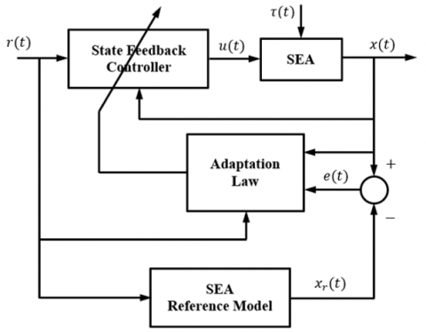
In the pursuit of optimizing the performance of a SEA, the implementation of a model reference approach stands out as a key technique. By utilizing this method, the detection of errors in the actuator's performance becomes more accurate and precise. To further enhance the actuator's capabilities, a controller grounded in state feedback theory is thoughtfully crafted. This controller, with its adept ability to calculate appropriate gains, effectively counters system uncertainties and disturbances while impeccably tracking the desired performance trajectory. One of the remarkable aspects of this design is the utilization of Lyapunov's theory, which serves as the guiding principle for continuously updating and adjusting the aforementioned gains. This process ensures a robust and adaptive actuation system that excels in meeting the ever-evolving challenges posed by real-world applications. Figure 2 shows the functional block diagram of the proposed controller.
Figure 2. Functional block diagram of the proposed controller
3.1 Reference model
Recalling Eq. (1) and Eq. (3) and rewriting them in simplifying them using the D-operator, i.e., D=d/dt, then the result is
θm(t)=1Jm[u(t)+(BjD+Kj)θl(t)D2+BjJmD+Kj+KbJm] (12)
and
θl(t)=−τ(t)+(BjD+Kj)θm(t)JlD2+BjD+Kj (13)
Assuming that both Eq. (12) and Eq. (13) have the standard form of the second-order system. This means that they can be rewritten as
θmr(t)=ω2n1u(t)D2+2ζ1ωn1D+ω2n1 (14)
θlr(t)=ω2n2θmr(t)D2+2ζ2ωn2D+ω2n2 (15)
where, θmr(t) and θlr(t) are the angular positions obtained by the reference model of the motor and load sides, respectively. Furthermore, the parameters ωn1,ωn2,ζ1, and ζ2 are the natural frequency of the motor side, the natural frequency of the load side, the damping ratio of the motor side, and the damping ratio of the load side, respectively. Again, if it is assumed that Assuming, xr1(t)=θmr(t),xr2(t)= ˙θmr(t),xr3(t)=θlr(t), and xr4(t)=˙θlr(t), the reference model can be expressed in the following state space form
˙xr(t)=Arxr(t)+Brr(t) (16)
and the output has this form
yr(t)=Crxr(t) (17)
then the system matrices of the reference model can be expressed as
Ar=[0100−ω2n1−2ζωn1000001ω2n20−ω2n2−2ζωn] (18a)
Br=[0ω2n100]T (18b)
and
Cr=C (18c)
where, xr(t) denotes the reference model state vector, and ˙xr(t) is its derivative over time. The output vector of the reference model is represented by yr(t). Additionally, Ar is the state matrix of the reference model, Br is the input matrix for the refence input r(t), and Cr is the output matrix of the reference model. In the current study, r(t) is a 1×4 column vector that serves as the representation of the desired reference input to be tracked.
A reference model serves as a guide for adjusting the performance of an actual system. This model represents the desired performance that the system should achieve. The designer customizes the performance of the reference model based on their preferences. The settling time of a system, ts, can be calculated using the Eq. (19):
ts=42ζωn (19)
To clarify, the goal is to have a settling time of 1 second for both sides of the system. Additionally, the damping ratios are set to 1 for both sides. This choice implies that the natural frequency ωn1 is equal to ωn2, and both are set to 4. In simpler terms, the reference model's settling time formula and parameter values are used to fine-tune the system's performance. Substituting these values in Eqs. (18a) and (18b) gives
Ar=[0100−16−8000001160−16−8] (20a)
and
Br=[01600]T (20b)
Eq. (16), Eq. (18c), Eq. (20a) and Eq. (20b) offer a comprehensive framework for characterizing the optimal response of SEAs.
3.2 Adaptive control law
The primary objective of the controller is to ensure that the behavior of the actual SEA follows the behavior of the reference model in order to achieve the desired outcome. Therefore, the error, e(t),can be expressed as
e(t)=x(t)−xr(t) (21)
Thus, the error rate of change, ˙e(t), can be written as
˙e(t)=˙x(t)−˙xr(t) (22)
Substituting Eq. (9) and Eq. (16) into Eq. (22) gives
˙e(t)=Ax(t)+Bu(t)−Arxr(t)−Brr(t) (23)
In this case, the disturbance torque is assumed to be zero, and the system takes on the conventional state space form. Expressing the control law can be achieved through the application of state feedback control theory, as illustrated below:
u(t)=krr(t)−kxx(t) (24)
where, kr and kx, are 1×4 vectors represent the gain of the reference input, and the feedback gain of the state. In fact, the integration of state feedback control theory with the reference model inherently addresses the impact of disturbances on the system. This integration compels the system to dynamically follow the reference input r(t), contingent upon the disparities between the states of the actual system and those of the reference model.
Substituting Eq. (23) into Eq. (24) results in the following expression:
˙e(t)=(A−Bkx)x(t)+(Bkr−Br)r(t)−Arxr(t) (25)
The controller's goal is to ensure that state x(t) tends to be identical to state xr(t), and hence the error is zero. This provides
Ar=A−Bkx (26)
and
Br=Bkr (27)
In real-life applications, the gains kx and kr cannot be calculated because the system parameters represented by the matrix A and B cannot be identified properly or they change over time due to friction, wear, deformation, etc. To overcome such a problem, the control law is reformulated to be
u(t)=ˆkr(t)r(t)−ˆkx(t)x(t) (28)
where, ˆkr(t) and ˆkx(t) are the estimations of kr and kx and have the same dimensions, respectively. Now, substituting Eq. (28) into Eq. (23), which gives
˙e(t)=(A−Bˆkx(t))x(t)+(Bˆkr(t)−Br)r(t)−Arxr(t) (29)
It can be noted that the estimation gains ˆkr(t) and ˆkx(t) are varying with time, and they can be expressed as
˜kr(t)=kr−ˆkr(t) (30a)
and
˜kx(t)=kx−ˆkx(t) (30b)
where, ˜kr(t) and ˜kx(t) are the estimation errors of kr and kx, respectively. Substituting Eqs. (30a) and (30b) into Eq. (29) gives
˙e(t)=(A−Bkx−B˜kx(t))x(t)+(Bkr−B˜kr(t)−Br)r(t)−Arxr(t) (31)
Further, substituting Eq. (26) and Eq. (27) into Eq. (31), which gives
˙e(t)=Are(t)−B˜kx(t)x(t)−B˜kr(t)r(t) (32)
Now, apply Lyapunov stability analysis to the following candidate function:
V(t)=12e2(t)+12˜k2r(t)+12˜k2x(t) (33)
The time derivative of the candidate function can be written as
˙V(t)=e(t)˙e(t)+˜kr(t)˜kr(t)+˜kx(t)˜kx(t) (34)
The time derivatives of ˜kr(t) and ˜kx(t) are
˙˜kx(t)=−˙ˆkx(t) (35a)
and
˙˜kr(t)=−˙ˆkr(t) (35b)
Substituting Eq. (35a), Eq. (35b), and Eq. (32) into Eq. (34), which leads to
˙V(t)=Are2(t)−Bx(t)e(t)˜kx(t)−Br(t)e(t)˜kr(t)−˙ˆkx(t)˜kx(t)−˙ˆkr(t)˜kr(t) (36)
In order to ensure that ˙V(t) goes to zero at time rans to infinity, then the following relationships should be provided
˙ˆkr(t)=−Br(t)e(t) (37a)
and
˙ˆkx(t)=−Bx(t)e(t) (37b)
As previously mentioned, since the system parameters are considered unknown, the vector B can be represented as follows:
B=b[0100]T (38)
Here, b is a constant utilized to fine-tune controller performance and tailor it based on the designer's preferences.
The proposed controller exhibits versatile applicability across SEAs and analogous systems. The incorporation of state feedback control integrated with a reference model establishes a flexible framework that can seamlessly adapt to diverse systems sharing similar dynamics. The fundamental principles and methodologies inherent in our model are inherently generalizable, streamlining the application process to different SEAs or systems that demonstrate akin characteristics. This inherent adaptability underscores the robustness and broad utility of our controller in addressing a spectrum of practical scenarios.
In this section, a comprehensive case study will be presented to rigorously validate the efficacy and performance of the proposed controller. The simulation model, crucial for this validation, has been meticulously crafted using MATLAB, a widely acknowledged platform for system modeling and analysis. This case study serves as a practical application of the proposed controller in a real-world context, shedding light on its capabilities and robustness.
Table 1. Parameters of simulated SEA
|
Physical Parameter |
Symbol |
Value |
Unit |
|
Motor side moment of inertia |
Jm |
0.1 |
kg m2 |
|
Load side moment of inertia |
Jl |
0.1 |
kg m2 |
|
Motor mounting stiffness |
Kb |
7 |
N/m |
|
Joint stiffness |
Kj |
3 |
N/m |
|
Joint damping coefficient |
Bj |
0.6 |
N s/m |
Table 1 provides the parameters employed in simulating the SEA in order to obtain the actual system response. Actually, the intention is to emulate a scenario where the parameters under consideration are deliberately assumed to be unknown. The purpose of this approach is to assess the controller's ability to generate a suitable response even in situations where vital parameters are not precisely known. This simulation-based investigation provides valuable insight into the controller's adaptability and robustness in real-world scenarios with uncertain or uncharacterized parameters. It is important to note that the utilization of these parameters solely for the purpose of eliciting responses adds an element of controlled unpredictability to the study, enabling a thorough evaluation of the proposed controller's performance under challenging and dynamic conditions.
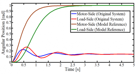
Figure 3 illustrates the dynamic behavior of angular positions over time, showcasing a comparison between the motor and load sides of both the reference model and the original SEA. The input applied to the system is a unit step. Evidently, the results highlight a significant disparity in performance. The original SEA system struggles to fulfill its intended task, with discernible deviations and oscillations in its response. In contrast, the reference model exhibits impeccable execution of the task, precisely tracking the desired angular positions. This marked divergence underscores the proficiency of the reference model-based controller in achieving superior control and response precision, even when compared to the inherent behavior of the original system.
Figure 3. Responses of the actual SEA and the reference model
Despite the similarity in the setup of both the motor and load sides within the reference model, an intriguing observation emerges from the results. It becomes evident that the desired 1s settling time is effectively achieved for the motor side, substantiating the model's capacity for rapid and precise response. However, it's noteworthy that such an optimized settling time is not attainable for the load side. This phenomenon can be attributed to the inherent dynamics and interplay within the reference model, where the motor side's output serves as the driving force for the load side.
Interestingly, despite this discrepancy in settling times between the two sides, the reference model remarkably upholds its promise of mimicking the ideal performance of the SEA. This underscores the model's proficiency in encapsulating the fundamental characteristics of the system and accurately replicating its behavior, even in cases where specific performance metrics might vary between components. The reference model's ability to consistently achieve the desired SEA performance substantiates its utility as a robust and effective control strategy, offering a valuable avenue for enhanced system performance and dynamic response.
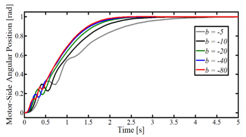
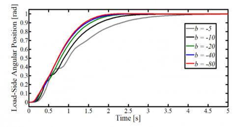
Various tuning gains for b have been methodically utilized to assess their influence on crucial aspects of the system. These include the angular positions of both the motor and load sides, along with the adaptively adjusted control torque. The selection of specific b values in our analysis resulted from an extensive series of simulations. The objective was to systematically investigate and illustrate the effects of diverse b values on the system's response and control torque. While the detailed exploration yields valuable insights into the variable's impact, the chosen values were deliberately tailored to present a comprehensive spectrum of scenarios, accentuating subtle nuances in the system's behavior across diverse conditions. The outcomes of these investigations are visually depicted in Figures 4, 5, and 6, respectively. As evident from Figures 4 and 5, the magnitude of b distinctly influences the velocity of the system's response. When b assumes a value of -5, the settling time, determined by the 2% criterion, extends to 3.46 seconds for both the motor and load sides. However, a substantial reduction in settling time is observed when b is set to -80, resulting in impressive durations of 1.95 seconds for the motor side and 1.81 seconds for the load side. Surprisingly, Figures 4 and 5 reveal that the system's response appears nearly indistinguishable at b values of -40 and -80. In contrast, Figure 6 emphasizes a subtle variance in control torque relative to the chosen b values, barring the instance of b at -80, which demonstrates a notable surge in control torque. Notably, Figure 6 also portrays the maximum control torque for b at -80, reaching 7.39 Nm, whereas for b at -40, the maximum control torque registers at 3.99 Nm. In light of these findings, the value of b equal to -40 is judiciously selected for further comprehensive investigation within this paper.
Figure 4. Response of the motor side of SEA
Figure 5. Response of the load side of SEA
Figure 6. Control torque variation
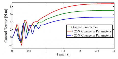
To comprehensively assess the controller's performance under scenarios where system parameters are either unknown or subject to change, an investigation has been undertaken. Specifically, a parameter variation of both +25% and -25% from the original values has been assumed. Remarkably, the results reveal a consistent pattern: the angular positions of both the motor and load sides remain unaltered in both cases, aligning precisely with the behaviors depicted in Figures 5 and 6, respectively. However, a significant variance is observed in the control torque, prominently displayed in Figure 7. At the point of steady-state operation, a distinct trend emerges: with a 25% increase in the parameters, the control torque experiences a corresponding 25% increase, effectively reflecting a proportional response to parameter fluctuations. Conversely, a 25% decrease in the parameters corresponds to a 25% reduction in the control torque. These findings underscore the controller's adaptive nature, where it adeptly compensates for parameter variations to maintain desired system behaviors, thus affirming its robustness and effectiveness within dynamic operational environments.
Figure 7. Control torque variation with parameters uncertainties
In order to thoroughly assess the efficacy of the proposed controller, a comprehensive evaluation across diverse operational conditions has been conducted. The analysis includes a meticulous study of the system's response to two distinct types of load disturbances: unit step and sinusoidal disturbances. It's important to note that there isn't a universally standardized form of disturbance applicable to most real-life scenarios. Hence, the deliberate choice of these two disturbance types aims to provide insights into the controller's performance under varied conditions. The sinusoidal disturbance introduced features a frequency of 1 Hz and an amplitude of 1 Nm. Notably, the angular positions of the system remain consistent for both types of disturbances, harmoniously aligning with those depicted in Figures 4 and 5 for the selected tuning gain of -40.
Intriguingly, Figure 8 effectively encapsulates the system's reaction to these disturbances. The unit step disturbance, when applied, triggers a substantial 49.4% surge in the control torque. This pronounced increase underscores the controller's capability to dynamically adapt and exert enhanced control authority in response to abrupt changes in the system. Equally noteworthy, the sinusoidal disturbance's effect on the control torque is comparatively milder, with a discernible 25.1% increase. This outcome reinforces the controller's adeptness in attenuating oscillatory influences, resulting in a more tempered response to periodic disturbances. This comprehensive assessment underscores the controller's versatile performance, adeptly addressing diverse disturbance scenarios and further establishing its efficacy in maintaining system stability and desired behaviors across varying operational contexts.
Figure 8. Control torque variation with disturbances
This paper highlights the revolutionary impact of SEAs in robotics and mechatronics, emphasizing their unique attributes such as compliance, force sensing, and energy storage. While SEAs address critical needs in human-robot interaction and safety, they also pose challenges like intricate design and control complexities. The paper proposes an innovative integration of MRAC and SFC to address SEA challenges. This hybrid approach aims to leverage the adaptability of MRAC and the precision of SFC, offering a comprehensive solution to enhance overall system performance and overcome challenges associated with SEAs, such as energy inefficiency and control stability. The use of a lumped parameter model and Lyapunov's theory guides the adaptation law, optimizing system performance and mitigating uncertainties and disturbances.
In conclusion, this study delves into a meticulous exploration of the performance and adaptability of the proposed controller within a dynamic system framework. The investigation encompasses various facets, each shedding light on the controller's robustness and efficacy. Through a systematic analysis of tuning gain b, the impact on the system's response was unveiled, revealing distinct settling times for varying b values. Notably, the reference model consistently demonstrated exceptional performance, even when settling times varied between the motor and load sides. This underscores the controller's potential to adeptly capture system behavior.
Moreover, the inquiry encompasses parameter uncertainties, deliberately chosen at a 25% variation in parameter values. These uncertainties were selected deliberately to be sufficiently substantial, allowing for a robust assessment of the controller's performance under challenging conditions. Impressively, despite parameter fluctuations, the angular positions remained consistent, reaffirming the controller's adaptability in maintaining desired behaviors. The proportional adjustment of control torque in response to parameter variations exemplified the controller's dynamic nature, robustly mitigating the effects of uncertain parameters. The results demonstrate that a 25% increase in parameters corresponds to a 25% increase in control torque, highlighting a proportional reaction to parameter changes. Conversely, a 25% reduction in parameters results in a corresponding 25% reduction in control torque.
The controller's prowess is further validated under load disturbances, showcasing its adaptability to external influences. Whether subjected to unit-step or sinusoidal disturbances, the controller exhibits commendable responses, adeptly mitigating surges in control torque and maintaining desired angular positions. These findings underscore the controller's versatility in managing diverse operational scenarios. Additionally, the results indicate that the application of a unit step disturbance leads to a 49.4% increase in control torque. This significant rise emphasizes the controller's ability to dynamically adapt and exercise expanded control authority in response to system changes. The effect of the sinusoidal disturbance on control torque is also notable, with a detectable 25.1% increase.
In summary, the proposed controller proves to be a robust and adaptive control strategy, effectively addressing uncertainties in parameters and dynamic disturbances. Its ability to uphold system stability, ensure precise control, and achieve desired behaviors across diverse challenges positions it as a valuable asset for optimizing system performance. Through a comprehensive exploration, this study underscores the controller's potential for real-world applications in dynamic systems, contributing to the evolution of control methodologies and enhancing operational outcomes. Looking ahead, future extensions of this study may involve implementing optimizing algorithms to determine the tuning parameter b. Additionally, consideration of non-linearities associated with SEAs could further broaden the scope of this research.
The authors would like to thank all the staff of the Mechanical Engineering Department, College of Engineering, University of Baghdad, for their support and assistance.
|
A |
state matrix |
|
Ar |
state matrix of the reference model |
|
B |
input matrix of the applied torque |
|
Bj |
elastic joint damping coefficient, N.m/(rad/s) |
|
Br |
input matrix for the refence input |
|
b |
fine-tuning parameter |
|
C |
output matrix |
|
Cr |
output matrix of the reference model |
|
e(t) |
error |
|
Jm |
motor side moment of inertia, kg m2 |
|
Jl |
load side moment of inertia, kg m2 |
|
Kb |
motor mounting stiffness, N.m/rad |
|
Kr |
gain vector of the refence input |
|
ˆkr(t) |
estimation of the gain kr |
|
˜kr(t) |
estimation error of the gain kr |
|
Kj |
elastic joint stiffness, N.m/rad |
|
Kx |
gain vector of the system state |
|
ˆkx(t) |
estimation of the gain kx |
|
˜kx(t) |
estimation error of the gain kx |
|
r(t) |
refence input |
|
ts |
settling time, s |
|
u(t) |
applied control torque, N.m |
|
V(t) |
candidate function of Lyapunov stability analysis |
|
W |
input matrix of the disturbance torque |
|
x(t) |
state variables of the system |
|
xr(t) |
state variables of the reference model |
|
y(t) |
output variables of system |
|
yr(t) |
output variables of reference model |
|
Greek symbols |
|
|
ζ |
damping ratio |
|
ζ1 |
damping ratio of the motor side |
|
ζ2 |
damping ratio of the load side |
|
θm(t) |
angular position of the motor side, rad/s |
|
θmr(t) |
angular position of the motor side of the reference model, rad/s |
|
θl(t) |
angular position of the load side, rad/s |
|
θlr(t) |
angular position of the load side of the reference model, rad/s |
|
τ(t) |
disturbance torque due to load N.m |
|
ωn |
natural frequency, rad/s |
|
ωn1 |
natural frequency of the motor side, rad/s |
|
ωn2 |
natural frequency of the load side, rad/s |
|
Subscripts |
|
|
FLC |
Fuzzy Logic Controller |
|
MRAC |
Model Refernce Adaptive Control |
|
PID |
Proportional-Integral-Derivative |
|
SEA |
Seies Elastic Actuator |
|
SFC |
State Feedback Controller |
|
SMC |
Sliding Mode Control |
[1] de Gea Fernández, J., Yu, B., Bargsten, V., Zipper, M., Sprengel, H. (2020). Design, modelling and control of novel series-elastic actuators for industrial robots. Actuators, 9(1): 6. https://doi.org/10.3390/act9010006
[2] Lee, C., Oh, S. (2019). Development, analysis, and control of series elastic actuator-driven robot leg. Frontiers in Neurorobotics, 13: 17. https://doi.org/10.3389/fnbot.2019.00017
[3] Cao, X., Aref, M.M., Mattila, J. (2019). Design and control of a flexible joint as a hydraulic series elastic actuator for manipulation applications. In 2019 IEEE International Conference on Cybernetics and Intelligent Systems (CIS) and IEEE Conference on Robotics, Automation and Mechatronics (RAM), Bangkok, Thailand, pp. 553-558. https://doi.org/10.1109/CIS-RAM47153.2019.9095773
[4] Calanca, A., Fiorini, P. (2014). Human-adaptive control of series elastic actuators. Robotica, 32(8): 1301-1316. https://doi.org/10.1017/S0263574714001519
[5] Shao, N., Zhou, Q., Shao, C., Zhao, Y. (2021). Adaptive control of robot series elastic drive joint based on optimized radial basis function neural network. International Journal of Social Robotics, 13(7): 1823-1832. https://doi.org/10.1007/s12369-021-00762-0
[6] Nguyen, M.N., Tran, D.T., Ahn, K.K. (2018). Robust position and vibration control of an electrohydraulic series elastic manipulator against disturbance generated by a variable stiffness actuator. Mechatronics, 52: 22-35. https://doi.org/10.1016/j.mechatronics.2018.04.004
[7] Wei, Y., Wang, H., Tian, Y. (2023). Adaptive time-varying barrier Lyapunov function-based model-free hybrid position/force control for series elastic actuator-based manipulator. IEEE Transactions on Circuits and Systems II: Express Briefs. https://doi.org/10.1109/TCSII.2023.3297600
[8] Kordik, T., Gattringer, H., Müller, A. (2023). Hybrid position‐compliance control of redundantly actuated parallel kinematic manipulators equipped with serial elastic actuators. Proceedings in Applied Mathematics & Mechanics, 22(1): e202200195. https://doi.org/10.1002/pamm.202200195
[9] Sariyildiz, E. (2022). A unified robust motion controller synthesis for compliant robots driven by series elastic actuators. In 2022 IEEE 17th International Conference on Advanced Motion Control (AMC), Padova, Italy, pp. 402-407. https://doi.org/10.1109/AMC51637.2022.9729316
[10] Bolívar, E., Rezazadeh, S., Summers, T., Gregg, R.D. (2019). Robust optimal design of energy efficient series elastic actuators: Application to a powered prosthetic ankle. In 2019 IEEE 16th International Conference on Rehabilitation Robotics (ICORR), Toronto, ON, Canada, pp. 740-747. https://doi.org/10.1109/ICORR.2019.8779446
[11] Norouzi, G.S., Akbarzadeh, A.R. (2015). Prismatic series elastic actuator: Modelling and control by ICA and PSO-tuned fractional order PID. International Journal of Advanced Design & Manufacturing Technology, 8(4): 23-32.
[12] Copot, C., Muresan, C., MacThi, T., Ionescu, C. (2018). An application to robot manipulator joint control by using constrained PID based PSO. In 2018 IEEE 12th International Symposium on Applied Computational Intelligence and Informatics (SACI), Timisoara, Romania, pp. 000279-000284. https://doi.org/10.1109/SACI.2018.8440927
[13] Bingol, M.C., Akpolat, Z.H., Koca, G.O. (2018). Robust control of a robot arm using an optimized PID controller. In Mechatronics 2017: Recent Technological and Scientific Advances, Gliwice, Poland, pp. 484-492. https://doi.org/10.1007/978-3-319-65960-2_60
[14] Naing, W.W., Thanlyin, M., Aung, K.Z., Thike, A. (2018). Position control of 3-DOF articulated robot arm using PID controller. International Journal of Science and Engineering Applications, 7(9): 254-260.
[15] Ghidini, S., Beschi, M., Pedrocchi, N., Visioli, A. (2018). Robust tuning rules for series elastic actuator PID cascade controllers. IFAC-PapersOnLine, 51(4): 220-225. https://doi.org/10.1016/j.ifacol.2018.06.069
[16] Ahmad, M.A., Ishak, H., Nasir, A.N.K., Abd Ghani, N. (2021). Data-based PID control of flexible joint robot using adaptive safe experimentation dynamics algorithm. Bulletin of Electrical Engineering and Informatics, 10(1): 79-85. https://doi.org/10.11591/eei.v10i1.2472
[17] Rohman, M., Saputra, D.I. (2021). Modeling and controlling the actuator joint angle position on the robot arm base using discrete PID algorithm. Ultima Computing: Jurnal Sistem Komputer, 13(2): 50-56. https://doi.org/10.31937/sk.v13i2.2103
[18] Batiha, I.M., Njadat, S.A., Batyha, R.M., Zraiqat, A., Dababneh, A., Momani, S. (2022). Design fractional-order PID controllers for single-joint robot arm model. International Journal of Advances in Soft Computing and its Applications, 14(2): 96-114. https://doi.org/10.15849/IJASCA.220720.07
[19] Sersar, A., Debbat, M.B. (2022). Series elastic actuator cascade PID controller design using genetic algorithm method. In International Conference on Artificial Intelligence: Theories and Applications, Mascara, Algeria, pp. 202-211. https://doi.org/10.1007/978-3-031-28540-0_16
[20] Yin, W., Sun, L., Wang, M., Liu, J. (2018). Robust position control of series elastic actuator with sliding mode like and disturbance observer. In 2018 Annual American Control Conference (ACC), Milwaukee, WI, USA, pp. 4221-4226. https://doi.org/10.23919/ACC.2018.8431653
[21] Soltanpour, M.R., Moattari, M. (2019). Voltage based sliding mode control of flexible joint robot manipulators in presence of uncertainties. Robotics and Autonomous Systems, 118: 204-219. https://doi.org/10.1016/j.robot.2019.05.014
[22] Rsetam, K., Cao, Z., Man, Z. (2019). Cascaded-extended-state-observer-based sliding-mode control for underactuated flexible joint robot. IEEE Transactions on Industrial Electronics, 67(12): 10822-10832. https://doi.org/10.1109/TIE.2019.2958283
[23] Gong, X., Sun, L., Liu, J. (2019). Proxy based sliding mode control for series elastic actuator based on algebraic identification and motion planning. Chinese Control and Decision Conference (CCDC), Nanchang, China, pp. 863-868. https://doi.org/10.1109/CCDC.2019.8832935
[24] Azar, A.T., Serrano, F.E., Koubâa, A., Kamal, N.A., Vaidyanathan, S., Fekik, A. (2019). Adaptive terminal-integral sliding mode force control of elastic joint robot manipulators in the presence of hysteresis. In International Conference on Advanced Intelligent Systems and Informatics, Cairo, Egypt, pp. 266-276. https://doi.org/10.1007/978-3-030-31129-2_25
[25] Sun, H.J., Ye, J., Chen, G. (2021). Trajectory tracking of series elastic actuators using terminal sliding mode control. In 2021 33rd Chinese Control and Decision Conference (CCDC), Kunming, China, pp. 189-194. https://doi.org/10.1109/CCDC52312.2021.9601778
[26] Cheng, X., Liu, H., Lu, W. (2021). Chattering-suppressed sliding mode control for flexible-joint robot manipulators. Actuators, 10(11): 288. https://doi.org/10.3390/act10110288
[27] Rsetam, K., Cao, Z., Man, Z. (2021). Design of robust terminal sliding mode control for underactuated flexible joint robot. IEEE Transactions on Systems, Man, and Cybernetics: Systems, 52(7): 4272-4285. https://doi.org/10.1109/TSMC.2021.3096835
[28] Wang, H., Zhang, Z., Tang, X., Zhao, Z., Yan, Y. (2022). Continuous output feedback sliding mode control for underactuated flexible-joint robot. Journal of the Franklin Institute, 359(15): 7847-7865. https://doi.org/10.1016/j.jfranklin.2022.08.020
[29] Yokoyama, M., Shimono, T., Uzunović, T., Šabanović, A. (2023). Sliding mode-based design of unified force and position control for series elastic actuator. In 2023 IEEE International Conference on Mechatronics (ICM), Loughborough, UK, pp. 1-6. https://doi.org/10.1109/ICM54990.2023.10101901
[30] Guo, Z., Wei, Y. (2023). Disturbance observer-based sliding mode control of series elastic actuators with unmatched disturbances. Discrete and Continuous Dynamical Systems-S, 16(7): 1964-1979. https://doi.org/10.3934/dcdss.2023094
[31] Haninger, K., Asignacion, A., Oh, S. (2019). Safe rendering of high impedance on a series-elastic actuator with disturbance observer-based torque control. arXiv preprint arXiv:1912.01355. https://doi.org/10.48550/arXiv.1912.01355
[32] Lee, C., Cheon, D., Oh, S. (2019). High fidelity impedance control of series elastic actuator for physical human-machine interaction. In IECON 2019-45th Annual Conference of the IEEE Industrial Electronics Society, Lisbon, Portugal, pp. 3621-3626. https://doi.org/10.1109/IECON.2019.8927520
[33] Mustalahti, P., Mattila, J. (2020). Impedance control of hydraulic series elastic actuator with a model-based control design. In 2020 IEEE/ASME International Conference on Advanced Intelligent Mechatronics (AIM), Boston, MA, USA, pp. 966-971. https://doi.org/10.1109/AIM43001.2020.9158817
[34] Haninger, K., Asignacion, A., Oh, S. (2020). Safe high impedance control of a series-elastic actuator with a disturbance observer. In 2020 IEEE International Conference on Robotics and Automation (ICRA), Paris, France, pp. 921-927. https://doi.org/10.1109/ICRA40945.2020.9197402
[35] Fotuhi, M.J., Bingul, Z. (2021). Novel fractional hybrid impedance control of series elastic muscle-tendon actuator. Industrial Robot: The International Journal of Robotics Research and Application, 48(4): 532-543. https://doi.org/10.1108/IR-10-2020-0236
[36] Mustalahti, P., Mattila, J. (2022). Position-based impedance control design for a hydraulically actuated series elastic actuator. Energies, 15(7): 2503. https://doi.org/10.3390/en15072503
[37] Gu, J., Xu, C., Liu, K., Zhao, L., He, T., Sun, Z. (2022). Impedance control of upper limb rehabilitation robot based on series elastic actuator. In International Conference on Intelligent Robotics and Applications, Harbin, China, pp. 138-149. https://doi.org/10.1007/978-3-031-13835-5_13
[38] Liu, H., Huang, Y. (2018). Robust adaptive output feedback tracking control for flexible-joint robot manipulators based on singularly perturbed decoupling. Robotica, 36(6): 822-838. https://doi.org/10.1017/S0263574718000061
[39] Zeng, Z., Cheng, X., Liu, H. (2018). Saturated output feedback control for flexible-joint robot manipulators. In 2018 Chinese Automation Congress (CAC), Xi'an, China, pp. 2194-2200. https://doi.org/10.1109/CAC.2018.8623387
[40] Yin, W., Sun, L., Wang, M., Liu, J. (2018). Nonlinear state feedback position control for flexible joint robot with energy shaping. Robotics and Autonomous Systems, 99: 121-134. https://doi.org/10.1016/j.robot.2017.10.007
[41] Calanca, A., Fiorini, P. (2018). A rationale for acceleration feedback in force control of series elastic actuators. IEEE Transactions on Robotics, 34(1): 48-61. https://doi.org/10.1109/TRO.2017.2765667
[42] Hua, T.M., Sanfilippo, F., Helgerud, E. (2019). A robust two-feedback loops position control algorithm for compliant low-cost series elastic actuators. In 2019 IEEE International Conference on Systems, Man and Cybernetics (SMC), Bari, Italy, pp. 2384-2390. https://doi.org/10.1109/SMC.2019.8913845
[43] Jia, P. (2019). Control of flexible joint robot based on motor state feedback and dynamic surface approach. Journal of Control Science and Engineering, 2019: 5431636. https://doi.org/10.1155/2019/5431636
[44] Shardyko, I., Samorodova, M., Titov, V. (2021). Series elastic actuator control based on active damping injection with positive torque feedback. In 2021 International Conference on Industrial Engineering, Applications and Manufacturing (ICIEAM), Sochi, Russia, pp. 613-618. https://doi.org/10.1109/ICIEAM51226.2021.9446352
[45] Zha, T., Li, P., Xu, Y., Gong, X., Sun, L. (2021). Saturation functions based control for series elastic actuator with feedback linearization. In 2021 40th Chinese Control Conference (CCC), Shanghai, China, pp. 253-259. https://doi.org/10.23919/CCC52363.2021.9550514
[46] Wang, J., Zhang, H., Dong, H., Zhao, J. (2021). Partial-state feedback based dynamic surface motion control for series elastic actuators. Mechanical Systems and Signal Processing, 160: 107837. https://doi.org/10.1016/j.ymssp.2021.107837
[47] Spyrakos-Papastavridis, E., Fu, Z., Dai, J.S. (2022). Power-shaping model-based control with feedback deactivation for flexible-joint robot interaction. IEEE Robotics and Automation Letters, 7(2): 4566-4573. https://doi.org/10.1109/LRA.2022.3144781
[48] Ghidini, S., Beschi, M., Pedrocchi, N. (2020). A robust linear control strategy to enhance damping of a series elastic actuator on a collaborative robot. Journal of Intelligent & Robotic Systems, 98: 627-641. https://doi.org/10.1007/s10846-019-01071-5
[49] Tran, M. S., Jung, S.H., Le, N.B., Nguyen, H.H., Dang, D.C., Tran, A.M.D., Kim, Y.B. (2020). Model reference adaptive control strategy for application to robot manipulators. In AETA 2018-Recent Advances in Electrical Engineering and Related Sciences: Theory and Application, Ostrava, Czech Republic, pp. 533-547. https://doi.org/10.1007/978-3-030-14907-9_53
[50] Sanfilippo, F., Hua, T.M., Bos, S. (2020). A comparison between a two feedback control loop and a reinforcement learning algorithm for compliant low-cost series elastic actuators. In Proceeding of the 53rd Hawaii International Conference on System Sciences (HICSS 2020), pp. 881-890.
[51] Tuan, H.M., Sanfilippo, F., Hao, N.V. (2021). Modelling and control of a 2-DOF robot arm with elastic joints for safe human-robot interaction. Frontiers in Robotics and AI, 8: 679304. https://doi.org/10.3389/frobt.2021.679304
[52] Tuan, H.M., Sanfilippo, F., Hao, N.V. (2022). A novel adaptive sliding mode controller for a 2-DOF elastic robotic arm. Robotics, 11(2): 47. https://doi.org/10.3390/robotics11020047
[53] Lanh, L.A.K., Duong, V.T., Nguyen, H.H., Kim, S.B., Nguyen, T.T. (2023). Hybrid adaptive control for series elastic actuator of humanoid robot. International Journal of Intelligent Unmanned Systems, 11(3): 359-377. https://doi.org/10.1108/IJIUS-07-2021-0071
[54] Rampeltshammer, W., Keemink, A., Sytsma, M., van Asseldonk, E., van der Kooij, H. (2023). Evaluation and comparison of SEA torque controllers in a unified framework. Actuators, 12(8): 303. https://doi.org/10.3390/act12080303
[55] Ling, S., Wang, H., Liu, P.X. (2019). Adaptive fuzzy dynamic surface control of flexible-joint robot systems with input saturation. IEEE/CAA Journal of Automatica Sinica, 6(1): 97-107. https://doi.org/10.1109/JAS.2019.1911330
[56] Tavoosi, J., Mohammadi, F. (2019). A new type-II fuzzy system for flexible-joint robot arm control. In 2019 6th International Conference on Control, Instrumentation and Automation (ICCIA), Sanandaj, Iran, pp. 1-4. https://doi.org/10.1109/ICCIA49288.2019.9030872
[57] Loraki, A.R., Ashourian, M. (2019). Adaptive neural fuzzy observer design for flexible robot joint control. Majlesi Journal of Mechatronic Systems, 8(2): 39-54.
[58] Song, B., Lee, D., Park, S.Y., Baek, Y S. (2020). A novel method for designing motion profiles based on a fuzzy logic algorithm using the hip joint angles of a lower-limb exoskeleton robot. Applied Sciences, 10(19): 6852. https://doi.org/10.3390/app10196852
[59] Zaare, S., Soltanpour, M.R. (2022). Adaptive fuzzy global coupled nonsingular fast terminal sliding mode control of n-rigid-link elastic-joint robot manipulators in presence of uncertainties. Mechanical Systems and Signal Processing, 163: 108165. https://doi.org/10.1016/j.ymssp.2021.108165
[60] Souzanchi-K, M., Akbarzadeh-T, M.R., Naghavi, N., Sharifnezhad, A., Khoshdel, V. (2022). Adaptive fuzzy robust tracking control using human electromyogram signals for elastic joint robots. Intelligent Automation & Soft Computing, 34(1): 279-294. http://dx.doi.org/10.32604/iasc.2022.023717
[61] Shao, J., Bian, Y., Yang, M., Liu, G. (2022). High precision adaptive fuzzy control method for hydraulic robot joint. In 2022 IEEE 13th International Conference on Mechanical and Intelligent Manufacturing Technologies (ICMIMT), Cape Town, South Africa, pp. 285-290. https://doi.org/10.1109/ICMIMT55556.2022.9845247
[62] Elouni, M., Hamdi, H., Rabaoui, B., BenHadj Braiek, N. (2022). Adaptive PID fault-tolerant tracking controller for Takagi-Sugeno fuzzy systems with actuator faults: Application to single-link flexible joint robot. International Journal of Robotics & Control Systems, 2(3): 523-546. https://doi.org/10.31763/ijrcs.v2i3.762