Robust H∞ Optimal Control for Longitudinal and Lateral Dynamics in Small-Scale Helicopters

Kared Saber*![]() | Mechhoud Elarkam
| Mechhoud Elarkam![]() | Ahmida Zahir
| Ahmida Zahir![]() | Mohand Said Larabi
| Mohand Said Larabi![]() | Ilhami Colak
| Ilhami Colak![]()
© 2023 IIETA. This article is published by IIETA and is licensed under the CC BY 4.0 license (http://creativecommons.org/licenses/by/4.0/).
OPEN ACCESS
In the field of unmanned aerial vehicle control, the pursuit of robustness and optimality in the presence of uncertainties and disturbances remains a paramount challenge, particularly for small-scale helicopters. This study addresses the robust optimal control of longitudinal and lateral flight dynamics using the mixed sensitivity H∞ norm approach. The focus lies on achieving a control system that not only stabilizes but also excels in performance under various flight conditions, including hovering and translational maneuvers. The adopted methodology commences with the derivation of a mathematical model reflecting the system dynamics, characterized by six degrees of freedom and nonlinearities with inherent unstable coupling dynamics. Subsequent linearization of this model employs a Taylor approximation near an operational point, effectively transforming the complex nonlinear system into a more tractable linear form. To incorporate real-world applicability, this model is augmented with representations of uncertainties and external disturbances, acknowledging the unpredictable nature of aerial environments. The crux of this research lies in the implementation of the mixed sensitivity design method for H∞feedback control. This approach is meticulously applied to the longitudinal and lateral motion subsystems, with a critical emphasis on maintaining system robustness in the face of the aforementioned uncertainties and disturbances. The evaluation of the controller's efficacy is based on qualitative performance metrics, such as response speed and overshoot characteristics. Simulation results demonstrate that the designed controller adeptly manages the intricate multi-input multi-output system, maintaining commendable control performance even under deterministic disturbances and noise. These findings contribute significantly to the unmanned aerial vehicle field, offering a robust control solution for small-scale helicopters that navigate complex environments. The methodology and results presented here hold promise for broader applications in unmanned aerial systems, where stability and adaptability in uncertain conditions are crucial.
unmanned small-scale helicopter, longitudinal-lateral flight, mixed sensitivity, disturbance, uncertainties, H∞
Recent advancements in drone technology have garnered significant attention in both civil and military sectors, owing to their multifaceted applications in security, agriculture, and emergency response. Among various drone types, unmanned small-scale helicopters have emerged as a subject of considerable interest. These helicopters are distinguished by their complex aerodynamic model, characterized by nonlinear dynamics and a six-degree-of-freedom actuation system. This introduction reviews pertinent research in the fields of modeling and control of these systems, highlighting key contributions and identifying gaps in the current state of knowledge.
The mathematical modeling of small-scale helicopter dynamics has been a focal point of research. Gavrilets et al. [1] presented a seminal work on the dynamic modeling of miniature helicopters, specifically a model developed for NAZA's 'Minimum-Complexity Helicopter Simulation Math Model'. This model's linearization, utilizing Taylor expansion approximation at various equilibrium points, was further elaborated by Yechout et al. [2]. Concurrently, advancements in control techniques for these helicopters have been noteworthy. Wang et al. [3] designed a robust controller improving roll and pitch attitude control across varying flight amplitudes. Comparative studies of robust control techniques, such as ADRC and DOBC, for disturbance estimation in small-scale helicopters have been investigated by Yu et al. [4].
Moreover, integrated approaches for identification and control of these systems were explored by Ma et al. [5], while Choudhary [6] focused on the H∞ optimal feedback control of a twin rotor MIMO system, demonstrating effective cross-coupling management. However, the evaluation of weight functions for controller robustness in Choudhary's study warrants further investigation, particularly in disturbance rejection and noise measurement. This study aims to extend these tests, simulating various disturbance and noise scenarios to enhance controller robustness and stability.
Other notable contributions include the work of Khalesi et al. [7], who explored the dynamics and control of roll and pitch in unmanned marine vehicles (UMVs), although their results indicated discrepancies in tracking the vertical Euler angle. Sahin and Kasnakoğlu [8] concentrated on linearizing UMVs around equilibrium points and stabilizing them through local controllers. Yan et al. [9] developed an adaptive robust fault-tolerant control for attitude tracking in helicopters, effectively managing actuator faults and external disturbances.
In the research led by Duan et al. [10], a quaternion-based adaptive dynamic surface control method is proposed, specifically designed for the attitude tracking of small-scale unmanned helicopters, addressing external disturbances and uncertain dynamics. Said et al. [11] explored the robustness of a controller based on the mixed sensitivity approach, focusing on trajectory tracking of a multivariable quad-rotor drone amidst disturbances, and benchmarking it against a PID controller. Papalambrou et al. [12] concentrated on the selection of optimal weighting functions for robust control, quantifying uncertainties and disturbances in line with the robustness conditions set by Doyle and Stein [13]. This study aims to extend these methodologies, particularly in refining the choice of weighting functions to enhance controller performance under variable conditions.
This study addresses a gap in the current literature, which predominantly focuses on the hovering maneuver of small-scale helicopters, a simplification that does not fully encapsulate the complexities of their operational dynamics. This research expands the scope to include both hovering and forward translation flights, taking into account output disturbances, noise, and parameter uncertainties. The central contribution of this work is the development of an optimal robust controller, specifically engineered to ensure precise tracking performance under these varied conditions. This controller is designed to integrate the full state vector, enabling comprehensive tracking of all state variables within the state space.
The structure of the paper is methodically organized into five distinct sections. The first section delves into the mathematical modeling of the UMV, laying the foundational framework for the study. The second section is dedicated to describing the $\mathrm{H}_{\infty}$ optimal feedback control algorithm, a critical component of the research. Following this, the third section applies the $\mathrm{H}_{\infty}$ optimal feedback controller to the helicopter, demonstrating its practical implementation. The fourth section presents the results and engages in a detailed discussion of the findings. Finally, the paper concludes with a summary of the research, its implications, and potential avenues for future study.
2.1 System modeling of small-scale unmanned helicopter (SSUH)
The SSUH represents an advanced flying machine, capable of autonomous or semi-autonomous operations. It is increasingly utilized in both military and civilian contexts for tasks such as supervision and reconnaissance, offering safe and efficient mission execution. The SSUH is characterized as a multi-input/multi-output (MIMO) system with six degrees of freedom, exhibiting significant nonlinearity and coupling effects.
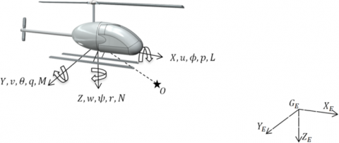
To accurately model the SSUH, it is essential to formulate both translation and rotation equations, treating the helicopter as a rigid body. The system's dynamics are defined by time-varying velocity components (u, v, w) and angular velocities (p, q, r), driven by applied forces (X, Y, Z) and moments (L, M, N), as depicted in Fig. 1. These axes undergo changes in response to the forces and moments acting on the helicopter.
For the development of a dynamic model, two reference frames are indispensable: the Earth frame $E\left[G_E, X_E, Y_E, Z_E\right]$, which serves as a stationary reference, and the body frame $B\left[G_B, X_B, Y_B Z_B\right]$, centered at the helicopter's gravity center $G$. The equations are constructed by considering an arbitrary material point $O$ in these frames, including the inertial frame (I).
In the course of the helicopter's motion, all variables are expressed in the body frame (B).
The computation of the absolute acceleration of a material point $O$ involves summing the acceleration of Orelative to $G_B$ and its acceleration relative to the fixed Earth frame $E\left[G_E, X_E, Y_E, Z_E\right]$. This modeling process starts by examining the position vector of point $O$ relative to $G_B$, thereby establishing a comprehensive and precise model of the helicopter's dynamics.
Figure 1. Coordinates of helicopter
In the phase of motion analysis, it is crucial to understand the transformation of vectors or points between different reference frames, as highlighted by Ding et al. [14]. This study utilizes Euler angles (Eq. (1)), as illustrated in Figure 1, to facilitate these transformations between the Earth and body frames.
$R=\left[\begin{array}{ccc}\mathrm{C}_\theta \mathrm{C}_\psi & \mathrm{C}_\psi \mathrm{S}_\phi \mathrm{S}_\theta-\mathrm{C}_\phi \mathrm{S}_\psi & \mathrm{S}_\phi \mathrm{S}_\psi+\mathrm{C}_\phi \mathrm{C}_\psi \mathrm{S}_\theta \\ \mathrm{C}_\theta \mathrm{S}_\psi & \mathrm{C}_\phi \mathrm{C}_\psi+\mathrm{S}_\phi \mathrm{S}_\theta \mathrm{S}_\psi & \mathrm{C}_\phi \mathrm{S}_\theta \mathrm{S}_\psi-\mathrm{C}_\psi \mathrm{S}_\phi \\ -\mathrm{S}_\theta & \mathrm{C}_\theta \mathrm{S}_\phi & \mathrm{C}_\phi \mathrm{C}_\theta\end{array}\right]$ (1)
where, $\mathrm{C}_\theta=\cos (\theta), \mathrm{S}_\theta=\sin (\theta)$
Considering the system's six degrees of freedom, several simplifying assumptions are made to model the helicopter dynamics effectively:
•Solid Body Approximation: The helicopter is treated as a rigid, solid body.
•Neglect of Aerodynamic Forces: Aerodynamic forces, which can be complex and difficult to model accurately, are neglected in this analysis.
•Small Angle Approximations: The model employs small angle approximations, which assume that the Euler angles are sufficiently small so that their higher-order terms can be ignored.
These assumptions are reasonable and common in the study of small-scale helicopters. Due to the reduced dimensions of these helicopters, such simplifications allow for a sufficiently accurate description of their dynamics. Particularly, the rigid body assumption is a standard practice in this research area. Moreover, the impact of airflow induced by the main rotor on the helicopter's fuselage is considered negligible compared to the forces produced by the main and tail rotors, further supporting the validity of these assumptions.
2.1.1 SSUH mechanics and kinematics equations
To construct the nonlinear model of the SSUH, it is essential to formulate the equations for forces, moments, and kinematics in accordance with Newton's second law, as outlined by Venkatesan [15]. These equations form the basis for understanding the helicopter's dynamics.
•Force equations
$\left\{\begin{array}{l}\dot{U}=R V-Q W-g \sin \theta+\frac{X_u}{m} \\ \dot{V}=P W-R U+g \sin \phi \cos \theta+\frac{Y_v}{m} \\ \dot{W}=Q U-P V+g \cos \phi \cos \theta+\frac{Z_w}{m}\end{array}\right.$ (2)
•Moment equations
$\left\{\begin{array}{l}\dot{Q}=\frac{P R\left(I_{Z Z}-I_{X X}\right)}{I_{Y Y}}+\frac{M}{I_{Y Y}}-\frac{\left(P^2-R^2\right)}{I_{Y Y}} I_{X Z} \\ \dot{P}=-\frac{Q R\left(I_{Z Z}-I_{Y Y}\right)}{I_{X X}}+\frac{(\dot{R}-P Q)}{I_{X X}} I_{X Z}+\frac{L}{I_{X X}} \\ \dot{R}=-\frac{P Q\left(I_{Y Y}-I_{X X}\right)}{I_{Z Z}}-\frac{(Q R-\dot{P})}{I_{Z Z}} I_{X Z}+\frac{N}{I_{Z Z}}\end{array}\right.$ (3)
In order to streamline the study of the helicopter's characteristics, a simplified mathematical model is adopted. The helicopter's hovering position, where all linear and angular velocities are zero, is chosen as the equilibrium point. Around this point, the nonlinear model of the helicopter is linearized using the Taylor approximation technique, a method detailed by the studies [16, 17].
Each motion variable – including forces, moments, and Euler angles – is redefined as the sum of a steady-state value and a disturbance value.
$\begin{aligned} & \left\{\begin{array}{l}V=V_0+v \\ U=U_0+u\end{array}\left\{\begin{array}{c}\Theta=\Theta_0+\theta \\ \Phi=\Phi_0+\phi\end{array}\right.\right. \\ & \left\{\begin{array}{l}\mathrm{P}=\mathrm{P}_0+p \\ \mathrm{Q}=\mathrm{Q}_0+q\end{array}\left\{\begin{array}{c}W=W_0+w \\ R=R_0+r\end{array}\right.\right.\end{aligned}$ (4)
Ultimately, the linear model of the SSUH is derived, succinctly encapsulated in the following equation.
$\left\{\begin{array}{l}\dot{u}=-W_0 q-g \theta \cos \Theta_0+V_0 r+\frac{X_{G M}}{m} \\ \dot{v}=-g \theta \sin \Phi_1 \sin \Theta_1+W_0 p+g \phi \cos \Phi_1 \cos \Theta_1+U_0 r+\frac{Y_{G M}}{m} \\ \dot{w}=U_0 q-g \theta \cos \Phi_0 \sin \Theta_0-V_0 p-g \phi \sin \Phi_0 \cos \Theta_0+\frac{Z_{G M}}{m}\end{array}\right.$ (5)
where $[u, v, w]$ represents the velocity vector.
$\left\{\begin{array}{l}\dot{p}=\frac{I_{Z Z} L+I_{Z Z} N}{I_{X X} I_{Z Z}-I_{X Z}^2} \\ \dot{q}=\frac{M_{G M}}{I_{Y Y}} \\ \dot{r}=\frac{I_{X Z} L+I_{X X} N}{I_{X X} I_{Z Z}-I_{X Z}^2}\end{array}\right.$ (6)
where, $[p, q, r]$ is the vector of angular velocities.
$\left\{\begin{array}{l}\dot{\theta}=q \cos \Phi_0-r \sin \Phi_0 \\ \dot{\phi}=q \sin \Phi_0 \tan \Theta_0+r \cos \Theta_0 \tan \Theta_0+p\end{array}\right.$ (7)
In practical applications, helicopters typically employ a control rotor to enhance physical control. The equations representing the control rotor, as noted in the studies [18-21], are given below:
$\left\{\begin{array}{l}\dot{B}_C+\frac{\gamma \Omega \zeta}{16} B_C=\frac{\gamma \Omega \zeta}{16}\left(\frac{\theta_{0, C R}}{\gamma \Omega \zeta R} u-\frac{p}{\Omega}-\delta_c\right)-q \\ \dot{B}_s+\frac{\gamma \Omega \zeta}{16} B_s=-\frac{\gamma \Omega \zeta}{16}\left(-\frac{\theta_{0, C R}}{\gamma \Omega \zeta R} v+\frac{q}{\Omega}-\delta_a\right)+p\end{array}\right.$ (8)
To complete the model, it is necessary to integrate the contributions of the control rotor into the equations for forces and moments.
2.1.2 SSUH state space model
The state variables of the helicopter, which describe its motion, are encapsulated in the state space representation. This representation is defined by the following equations:
$\left\{\begin{array}{l}\dot{\bar{x}}=A_p \bar{x}+B_p \bar{u} \\ \bar{y}=C_p \bar{x}+D_p \bar{u}\end{array}\right.$ (9)
where, $\bar{x}$ is the stat vector, $\bar{u}$ is the input vector and $\bar{y}$ is the output vector, which are defined as follows:
$\begin{aligned} & \bar{x}=\left[\begin{array}{l}u w q \theta v p \phi r B_c B_s\end{array}\right]^T \\ & \bar{u}=\left[\delta_e \delta_c \delta_a \delta_p\right]^T \\ & \bar{y}=\left[\begin{array}{l}u w q \theta v p \phi r B_c B_s\end{array}\right]^T \\ & \end{aligned}$ (10)
The singular value plot of the helicopter system (the nominal system) is depicted in Figure 2. It highlights a significant disparity between the maximum and minimum singular values, indicating strong coupling between the system’s inputs and outputs. Additionally, a peak in the maximum singular values suggests the potential for oscillations.
The model's uncertainty is primarily based on variations in the helicopter's mass. To facilitate robust control application, the uncertainty parameter $\delta$ is defined within a range from -1 to 1 .
If $\delta=0$, Eq. (9) represents the nominal system model; otherwise if $\delta \neq 0$, the helicopter state model is extended to include two uncertainty matrices, as shown in Eq. (11). These structural uncertainties are represented in the matrices $\widehat{\mathrm{A}}_{\mathrm{p}}$ and $\widehat{\mathrm{B}}_{\mathrm{p}}$.
$\left\{\begin{array}{l}\dot{\bar{x}}=\left(A_p+\delta \hat{A}_p\right) \bar{x}+\left(B_p+\delta \hat{B}_p\right) \bar{u} \\ \bar{y}=C_p \bar{x}+D_p \bar{u}\end{array}\right.$ (11)
The singular values of the global system with incertitude are shown in Figure 3.
To simplify the analysis, the system P is divided into two interconnected subsystems. The first subsystem encompasses the longitudinal and lateral motion, while the second addresses the coupled dynamics of heading and heave, as per Budiyono et al. [22]. The lateral-longitudinal uncertainties are described using Eq. (12):
$\dot{\bar{x}}_{\text {lat-long }}=A_{\text {ll }} \bar{x}_{\text {lat-long }}+B_{\text {ll }} \bar{u}_{\text {lat-long }}$ (12)
where,
$\left\{\begin{array}{l}\bar{x}_{\text {lat-long }}=\left[u q \theta v p \phi B_c B_s\right]^T \\ \bar{u}_{\text {lat-long }}=\left[\delta_a \delta_c\right]^T\end{array}\right.$ (13)
The uncertainties for the heading-heave subsystem are presented in Eq. (14):
$\dot{\bar{x}}_{\text {yaw-heav }}=A_{y h} \bar{x}_{\text {yaw-heav }}+B_{y h} \bar{u}_{\text {yaw-heav }}$ (14)
where,
$\left\{\begin{array}{l}\bar{x}_{\text {yaw-heav }}=\left[\begin{array}{ll}w & r\end{array}\right]^T=\left[\begin{array}{ll}0 & 0\end{array}\right]^T \\ \bar{u}_{\text {yaw-heav }}=\left[\delta_p \delta_e\right]^T\end{array}\right.$ (15)
This study focuses primarily on the first subsystem (longitudinal-lateral subsystem).
The singular values of this subsystem are illustrated in Figure 4.
Figure 2. Principal gains of the nominal system $M_1$
Figure 3. Principal gains of the incertitude system $P$
Figure 4. Principal gains of the incertitude lateral longitudinal system $P_1$
2.2 Control problem definition
The task of robustly controlling a helicopter, particularly in ensuring its performance and stability during flight amidst environmental disturbances and model uncertainties, is challenging. This complexity arises from the system's non-linear nature, its instability across certain flight ranges, and the high degree of dynamic coupling.
The primary aim of this study is to design an optimal robust feedback controller. This controller is intended to manage both the hovering and translational flights of a SSUH. A key aspect of this design is the consideration of system parameter uncertainties, particularly in mass, as well as environmental disturbances and noise.
To achieve this objective, the study is underpinned by the following assumptions:
•The incertitude effects is presented by introducing a variation factor (δ) on the helicopter mass.
•The disturbances are included in the system outputs as step signal.
•The noises are presented as low pass filter.
3.1 Mixed sensitivity $\boldsymbol{H}_{\infty}$ controller theory
The mixed sensitivity problem, a specific aspect of the standard $H_{\infty}$ problem, focuses on formulating a control law to manage the outputs of a system under a variety of disturbances. These disturbances include parametric uncertainties (such as variations in the mass of the SSUH, in this context), modeling errors, neglected fast dynamics, and exogenous signals from external environments, like wind. It is therefore imperative to consider the system model, the uncertainties model, and the performance model for synthesizing the $H_{\infty}$ controller. This approach, as elucidated by Kwakernaak [23], aims to develop a robust controller K(s) that ensures both closed-loop stability and the necessary performance criteria as delineated by Sanjeewa and Parnichkun [24]. The controller is designed to fulfill:
$\left\|T_{z w}(j \omega)\right\|_{\infty}=\left\|\left[\begin{array}{l}W_1 S \\ W_2 T\end{array}\right]\right\|_{\infty}<1$
where, $W_1$ and $W_2$ refer to performance specifications and stability, respectively.
In terms of closed-loop system control, multiple criteria need to be satisfied. These include attenuating and rejecting disturbances, limiting the energy input into the system, and ensuring robustness. Robustness, in this context, refers to the system’s stability in the presence of parametric uncertainties, a crucial aspect of system reliability as highlighted in literature [25].
3.2 Mixed sensitivity $\boldsymbol{H}_{\infty}$ control design
The system, as defined in Eq. (12), is structured in a standard configuration illustrated in Figure 5. This configuration consists of three primary components: the plant $M_{1_{\text {lat-long }}}$, representing the nominal system for lateral-longitudinal motion (depicting the dynamic behavior of the helicopter with a constant mass), the uncertainty block $\Delta$, and the controller block $K$.
Figure 5. Structure of $H_{\infty}$
The uncertainty model combines both $M_{1_{\text {lat-long }}}$ and $\Delta$ into a single block. Its closed-loop transfer matrix from $u_1$ to $v$, is characterized by an upper linear fractional transformation (LFT) as:
$P_1=F_u\left(M_{1_{\text {lat-long }}}, \Delta\right)$ (16)
The new plant $P_1$ and $K$ have two inputs $(w, u)$ and two outputs $(z, y)$, wherein $w$ is the external input encompassing control signals, disturbances, and noise, and the input $u$, which is the control signal; $z$ denotes the errors output, typically comprising the regulator output and tracking errors, while $y$ denotes the measured signal used as the controller input.
The augmented system $P_1$ is given by the following equations:
$\left[\begin{array}{l}z(s) \\ y(s)\end{array}\right]=P_1(S)\left[\begin{array}{l}w(s) \\ u(s)\end{array}\right]=\left[\begin{array}{ll}P_{1_{z w}}(s) & P_{1_{z u}}(s) \\ P_{1_{y w}}(s) & P_{1_{y u}}(s)\end{array}\right]\left[\begin{array}{c}w(s) \\ u(s)\end{array}\right]$ (17)
$u=K y$ (18)
The system output z is given as:
$\begin{gathered}z=\left(P_{1_{z w}}+P_{1_{z u}} K\left(I-P_{1_{y u}} K\right)^{-1} P_{1_{y w}}\right) w \\ \text { with } w=\left(\begin{array}{c}r_1 \\ d \\ n\end{array}\right)\end{gathered}$ (19)
From Figure 5, the augmented plant is given by the following equations:
$\left[\begin{array}{c}Z_1 \\ Z_2 \\ e\end{array}\right]=\left[\begin{array}{c}e_s \\ e_t\end{array}\right]=\left[\begin{array}{cc}W_1 & -W_1 M_{1_{\text {lat-long }}} \\ 0 & W_2 \\ I & -M_{1_{\text {lat-long }}}\end{array}\right]\left[\begin{array}{l}w \\ u\end{array}\right]$ (20)
$z=\left(\begin{array}{l}Z_1 \\ Z_2\end{array}\right)=\left(\begin{array}{l}e_s \\ e_t\end{array}\right)$ (21)
where, $Z_1$, $Z_2$ represent the regulated outputs, specifically the weighted tracking error and the weighted system output.
The state space realization is detailed as follows:
$M_{1_{\text {lat-long }}}=\left[\begin{array}{ll}A_{1_{\text {lat-long }}} & B_{1_{\text {lat-long }}} \\ C_{1_{\text {lat-long }}} & D_{1_{\text {lat-long }}}\end{array}\right]$ (22)
$W_1=\left[\begin{array}{ll}A_s & B_s \\ C_s & D_s\end{array}\right], W_2=\left[\begin{array}{ll}A_t & B_t \\ C_t & D_t\end{array}\right]$ (23)
Then the state space realization for the augmented system $P_1$ is given by:
$P_1=\left[\begin{array}{ccc|cc}A_s & 0 & -B_s C_{1_{\text {latlong }}} & B_s & -B_s D_{1_{\text {lat-long }}} \\ 0 & A_t & 0 & 0 & B_t \\ 0 & 0 & A_{1_{\text {attlong }}} & 0 & B_{1_{\text {lat-ong }}} \\ \hline C_s & 0 & -D_s C_{1_{\text {lat-ong }}} & D_s & -D_s D_{1_{\text {lat-long }}} \\ 0 & C_t & 0 & 0 & D_t \\ 0 & 0 & -C_{1_{\text {lat-ong }}} & I & -D_{1_{\text {lat-long }}}\end{array}\right]$ (24)
The goal of $H_{\infty}$ is to find a controller gain $K$ that stabilizes $P_1$ and minimizes the $H_{\infty}$ norm of the transfer function from $w$ to $z$, as discussed by Choudhary [26].
$\min _{\text {Kstabilising }}\left\|\begin{array}{c}W_1\left(I+M_{1_{\text {lat-long }}} K\right)^{-1} \\ W_2 K\left(I+M_{1_{\text {lat-long }}} K\right)^{-1}\end{array}\right\|_{\infty}$ (25)
The next step involves determining the controller K parameters, ensuring that the $H_{\infty}$ norm is less than a predefined upper bound $\gamma$.
$\min _{\text {Kstabilising }}\left\|\begin{array}{c}W_1\left(I+M_{1_{\text {lat-long }}} K\right)^{-1} \\ W_2 K\left(I+M_{1_{\text {lat-long }}} K\right)^{-1}\end{array}\right\|_{\infty}<\gamma$ (26)
The mixed sensitivity problem, selected for this $H_{\infty}$ control design, is twofold. The first type involves the sensitivity function $(S)$ and its complementary (T)problem. The second type addresses the sensitivity function (S)and output control sensitivity function $(R)$.
$\left\{\begin{array}{l}S(s)=\left[I+M_{1_{\text {lat-long }}}(s) K(s)\right]^{-1} \\ R(s)=\left[I+M_{1_{\text {lat-long }}}(s) K(s)\right]^{-1} K(s) \\ T(s)=\left[I+M_{1_{\text {lat-long }}}(s) K(s)\right]^{-1} M_{1_{\text {lat-long }}}(s) K(s)\end{array}\right.$ (27)
In this study, the design of the mixed sensitivity controller utilizes the second type, as depicted in Figure 6.
Figure 6. Structure of mixed sensitivity controller $H_{\infty}$
To achieve optimal performance, such as disturbance rejection and accurate tracking, it's essential to maintain low output sensitivity. This requirement is encapsulated in Eq. (28), which stipulates a condition to keep the output sensitivity within acceptable limits.
$\bar{\sigma}(S(j \omega)) \ll 1$ (28)
The filter function is defined as $W_1=\frac{1}{s_{\max }(j \omega)}$ accordingly, and the conditions for satisfactory performance are met by setting an upper limit on the maximum singular value of the sensitivity function. This condition is further detailed in studies [27-29]:
$\bar{\sigma}(S(j w))<\bar{\sigma}\left(W_1^{-1}(j w)\right.$ (29)
For the designed controller to ensure both stability and robustness, another filter, $W_2$, is introduced. This filter aims to reject sensor noises and minimize control energy at higher frequencies. This aspect is addressed in Eq. (30), which emphasizes the need to reduce control sensitivity as much as possible.
$\bar{\sigma}(K(j w) S(j w))$ (30)
The controller's filter function is then formulated as per Eq. (31):
$W_2=\frac{1}{K_{\max }(j \omega) S_{\max }(j \omega)}$ (31)
To satisfy these conditions, an upper bound is specified for the maximum singular value of $K(s) S(s)$. This approach is critical for rejecting sensor noise and ensuring the robust stability of the system. The specific function to follow for these objectives can be articulated as follows:
$\bar{\sigma}\left(K_{\max }(j w) S(j w)\right)<\bar{\sigma}\left(W_2^{-1}(j \omega)\right)$ (32)
3.3 Selection of weighting functions
Choosing the appropriate weighting functions is a crucial and complex aspect of robust controller design. To effectively select these functions, it is imperative to satisfy the conditions outlined in Eq. (29) - Eq. (32). Additionally, these functions must be stable and not exhibit a non-minimum phase system behavior.
In the context of the mixed sensitivity problem, significant attention is given to the selection of the weights $W 1$ and W2, which correspond to performance and stability specifications, respectively. The weight $W 1$, associated with the sensitivity function $S(s)$, is utilized to mitigate disturbance effects and ensure desired performance (in terms of speed and accuracy) at low frequencies [12]. Conversely, the weight $W 2$, associated with the complementary sensitivity function $T(s)$, focuses on ensuring robustness (stability in the presence of parametric uncertainties) and attenuating sensor noise at high frequencies [12], and this can exert an effect on tracking the output $z$ on the input $w$. This approach results in a controller that not only guarantees closed-loop stability but also attenuates resonance peaks in the maximum singular value of the sensitivity function, as elaborated by $S(s)$, according to the study [27]. Therefore, addressing the duality of stability and performance, the mixed sensitivity approach is chosen for solving the $H_{\infty}$ control problem, as suggested by Zhou et al. [28].
To meet the control objectives, the weighting models $W 1$ and $W 2$ can be selected as follows:
$W_1=\frac{s / M+w_0}{s+w_0 A}$ (33)
$W_2=\frac{s+w_0 / M}{A s+w_0}$ (34)
The parameters of the weighting functions are:
- $w_0:$ The desired closed-loop bandwidth to ensure the desired response time.
- $A$: The desired attenuation of disturbances within the bandwidth.
- $M$: Maximum bound imposed on $S$ and $T$.
This section showcases the outcomes derived from implementing the mixed sensitivity optimal $H_{\infty}$ controller on the SSUH. The results are indicative of the controller's efficacy and robustness under various operational conditions. A key aspect of the controller's performance is its adherence to the condition specified in Eq. (29). This condition mandates that the upper bound on the maximum singular value of the sensitivity $S(s)$ must be less than the upper bound of the maximum singular value of $W_1^{-1}$. This requirement is demonstrably met, as illustrated in Figure 7.
Figure 7. Value singular $S<$ value singular $W_1^{-1}$
Figure 8. Value singular $K S<$ value singular $W_2^{-1}$
Figure 9. Singular value of the controller
Similarly, the condition laid out in Eq. (32), which limits the upper bound on the maximum singular value of the output sensitivity $K(s) S(s)$ to be less than the upper bound of the maximum singular value of $w_2^{-1}$, is also fulfilled. This compliance is evident in Figure 8.
Analyzing Figures 7 and 8, it is observed that the robustness conditions for both stability and performance are satisfied. The main transfer gains and the output sensitivity $K S(s)$ do not compromise the stability and robustness $\frac{1}{W_2}$ of the system. The singular values $S(s)$ of sensitivity are maintained below the robustness threshold for performance $\frac{1}{W_1}$. This indicates that the controller is capable of effectively rejecting disturbances and ensuring the desired performance characteristics.
The controller K, characterized by 8 inputs and 2 outputs, aligns with the specifications outlined in Eqs. (17)-(26) in state-space form. Notably, the controller possesses stable poles, which is a critical factor for its reliable operation. The singular values of the controller are depicted in Figure 9, providing a visual representation of its stability and performance characteristics under varying conditions.
According to the controller's frequency response, notable improvements are observed in its performance metrics. The cut-off pulse frequency (wc0=60.7817 rad/sec) (40.47db) and the gain amplitude at high frequencies have increased, resulting in an expanded bandwidth in these frequencies. This enhancement leads to a faster response time and a decrease in steady-state error. Additionally, the controller exhibits a positive phase shift (phi =190.02rad), which contributes to an increased phase margin, thereby improving the overall system stability. These characteristics are reminiscent of a lead compensator.
The simulation section encompasses two distinct cases: hovering flight and translation flight.
In the hovering flight simulation, the aircraft's desired attitude is set by reference signals ranging from 0.5 rad to 0.7 rad. The output disturbance and measurement noise are modeled using deterministic step signals with amplitudes varying from 0.1 rad to 0.3 rad. Additionally, the noise signal is passed through a low-pass filter to attenuate high-frequency components.
For the translation flight simulation, the helicopter is tested under conditions of high-speed flight, with longitudinal and lateral speeds varying from 10 m/s to 20 m/s, and desired angles from 0 rad to 0.5 rad. To assess the robustness of the controller against external disturbances and measurement noise, deterministic step disturbances ranging from 2 m/s to 5 m/s are introduced, along with deterministic filtered noise. The simulations demonstrate the controller's efficacy in attenuating these disturbances, aligning with the theoretical expectations.
In the context of applying the $H_{\infty}$ method to controller design, it is advisable to employ weighting functions that fulfill control requirements while maintaining the lowest possible order. This is crucial because higher-order weighting functions can inadvertently increase the controller’s order, which might be counterproductive for achieving effective control. Therefore, balancing the control requirements with the simplicity of the weighting functions is key to designing an efficient and robust controller.
4.1 Hover
In the Hover condition, the helicopter is characterized by zero angular rates and zero velocities, leading to a specific representation for lateral-longitudinal motion:
$\left\{\begin{array}{l}x_1=\left[u q \theta v p \phi B_c B_s\right]^T \\ \theta_{\text {ref }}=0.6,0.5,0.7 \mathrm{rad} \\ \phi_{\text {ref }}=0.6,0.5,0.7 \mathrm{rad} \\ \bar{u}=\left[\delta_c \delta_a\right]^T \\ y_1=\left[u q \theta v p \phi B_c B_s\right]^T\end{array}\right.$ (35)
The system's tracking responses, as depicted in Figures 10-13, demonstrate that the proposed controls effectively adhere to the Hover flight conditions, even in the presence of parametric uncertainties, noise, and disturbances.
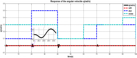
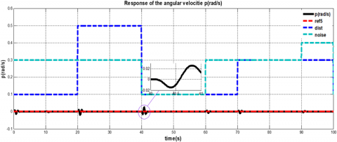
Figure 10 highlights the controller's competent performance in maintaining hovering flight, notwithstanding the impact of noise and disturbances (modeled as step values). In Figure 11, it is observed that the angular velocity is initially influenced by the introduction of noise and disturbances. However, the response swiftly corrects itself, tending towards zero, indicating effective disturbance rejection and system stabilization.
Figure 12 suggests that minor adjustments in translation velocities are necessary during Hover flight to ensure stability, underscoring the controller's adaptability.
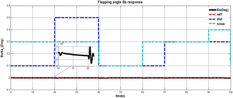
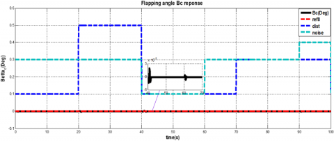
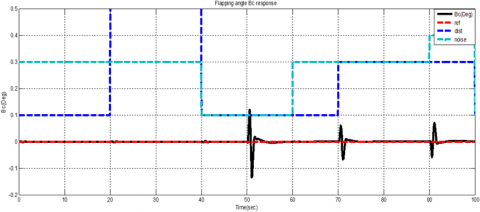
Figures 13(a) and (b) focus on the responses of the flapping angles BS and BC. These figures reveal that both angles remain close to zero, affirming the system's stability during hovering flight, even when subjected to external disturbances.
(a) Roll response
(b) pitch response
Figure 10. Responses of the attitudes
(a) Angular velocity $q=0$ response
(b) Angular velocity $p=0$ response
Figure 11. Responses of the angular velocities
(a) Linear velocity $u \approx 0$ response
(b)linear velocity $v \approx 0$ response
Figure 12. Responses of the linear velocities
(a) Flapping angle $B_S$ response
(b) Flapping angle $B_C$ response
Figure 13. Response of the flapping angles
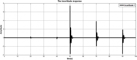
(a) Incertitude1 response
(b) Incertitude2 response
Figure 14. Response of incertitude for Hover
Finally, Figure 14 illustrates the impact of uncertainties on the system's responses, clearly showing that the introduction of disturbances and noise directly affects the response amplitude.
The step response of the controller, as shown in Figure 14, effectively minimizes the error between the desired outputs and inputs.
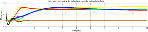
Figure 15 illustrates the helicopter's performance during hovering. It reaches the set point with minimal overshoot and settles effectively, corroborating the summarized results in Table 1. This demonstrates the controller's ability to maintain stability and control during hovering maneuvers, even in the presence of external disturbances or operational variations.
Figure 15. Unity step input tracking for $H_{\infty}$ optimal controller for Hover
Table 1. Transient performance of the USSH for step input
|
Parameters Response |
H∞ Controller Hover Flight |
H∞ Controller Translation Flight |
||||||
|
Theta |
Phi |
u |
v |
Theta |
Phi |
p |
q |
|
|
Rise time (s) |
l.75s |
1.75s |
0.39s |
0.49s |
1.71s |
1.85s |
2.01s |
1.83s |
|
Overshoot (%) |
14% |
14% |
27% |
17% |
14% |
14% |
14% |
14% |
|
Peak - time (s) |
4s |
4s |
0.99s |
1.23s |
4s |
4s |
4s |
4s |
4.2 Forward translation
$\left\{\begin{array}{l}x_1=\left[u q \theta v p \phi B_c B_s\right]^T \\ \theta_{\text {ref }}=0.6,0.5,0.7 \mathrm{rad} \\ \phi_{\text {ref }}=0.6,0.3,0.7 \mathrm{rad} \\ p_{\text {ref }}=0.6,0.3,0.7 \mathrm{rad} \\ q_{\text {ref }}=0.6,0.3,0.7 \mathrm{rad} \\ u_{\text {ref }}=10,20,10 \frac{\mathrm{m}}{\mathrm{s}} \\ v_{\text {ref }}=10,20,10 \frac{\mathrm{m}}{\mathrm{s}} \\ \bar{u}=\left[\delta_c \delta_a\right]^T \\ y_1=\left[u q \theta v p \phi B_c B_s\right]^T\end{array}\right.$ (36)
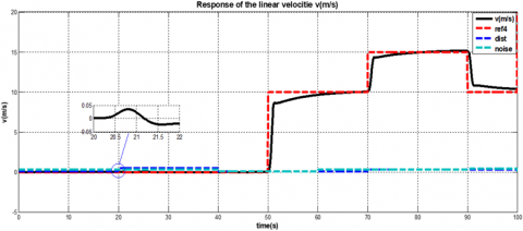
Figure 16 illustrates the linear velocity response for varying values of (u, v). This response indicates successful tracking, even amidst disturbances and noise, highlighting the controller's ability to maintain desired trajectories under challenging conditions.
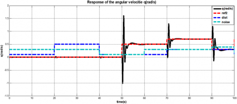
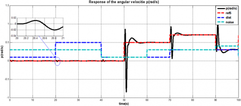
Figure 17 focuses on the angular velocity response. Notably, some oscillations are observed when the set point changes. However, the system quickly stabilizes, effectively following the set point despite these initial fluctuations. This quick stabilization demonstrates the controller's ability to handle dynamic changes in flight conditions.
Figure 18 presents the response of the roll and pitch angles. These angles closely follow the set points with only minor variations, which are attributed to the injection of noise and disturbances. This minimal deviation underlines the controller's precision in maintaining the desired attitude of the helicopter.
Figure 19 shows the responses of the flapping angles $B_S$ and $B_C$ during forward translational flight. Remarkably, both angles remain near zero, even when faced with external disturbances. This consistent behavior is a strong indicator of the system's stability during translational maneuvers.
Figure 20 is the impact of uncertainties on the system's responses and it is clear that the insertion of disturbances and the noise have a direct effect on its amplitude.
From these observations, it can be concluded that the controller not only ensures effective forward flight but also maintains stability in the face of uncertainties, noise, and disturbances. These results validate the robustness and reliability of the controller in managing both Hover and translational flight modes under a variety of operational conditions.
(a) Linear velocity u response
(b) Linear velocity v response
Figure 16. Responses of the linear velocities
(a) Angular velocity q response
(b) Angular velocity p response
Figure 17. Responses of the angular velocities
(a) Roll response
(b) pitch response
Figure 18. Responses of the attitudes
(a) Flapping angle $B_s$ response
(b) Flapping angle $B_C$ response
Figure 19. Response of the flapping angles
(a) Incertitude1 response
(b) Incertitude2 response
Figure 20. Response of incertitude for translation flight
Figure 21. Unity step input tracking for $H_{\infty}$ optimal controller for translation
The performance of the SSUH under the guidance of the optimal controller is quantitatively assessed through key metrics such as rise time, overshoot, and peak time. These metrics provide insight into the controller's efficiency and response characteristics during different flight maneuvers.
In Figure 21, the helicopter's forward translation is observed. The helicopter reaches the set point with an acceptable level of overshoot in linear velocity u and v. Notably, a lower overshoot is achieved with smaller step changes in the reference signals.
The objective of this research was to develop a robust optimal feedback controller to stabilize a SSUH and ensure precise trajectory tracking amid uncertainties and disturbances. The following key steps were undertaken:
1. The mathematical modeling of the SSUH was executed using Newton's approach, as opposed to the Euler-Lagrange method. The nonlinear system was linearized using Taylor approximation around an equilibrium point, identified as the hovering flight condition.
2. The nominal lateral-longitudinal linear model of the SSUH was derived, predicated on the assumption of a constant mass. This assumption excludes variations due to fuel consumption or payload offloading. Should this assumption be revised, the nominal linear model would need to incorporate parametric uncertainties resulting from mass variations. The present study did not consider shifts in the center of gravity or changes in the inertia tensor, focusing exclusively on mass-related parametric uncertainties.
3. Filter selection was meticulously conducted to ensure both the robustness and stability of the mixed-sensitivity H∞ controller.
Simulation results demonstrated that the optimal robust control system provided satisfactory trajectory tracking for both Hover and forward flight modes. The robustness of the control system, in terms of stability and performance under disturbances and noise, was emphatically validated. A robustness analysis highlighted the inherent trade-off between sensitivity and complementary sensitivity. It is noted that while much of the existing literature focuses on the hovering maneuver, this study extends the scope to include both hovering and forward translation flights, addressing input disturbances, noise, and parameter uncertainties. The resulting controller is not only optimal and robust but also guarantees precise tracking performance.
Future research could explore the integration of μ-analysis control, promising enhanced robustness, stability, and performance in the presence of structured uncertainties. A comparative study with the current controller could elucidate the efficacy of the μ-analysis approach. Additionally, reducing the controller's order and analyzing the consequent effects on the SSUH's behavior presents a worthwhile avenue for further investigation.
|
$X_u$ |
Partial differential equation with respect to $u\left(X_u=\frac{\partial X}{\partial u}\right)$. |
|
$W_2(s)$ |
Control sensitivity weight. |
|
$W_1(s)$ |
Sensitivity weight |
|
$F(s)$ |
Shor tha for the interconnection $F_l\left(M_{1_{\text {lat-long }}}(s), K(s)\right)$. |
|
$P 1(s)$ |
The uncertainty plant connected to the uncertainty $\Delta$ with the structure $\Delta$, which is equal to the connect $F_u\left(M_{1_{\text {lat-long }}}, \Delta\right)$. |
|
K(s) |
The controller. |
|
SSUH |
Small-Scale Unmanned Helicopter. |
|
$M_{1_{\text {lat-long }}}$ |
Nominal plant lateral longitudinal motion. |
|
Greek symbols |
|
|
$u, v, w$ |
Velocity components in $x, y$ and $z$ body axes system. |
|
$p, q, r$ |
Angular roll, pitch and yaw rates. |
|
$\phi, \theta, \psi$ |
Roll, pitch and yaw angles. |
|
$\delta_a$ |
Lateral cyclic pitch. |
|
$\delta_c$ |
Longitudinal cyclic pitch. |
|
$\delta_e$ |
Main rotor collective pitch. |
|
$\delta_p$ |
Tail rotor collective pitch. |
|
$\delta$ |
The uncertainty variable, $\delta \in[-1,1]$. |
|
$\beta_c$ |
Control rotor longitudinal tilt angle. |
|
$\beta_s$ |
Control rotor lateral tilt angle. |
[1] Gavrilets, V., Mettler, B., Feron, E. (2003). Dynamic model for a miniature aerobatic helicopter. Massachusetts Institute of Technology, MIT-LIDS report# LIDS-P-2579.
[2] Yechout, T., Morris, S.L., Bossert, D.E., Halgren, W.F. (2014). Introduction to Aircraft Flight Mechanics; American Institute of Aeronautics and Astronautics. Inc.: Reston, VA, USA.
[3] Wang, X., Chen, Y., Lu, G., Zhong, Y. (2015). Robust attitude tracking control of small-scale unmanned helicopter. International Journal of Systems Science, 46(8): 1472-1485. https://doi.org/10.1080/00207721.2013.822939
[4] Yu, B., Kim, S., Suk, J. (2019). Robust control based on ADRC and DOBC for small-scale helicopter. IFAC-PapersOnLine, 52(12): 140-145. https://doi.org/10.1016/j.ifacol.2019.11.183
[5] Ma, R., Ding, L., Liu, K., Wu, H. (2019). Dynamical model identification for a small-scale unmanned helicopter using an integrated approach. International Journal of Aerospace Engineering, 2019: 8407013. https://doi.org/10.1155/2019/8407013
[6] Choudhary, S.K. (2017). Optimal feedback control of a twin rotor MIMO system. International Journal of Modelling and Simulation, 37(1): 46-53. https://doi.org/10.1080/02286203.2016.1233008
[7] Khalesi, M.H., Salarieh, H., Saadat Foumani, M. (2020). System identification and robust attitude control of an unmanned helicopter using novel low-cost flight control system. Proceedings of the Institution of Mechanical Engineers, Part I: Journal of Systems and Control Engineering, 234(5): 634-645. https://doi.org/10.1177/0959651819869718
[8] Sahin, İ.H., Kasnakoğlu, C. (2015). An affine parameter dependent controller for an autonomous helicopter at different flight conditions. IFAC-PapersOnLine, 48(9): 174-179. https://doi.org/10.1016/j.ifacol.2015.08.079
[9] Yan, K., Chen, M., Wu, Q., Lu, K. (2019). Robust attitude fault-tolerant control for unmanned autonomous helicopter with flapping dynamics and actuator faults. Transactions of the Institute of Measurement and Control, 41(5): 1266-1277. https://doi.org/10.1177/0142331218775477
[10] Duan, X., Yue, C., Liu, H., Guo, H., Zhang, F. (2020). Attitude tracking control of small-scale unmanned helicopters using quaternion-based adaptive dynamic surface control. IEEE Access, 9: 10153-10165. https://doi.org/10.1109/ACCESS.2020.3043363
[11] Said, M., Larabi, M.S., Kherief, N.M. (2023). Robust control of a quadcopter using PID and H∞ controller. Turkish Journal of Electromechanics and Energy, 8(1): 3-11.
[12] Papalambrou, G., Karlis, E., Kyrtatos, N. (2015). Robust control of manifold air injection in a marine diesel engine. IFAC-PapersOnLine, 48(14): 438–443. http://doi.org/10.1016/j.ifacol.2015.09.496
[13] Doyle, J., Stein, G. (1981). Multivariable feedback design: Concepts for a classical/modern synthesis. IEEE transactions on Automatic Control, 26(1): 4-16. http://doi.org/10.1109/tac.1981.1102555
[14] Ding, L., Wu, H.T., Yao, Y. (2015). Chaotic artifcial bee colony algorithm for system identifcation of a small-scale unmanned helicopter. International Journal of Aerospace Engineering, 2015: 801874, https://doi.org/10.1155/2018/9897684
[15] Venkatesan, C. (2015). Fundamentals of Helicopter Dynamics, CRC Press, Taylor & Francis Group.
[16] Padfield, G.D. (1981). A theoretical model of helicopter flight mechanics for application to piloted simulation. RAE Technical Report 81048.
[17] Padfield, G.D. (1996). Helicopter Flight Dynamics: The Theory and Application of Flying Qualities and Simulation Modeling. John Wiley & Sons.
[18] Gavrilets, V., Mettler, B., Feron, E. (2001). Nonlinear model for a small-size acrobatic helicopter. In Proceedings of the AIAA Guidance, Navigation, and Control Conference and Exhibit, Montreal, Canada, pp. 6-9.
[19] Budiyono, A., Wibowo, S.S. (2007). Optimal tracking controller design for a small scale helicopter. Journal of Bionic Engineering, 4(4): 271–280. https://doi.org/10.1016/S1672-6529(07)60041-9
[20] Calise, A.J., Prasad, J.V.R., Munzinger, C. (1998). Development of a real-time flight simulator for an experimental model helicopter. Georgia Institue of Technology, School of Aerospace Engineering.
[21] Chen, R.T. (1980). Effects of primary rotor parameters on flapping dynamics. Technical Report, No. A-7777.
[22] Budiyono, A., Sudiyanto, T., Lesmana, H. (2008). First principle approach to modeling of small scale helicopter. arXiv preprint arXiv:0804.3895. https://doi.org/10.48550/arXiv.0804.3895.
[23] Kwakernaak, H. (2002). Mixed sensitivity design. IFAC Proceedings Volumes, 35(1): 61-66. https://doi.org/10.3182/20020721-6-ES-1901.01236.
[24] Sanjeewa, S.D.A., Parnichkun, M. (2019). Control of rotary double inverted pendulum system using mixed sensitivity H∞ controller. International Journal of Advanced Robotic Systems, 16(2). http://doi.org/10.1177/1729881419833273
[25] Kwakernaak, H. (1993). Robust control and H∞-optimization-tutorial paper. Automatica, 29(2): 255-273.
[26] Choudhary, S.K. (2014). Robust feedback control analysis of magnetic levitation system. WSEAS Transactions on Systems, 13(27): 285-291. http://doi.org/10.5281/zenodo.2590932.
[27] Alotaibi, J., Morales, R.M. (2018). Mixed-sensitivity h-infinity on-blade control. Proceedings of the 44th European Rotorcraft Forum, Delft, The Netherlands, pp 1-8.
[28] Zhou, K., Doyle, J.C., Glover, K. (1996). Robust and Optimal Control. PrenticeHall, Englewood Cliffs, NJ, USA.
[29] Zennir, Y., Larabi, M.S. (2017). Robust H∞ controller of a nonlinear unstable system: Robotics wrist. International Journal of Mathematical Models and Methods in Applied Sciences, 4: 273-278.