Salam Ibrahim Khather*![]() | Muhammed A. Ibrahim
| Muhammed A. Ibrahim![]() | Abdullah I. Abdullah
| Abdullah I. Abdullah![]()
© 2023 IIETA. This article is published by IIETA and is licensed under the CC BY 4.0 license (http://creativecommons.org/licenses/by/4.0/).
OPEN ACCESS
Nonlinear model predictive control (NMPC) has been recognized as an influential control strategy for intricate dynamical systems due to its superior performance over conventional linear control systems. The complexity associated with nonlinear dynamics is a recurring issue in a multitude of engineering applications, rendering the development of nonlinear models a challenging endeavor. The construction of such models, either through correlating input and output data or applying fundamental energy conservation laws, presents considerable difficulties. The absence of an effective model suitable for fundamental nonlinear processes is a marked deficiency, one that NMPCs are poised to address. NMPCs demonstrate a pronounced advantage over linear MPCs, particularly in managing the complexities and nonlinearities inherent in various systems. They exhibit efficacy in controlling nonlinear dynamics, including input/output constraints, objective functions, and computationally demanding optimization problems integral to real-time applications in process industries, power systems, and autonomous vehicular systems. This capability has prompted extensive research into nonlinear dynamics, thereby diminishing the disparity between the analysis of linear and nonlinear MPCs. This review provides a thorough examination of NMPCs, encompassing the fundamental principle, mathematical formulation, and various algorithms associated with NMPCs. A concise overview of NMPC applications, along with the challenges they pose, is also discussed.
nonlinear model predictive control, applications and performance analysis, nonlinear dynamics, control system, NMPC algorithms, applications
Model predictive control (MPC) is one of the progressive methods which can be used to control a process and optimize the performance [1]. MPCs were initially developed to overcome the drawbacks of single loop controllers which cannot provide desired performance under specified constraints. MPC techniques are appropriate for applications that require robust control of constrained multivariable processes [2]. Few applications that demand high performance do not require explicit pairing of input and output variables for controlling the process and hence the constraints are adopted directly into the system. This can result in the open-loop optimal control problem [3]. Present MPC techniques are designed as linear dynamic models and hence are termed in general as linear model predictive control (LMPC) [4]. LMPCs belong to the group of MPC techniques which uses linear models for predicting the dynamics of the system by considering the linear constraints of the input and state of the system [5].
It is assumed that the linearity of LMPCs simplify the design of the model and the controller [6]. Based on this assumption, several models have implemented LMPCs for controlling different processes [7, 8]. However, most of the processes are practically nonlinear which affects the control mechanism and application of LMPC techniques. In addition, applications that are highly nonlinear operate at a fixed operating point and moderately nonlinear techniques are characterized by larger operating points such as multivariable polymer reactors [9]. It must be noted that, even if the system is linear, the dynamics of the closed loop systems are nonlinear due to varying constraints. This factor motivated the researchers to develop nonlinear model predictive control (NMPC) systems which can be used to predict and optimize the nonlinear control processes [10].
In general, NMPCs are the MPC techniques which operate based on nonlinear and non-quadratic constraints. Although NMPCs enhance the process operation, the theoretical and practical problems are more challenging compared to linear MPCs. Most of the challenges are due to the nonlinear programs which need to be resolved to achieve better control over the process. In control engineering perspective, all real-time systems are inherently nonlinear due to the application specific requirements [11]. The nonlinear characteristics along with complex environmental regulation, high quality product specifications, rising demand for productivity, extensive operating conditions and economic considerations force the systems to operate near to the threshold level. In these conditions, linear systems cannot handle the dynamics of the system and nonlinear models come to the rescue. This lack of efficiency of linear models motivates the researchers to adopt NMPCs for controlling system operation [12].
1.1 Principle of NMPC
The concept of NMPCs is formulated as the iterative solution for solving open loop and closed loop control problems considering the input constraints and the system dynamics. The prominent advantage of NMPC is its ability to handle varying system constraints which can either be input or state variables. The schematic of NMPC is illustrated in Figure 1. The fundamental principle of NMPC is based on three main concepts: (a) The system model which uses a nonlinear model to estimate the future process in real time applications (b) the optimal control law for performing online computations using an optimal control sequence to improve the system’s performance and achieve the desired outcome (c) the receding horizon wherein the initial value of the control sequence is applied and the horizon is shifted by one instance and based on this the new sequences are calculated [13].
Figure 1. Block diagram of NMPC
A brief overview of the components of NMPC are discussed in below points:
(i) The System Model: The NMPC model is mainly used to formulate the law for controlling the system operation. It is essentially important to maintain the accuracy of the model to achieve a stable control. The structure and functioning of the NMPC model are highly flexible i.e., no strict restrictions are applied while designing the model. If complete information about the model is available then it can be expressed mathematically in the state space form. In other cases, if only partial information is available then a black box model can be used to represent the state of the system. In such scenarios, the model is accompanied with a fuzzy system or a neural network is implemented to estimate the model’s performance. Fuzzy systems use fuzzy logic or rules for making decisions. On the other hand, neural networks mimic the learning and decision-making processes of the human brain for making complex decisions.
As discussed previously, most of the systems are nonlinear and the open loop control of the NMPC model is as shown in Figure 1. In certain applications, the NMPC model incorporates an inbuilt inner control loop or an externally provided feedback controller. The inner control loop controls the specific task of the system and external controller is responsible for providing specific feedback to the system. The case mentioned in reference [14] used NMPC to enhance the process of the feedback controller by handling the uncertainties. The NMPC with external feedback improved the performance of the controller compared to the open loop NMPC controller without any feedback controller. In another case, the inner loop dynamics was considered while designing a flatness based MPC (FMPC) which considers the nonlinearity associated with the controlling process [15]. The FMPC improved the resistance of the system towards modeling errors and reduced the input time delays.
(ii) The Optimal Control Law: The NMPC model consists of an optimal input sequence denoted as u*(k) which is calculated as a result of the optimization problem in the control process [16]. The performance metrics are evaluated based on the cost index which is defined as follows:
$\begin{align} & J=\sum\limits_{j={{N}_{1}}}^{{{N}_{2}}}{{{p}_{k}}}{{\left\| \hat{y}(k+j\mid k)-{{y}_{d}}(k+j) \right\|}^{2}} \text{ }+\sum\limits_{j=1}^{{{N}_{\alpha }}}{{{q}_{k}}}\|\Delta u(k+j-1){{\|}^{2}}+{{J}_{1}} \\\end{align}$ (1)
The initial term ‘J’ is used to compute the square error between the estimated output yd (k+j) and the predicted future output $\hat{y}(k+j \mid k)$. The output is predicted based on the feedback obtained at an instant k. The feedback error is calculated over a specific prediction horizon which lies between N1 and N2 samples. The term ‘j’ is used to control the horizon window of Nu instances, where $(\Delta u(k)=u(k)-u(k-1))$. The terms pk and qk are defined as the weights of the terms J and j. The term J1 is defined as the cost function which considers various specifications while optimizing the cost coefficients. NMPCs are predominantly used in agreement with specifications such as variation in the input and state variables as shown in Eqs. (2) and (3) respectively.
U-<u(k)<U+ΔU-<Δu(k)<ΔU+ (2)
Y-<y(k)<Y+ΔY-<Δy(k)<ΔY+ (3)
The constraints defined in Eq. (2) considers the practical restrictions of the control system and constraints mentioned in Eq. (3) prevent the system to operate under unfavorable horizons. The term J is optimized to obtain a minimum value and is evaluated based on the decision variables which vary with respect to the control increment sequence as shown in Eq. (4).
[Δu(k), Δu(k+1), …, Δu(k+Nu-1)] (4)
(iii) The receding horizon: Receding horizon is a control strategy used for solving an optimization problem over a finite time horizon at each time step. The term “receding” refers that the problem is solved for updated time interval. In this technique, only the initial terms of the optimal sequence u* (k+j) are applied to the system. Correspondingly, the horizon will be shifted one level up in the next step and the optimization is repeated based on the newly obtained values [17]. Fundamentally, the shifting of horizons happens at each sampling level and the feedback information is obtained at each level [18]. Though this process generates feedback in the control loop for every instance at a predefined sampling rate, it increases the computational burden on the system since it requires a larger number of computational resources for implementation. However, the computational burden can be minimized by applying intermittent feedback. In simple words, the complexity of the system depends on the feedback techniques used to provide the information during optimization. In most of the cases, a basic low-pass filter is used as a feedback filter which significantly reduces the additive noise. This mechanism is employed in association with input-output models wherein the output is used for repressing the effect of steady state errors. The design of feedback filters for state space models can be more complicated since it is often a stack of filters used for estimating the derivatives of integrals. In case of errors, the system realigns itself to prevent the effect of prediction error and this process becomes more important in applications that require long-range predictions.
1.2 Properties of NMPC
The prominent characteristics of NMPC are as follows [19, 20]:
•Nonlinear models can be directly used for prediction in NMPCs.
•The input and state constraints are considered explicitly.
•The performance criteria in terms of specified time domain are augmented.
•NMPCs require a real-time solution to solve an open-loop control problem.
•NMPCs estimate the state of the system while making predictions. This property can be considered as an advantage or limitation of NMPC.
The direct application of nonlinear models can be beneficial if the details of the first principles of the NMPC model is available. The availability of first principle helps in enhancing the performance of the closed loop without much fine-tuning. In recent times, the first principle of NMPC can be assessed even before building the plant or a model and this process helps the applications that require detailed models based on first principle to maintain consistency and minimize the cost [21]. In certain cases, where the first principle is not available, it is practically not possible to obtain an efficient nonlinear model using identification techniques. In such cases, other control techniques such as LMPC models are employed [22]. The LMPC models apply the input as the solution to the optimal control problem which can either benefit or affect the model’s performance at the same time. Besides, LMPC models consider the input and the state constraint and directly apply them to the model. This makes it difficult to control the operations of the model. In addition, the cost minimization and the constraints of the model can be calibrated on-line without redesigning the controller. These aspects make it difficult to model nonlinear systems. In this context, the adoption of NMPCs gain huge significance for handling the uncertainties [23, 24] and constraints of the state and input.
The contributions of this review are summarized as follows:
•This review paper provides a systematic review of the nonlinear MPCs (NMPCs), its performance analysis and applications.
•This paper discusses the principle of NMPCs, properties, mathematical formulation, and algorithms.
•This study presents a detailed analysis of different optimization models used for optimizing the NMPCs and the state of art of evolutionary techniques used for enhancing the performance of NMPCs.
•This paper also discusses the recent trends, challenges and research gaps in the field of NMPCs.
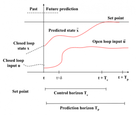
NMPCs are formulated as a repetitive solution for an open-loop control problem considering the state and input constraints along with system dynamics. The basic principle of NMPC is illustrated in Figure 2.
As shown in Figure 2, NMPC predicts the dynamic behavior of the control system by assessing the state of the model at time ‘t’. The behavior of the system in future is predicted over a horizon Tp and the input (between the horizon Tc≤Tp) is obtained to minimize the performance of the open-loop control system. If no disturbances and mismatches are observed in the model-plant, and if the plant operations can be modified over an infinite horizon, then the input signal at t=0 can be applied to the model-plant for all the values that are greater than 0 i.e., t≥0. In practical scenarios, the model-plant experiences disturbances and mismatches between the actual behavior of the system and predicted behavior. The error observed is transferred to the system via feedback and the open loop input (ū) is applied after the time interval (t+Tc) until the next set point is obtained.
Figure 2. Basic principle of NMPC
The sampling time required for optimizing the control problem can vary and the problem is re-evaluated after each sampling instance i.e., δ. At a time, instant t+δ, the system attains a new state and the future prediction and optimization of the control problem is performed again by shifting forward the horizon of the prediction and control system. As shown in Figure 2, the optimal open loop input (ū) is shown as an arbitrary function of time. In order to obtain an appropriate solution for the open loop control problem, the input (ū) is expressed in terms of fixed or finite parameters and thereby leads to a finite dimensional control problem. Practically, the control systems use a constant input and make Tc/δ decisions over the control horizon. The state of the input is determined based on the behavior of the predicted system and is measured as a function of different input and state constraints, with an aim to minimize the cost function. Since the behavior of the input in the open loop control system is predicted for a finite horizon, the behavior will be different from the closed loop system. This raises the concern about stability issues and necessary action should be taken to maintain the stability of the closed loop system and achieve closed loop desired performance.
Summarizing the principle of NMPC models, the process involved is as follows:
(i) Obtain prediction related to the state of the system for a finite horizon. This helps in making optimal control decisions even in the presence of nonlinearity and system perturbations. Predicting the state of the system over a finite horizon enable the NMPC system to address different critical aspects such as adapting to time-varying behavior of the system, mitigate the effect of disturbances, and ensure stability.
(ii) Evaluate the input function to minimize the cost function based on the predicted system model. The main advantage of minimizing the cost function is that it helps the NMPC system to achieve an optimal control over the system’s processes. The cost function is designed to control the performance of the system by controlling the input and minimization of cost function over a finite horizon enables the NMPC system to optimize the system’s behavior and there by improve the performance efficiency.
(iii) Implement one part of the input function until the next sampling instant is obtained. This helps in simplifying the process of understanding the impact of input and state constraints.
(iv) Repeat the process from step 2.
Considering a continuous system, the nonlinear differential equation can be described as follows:
$\dot{x}(t)=f((x), u(t)), x(0)=x_0$ (5)
Correspondingly, the input and state constraints are expressed as shown in Eqs. (6) and (7) respectively.
$u(t) \in \mathrm{U}, \forall t \geq 0$ (6)
$x(t) \in \mathrm{U}, \forall t \geq 0$ (7)
where, u(t)∈Rm and x(t)∈Rn represent the vector of inputs and states respectively.
With respect to these vectors, the constraint set for input U is considered to be compact and the constraints for system state X is considered to be connected. For instance, U and X are usually defined by the constraints that are defined in Eqs. (8) and (9) respectively.
$\mathrm{U}:=\{u \in R m \mid u \min \leq u \leq u \max \}$ (8)
$\mathrm{X}:=\{x \in R n \mid x \min \leq x \leq x \max \}$ (9)
where, umin, umax and xmin, xmax are the constant vectors. The input function in NMPCs is normally defined by the solution obtained for an open loop optimal control problem which is computed over a finite horizon at each sampling instant.
Some of the prominent aspects of NMPCs including different algorithms and approaches are discussed in this section which have gained huge prominence in the past decades.
Most of the linear dynamic systems are characterized by fundamental differential equations and algebraic equations. Linear systems describe the behavior of a controller which is characterized by linearity and time-invariance. As a result, problems related to NMPCs are formulated in a continuous time domain. An optimal control problem (OCP) in continuous time domain can be realized in an infinite dimensional space and it requires optimized parameters for converting the continuous time OCP into a nonlinear program (NLP). Techniques that first discretize the OCP and solve NLP in a finite dimension are defined as direct methods [25]. Two prominent algorithms that can be used to solve NLP are interior point (IP) methods and sequential quadratic programming (SQP) [26-28]. In order to extend the adaptability of NMPCs in various applications including dynamic approaches, and advanced versions of IP and SQP techniques, several techniques have been proposed with an aim to find optimal solutions for NLP [29-31]. For example, methods based on real-time iteration (RTI) execute one SQP iteration at a time and categorizes the calculations into two phases namely a preparation and feedback phase. This categorization is performed to apply the control input soon after the system’s states are measured. If the sampling time is less, then this method is used to evaluate the performance of the closed loop NMPC models [32]. As observed, both linear MPCs, NMPCs, and structured QP problems are solved using an iterative mechanism wherein the iterations are performed at each time step. Several algorithms and effective softwares are essential for solving NMPCs and there is a need to address the problems related to high computational overhead in traditional control systems. A significant amount of research work has been done in the field of NMPCs and have proposed different algorithms for exploiting the underlying problems associated with NMPCs.
As discussed previously, IP and SQP techniques are the two prominent algorithms which are predominantly used to solve nonlinear problems. In the IP method, the condition of non-smooth complementarity in the Karush– Kuhn–Tucker (KKT) system is modified and is interchanged with a smooth nonlinear approximation. The KKT system incorporates a set of important constraints for solving optimization problems, specifically problems involving both equality and inequality constraints. The KKT system helps in finding the solutions to these problems by analyzing the factors that are used for optimizing the performance. Solving KKT system is one of the fundamental approaches for finding optimal solutions in various optimization problems with constraints. In contrast, SQP techniques linearize the unequal constraints to find a point that can satisfy the optimal conditions for KKT and become equal to solve a quadratic problem. However, both these techniques follow a structured optimal control flow for solving QP. In general, SQP techniques use customized algorithms for addressing sub problems of QP and are advantageous in terms of warm-starting compared to IP techniques. Warm starting is the ability of an algorithm to make an ideal consideration for obtaining optimal solution and achieve convergence. Such considerations are already available in MPC-based approaches that obtain solutions based on the previous problem. On the other hand, IP-based techniques follow a central path, which reduces the effect of warm starting. Few solutions to overcome this problem are discussed by Zanelli et al. [33]. In NMPCs, the state of the system varies frequently while the controller calculates the next possible optimal input. In such cases, the RTI technique decreases the time between the control feedback and the measurement of the system's state by executing one SQP iteration per instance and by dividing the calculations into feedback and preparation phases. All these processes belong to the preparation phase and do not rely on the state measurements. The feedback phase consists of the initial values and solutions for QP sub problems for providing the feedback. While interpreting the results, there are chances that the state of the problem varies and can cause perturbations in the controller’s performance. This must be handled carefully such that the perturbations do not affect the performance of the closed loop system [34]. The RTI schemes developed for NMPC does not make use of any globalization strategy and assumes that all steps are required to achieve local convergence. Globalization strategies are the techniques used to ensure that the optimization algorithm converges to a feasible solution globally. These strategies focus on improving the reliability and performance of the NMPC controller. Both convergence and stability can be achieved by implementing a simple computation process with only a few required equality constraints that are discussed by Diehl et al. [35]. In order to decrease the computational burden, the RTI technique can further divide the calculations and process into multiple sub-levels and are operated with different frequencies. Initially, RTI method was the part of MUSCOD-II and was modified later and implemented in an ACADO Toolkit which is an open-source software tool. This toolkit provides both direct single and multiple shooting as parameterization techniques and various SQP algorithms and are integrated with qpOASES for obtaining solutions for dense sub problems of QPs. For embedded applications with sampling times (which is the range of microseconds), ACADO tool generates a code that can solve nonlinear problems. It consists of a RTI technique, with appropriate parameters to solve a nonlinear OCP using a Gauss–Newton Hessian approximation method. The code is generated for differential equations and for performing numerical simulations to improve the performance of the algorithms used for NMPCs. Several real-time algorithms implemented for NMPCs that are used for addressing nonlinear problems include Newton-type controllers [36]. This type of controllers performs one iteration of SQP per time instance using a Gauss–Newton Hessian. The Gauss–Newton Hessian is an optimization method used for solving the problem of nonlinear least squares. This method is analyzed with respect to the parameters being optimized and the main objective of this method is to find the best parameters for approximating the performance of the system.
However, a line search and a single shooting is used as an advanced controller which executes iterations for IP to achieve convergence and to reduce the delay. This is performed by estimating initial state constraints and implementing a tangential predictor to rectify the difference observed from the obtained measurements and the actual measurement of the system. Applying the Newton-type iteration with Gauss–Newton Hessian for single shooting can treat inequality issues in IP-based methods. Many techniques such as augmented Lagrangian-based techniques have been used in the existing literary works to solve the rising NLPs in a structured manner. In NMPCs that use input constraints, simple numerical techniques such as the projected gradient techniques, proximal techniques, and the projected Newton techniques are applied to achieve optimal solution.
IP techniques have several advantages such as ability to achieve global convergence while solving optimization problems, and has lower memory requirements. In addition, IP techniques use numerical approximation which makes it easy for solving the problem which are difficult to solve using direct methods. However, there are certain drawbacks which affects the performance of IP techniques. IP methods require a large number of iterations for converging compared to standard optimization techniques. It is challenging to update the parameters in IP-based NMPC systems because of high computational complexity. On the other hand, SQP techniques can handle equality constraints naturally and thereby make it convenient for solving NMPC problems with equality constraints. However, SQP techniques are more prone to get stuck in local optima and hence find it difficult to achieve global optimal solution.
It can be inferred from the study that IP methods are suitable for solving large-scale convex NMPC problems without relying on explicit derivatives and SQP techniques are more appropriate for solving fundamental convex problems with equality constraints that require fast convergence. The selection of these two techniques depends on the specific characteristics of the NMPC problem wherein there is a tradeoff between the local and global optimality and computational efficiency.
The theoretical aspects of NMPCs are essentially important to understand the stability issues of closed loop systems. In addition to the issue of closed loop system stability, the problems related to nominal stability of closed loop systems, different NMPC strategies, and their impact on the output feedback are also researched extensively. In real-time applications the NMPCs are considered as instantaneous NMPCs wherein it is assumed that the computational time required for evaluating optimal is nil and the instantaneous value δ=0. Here, the sample data of NMPC is used to calculate the optimal input value at different sampling instances. This section elaborates on different theoretical aspects of NMPC such as stability, infinite horizon, and finite horizon. Stability of NMPC is one of the critical aspects of closed-loop system which ensures that the behavior of the system under perturbations remains safe, steady, and predictable. Another important theoretical aspect of NMPC is infinite horizon which refers to a control strategy wherein the optimization problem is solved over an infinite time horizon. Infinite horizon in NMPC optimizes the controlling actions over an indefinite time space. The main objective of applying an infinite horizon in NMPC is to achieve a steady state behavior for a specific operating time. Finite horizon is another important theoretical aspect which enables a proper tradeoff between the control actions and computational complexity. By selecting an appropriate finite horizon for prediction, NMPC can realize real-time constraints and strengthen its ability to handle complex dynamic systems over a finite time period. A brief overview of these theoretical aspects is discussed in the sections below.
4.1 Stability of NMPC
The prominent aspect in NMPCs is to define whether the NMPC technique over a finite horizon can ensure the closed loop stability or not. The main issue in NMPCs with respect to predicting the outcome over the control horizon is due to the difference between the estimated open loop behavior and actual closed loop behavior. Fundamentally, an effective strategy is required to achieve closed loop stability which is independent of the parameters required and predicts the infinite horizon accurately. An effective NMPC technique which can ensure the stability of a closed loop is independent of the parameter selection and is termed as the NMPC technique which can guarantee stability of the NMPCs. Numerous strategies and techniques are used to stabilize closed loop systems using finite horizons. These strategies use only approximated parameters which are not validated practically. The technical evaluations can be performed based on certain assumptions which are independent of the application. Without generalization, it is considered that the origin of the state and input i.e., (x=0, u=0) is the steady state parameter used to stabilize the nonlinear system. In addition to this, the predictive horizon is equalized to the control horizon which is defined as Tp=Tc to simplify the stabilization process.
4.2 Infinite horizon NMPC
Applying an infinite horizon is one of the most effective methods to stabilize nonlinear MPCs. In this technique, the value of Tp is set to infinity (∞) and the trajectories of input and state constraints are considered as the solution for optimizing NMPC problems. These problems can be solved by defining a sampling instance which is equal to the trajectories of the closed loop nonlinear system. Therefore, the other samples of the trajectories at different sampling instances are considered to be optimal, which also defines the convergence of the closed loop system.
4.3 Finite horizon NMPC schemes with guaranteed stability
There exist several possibilities to achieve stability of the closed loop system over a finite horizon. Most of these techniques transform the conventional NMPC schemes in such a way that it ensures closed loop stability of nonlinear controllers. This can be achieved by including approximated equality and inequality constraints along with additional penalty parameters which can help in ensuring the stability. Equality constrains are the conditions which represent physical laws, dynamics of the system and other constraints which should be compulsorily satisfied at each time step within the finite horizon. These constraints define the relation between the predetermined state and input variables. On contrary, inequality constraints define the conditions which need not be satisfied compulsorily over a finite horizon. These constraints define the limits on the input and state variables in order to ensure that the stability of the system is not affected.
The additional penalty parameters are not affected by the physical limitations of system constraints and their only objective to ensure stability. Hence, these parameters are often considered as stability constraints. Another way of ensuring the stability of NMPCs over a finite horizon is to include an equality constraint with a zero terminal at the end of the predicted finite horizon. Similar to this, the possibility of applying one sampling instance at a time does not guarantee that all other sampling instances can contribute to improve stability. The main drawback of this possibility of applying a zero terminal is that the predicted state of the closed loop system is enforced to reach the origin within a fixed time. This raise concerns over the possibility of achieving stability for systems which short control horizon lengths or short prediction applications. In terms of computational feasibility, it is essential to satisfy the constraint of zero terminal equality which requires infinite iterations. This is not practical and hence is not suitable for real-time applications. However, the prominent advantage of zero terminal constraints is that it is very simple and is suitable for straightforward applications. Several existing works have studied the stability of NMPCs. Some of the works that studied the stability of NMPCs are tabulated in Table 1.
Table 1. Existing works on stability of NMPC
|
Reference |
Stability Analysis |
|
[37] |
The stability conditions for NMPC are analyzed with cyclically varying horizons. Structured terminal constraints and terminal penalties are considered to analyze the stability conditions. |
|
[38] |
The properties of nonlinear programming problems (NLPs) are explored to improve the stability and robustness of NMPCs |
|
[39] |
The partial stability analysis of NMPCs is analyzed by determining the behavior dynamic NMPC systems considering terminal costs and constraints |
|
[40] |
The inherent properties and robustness of NMPCs are analyzed to formulate economic NMPC. The study states that the system is practically stable even in the presence of disturbances |
|
[41] |
A long prediction horizon is provided to ensure stability of NMPC with desired output response. Results validate the practicability of the stability approach |
The robust characteristics of NMPCs in terms of achieving stability under the presence of system disturbances makes it an appropriate choice for the design of control systems. As discussed in previous sections, it is challenging to obtain an appropriate solution for optimizing the nonlinear problem at each sampling instance. In this context, various formulations are introduced which can prevent the problems related to optimization. Different optimization techniques have been designed for NMPCs in past decades to optimize the problems of NMPCs, which are discussed as follows.
5.1 Suboptimal NMPC
The suboptimal NMPCs eliminates the need for finding the minimum value of a non-convex cost function by assuming that satisfying the constraints for a nonlinear system is the preliminary consideration [42]. If the optimization technique can provide desired outcome at each sub-iteration (within a sampling instance) and can minimize the cost function then optimization can be terminated and an optimal solution can be obtained with robust stability. After applying the optimization strategy, the system continues to be stable even after the sampling time is over. It can be said that it is reliable to minimize cost function continuously in order to achieve stability. The optimization technique proposed by Chen et al. [43] used a metaheuristic based genetic algorithm (GA) for optimizing the control sequence in NMPCs. The main objective is to minimize the computational burden on NMPCs by obtaining a feasible solution rather than computing optimal solutions for each sample interval. The solution obtained reduces the cost function instead of minimizing it. This technique significantly lowers the computational time at every iteration without affecting the performance of the system. The low complexity attribute of the GA algorithm makes it practically feasible for real time control systems. Another suboptimal optimization approach is proposed by Berning Jr et al. [44] which aims to control the uncertainties and help the system to be stable. In addition, the computationally intensive NMPCs can be used to optimize the nonlinear problems without compromising on the performance of closed loop systems.
5.2 Simultaneous approach
Simultaneous approach is also termed as multiple shooting approach wherein the dynamics of the system at each sampling instance can be considered as nonlinear parameters for optimization [45]. In other words, an equality constraint should be satisfied for each sampling instance, as shown in below equation:
Ŝi+1=ŷ(ti+1,Ŝi,ûi) (10)
where, Ŝi is defined as an additional parameter used to solve optimization problem and can be used to determine the initial condition for each sampling instance ‘i’. After achieving convergence, all the trajectories of the system are aggregated together. Therefore, in addition to the input vector ûi {û1, û2, …, ûN}, the vector of Ŝi is also termed as the variable used for optimization. However, in both these techniques, the optimization problem can be solved using SQP methods. This method can be advantageous and possess certain drawbacks. For instance, the application of initial states Ŝi is considered as an effective optimization variable which can solve sparse behavior of the QP problem. This behavior can be considered to design a fast and robust strategy. The main disadvantage associated with the simultaneous approach is that it provides an appropriate state trajectory at the end of the iterative process. This increases the computational time and if the optimization is not completed on time, then it is not possible to ensure the possibility of the trajectory.
5.3 Application of short horizons
To achieve better computational performance, it is desired to apply short horizons since it reduces the required number of parameters and decision variables for optimization. However, it is feasible to implement long horizons for achieving satisfactory performance for closed loop systems. Multiple techniques are introduced to overcome the stability problem. In reference [46], a code generation strategy is proposed for managing short and long horizons in NMPCs. Existing RTI, QP, and condensing strategies are not suited for short horizons, and their execution time varies linearly with the increase in the length of the horizon. Correspondingly, Ławryńczuk and Nebeluk [47] proposed an algorithm which integrates all relevant features for optimizing the cost function. The main motive behind this approach is to reduce the computational load and to calculate the first step of the actual control sequence. In addition, the first step is required to estimate the remaining variables of the control sequence which is not calculated. Here, the required number of decision variables does not depend on the control horizon. This is feasible only if there is no sufficient time for calculating the complete control sequence and calculate only the first variable and predict the rest of the variables. An optimization algorithm that incorporates a single degree of freedom was implemented previously for NMPC based control systems. The optimization function is obtained by performing interpolation between the control law and a suboptimal control law. Here, the control law is considered as the absence of constraints (though it is not contributing to the stability of the system) and a suboptimal control law is directly related to the stability concerns. The interpolation between these two laws generates desired optimality and stability and the control law used for stabilization incorporates a single degree of freedom and can be executed by imposing an appropriate penalty on the convergence requirements and the cost function.
5.4 Decomposition of the control sequence
The prominent advantage of linear MPC systems is the implementation of free and forced response. This process is not well-suited for NMPC applications and as a result, the principle of superposition cannot be applied for this case. This concept can be transformed and then implemented for formulating NMPCs. In certain applications, predicting the system’s output can be carried out by including the free response of NMPCs and by adding the forced response from the linear model of the control system. The estimations are made in such a way that the response can be approximated due to the principle of superposition, which allows the division or decomposition of the control sequence into smaller segments and is applied only to linear systems. In addition, the estimation made in this way can be a better solution than the solutions obtained using a linear model for computing the output response. This problem can be resolved by manipulating the control sequence and the variables and such manipulated sequence can be used along with the fundamental control sequence and a series of control sequences with the manipulated parameters. The output of the process ‘j’ can be predicted and is calculated as the sum of the output of the process (yb(t+j)) and due to the incremented input sequences in addition to the response of the system (yi(t+j)), the future control sequence can be calculated. In this approach the responses from both linear and nonlinear models are used for computation wherein, the term (yb(t+j)) is used as a computation obtained from nonlinear model, while the term (yi(t+j)) is used as a computation obtained from a linear model of the control system. Correspondingly, the cost function is formulated as a quadratic function for all the decision variables and can be used to solve the QP sub problem as a linear MPC. Similar to the linear MPC, the principle of superposition cannot be applied for nonlinear systems. The output response obtained from the nonlinear system will align with the output response obtained from the linear MPC system, only if the sequence of the future variables is 0. If the output response does not align with each other, then the fundamental value is made equal to the last value of the control sequence along with the optimized control increment obtained by the QP algorithm. The same process is repeated until all the sequence of the future control sequence is set to zero.
5.5 Feedback linearization
For linearizing the feedback, the nonlinear MPC system can be converted to a linear MPC model by approximating the transformations. However, this is feasible only in certain cases and this does not hold good for all the cases. A sample instance for transforming nonlinear MPC into linear MPC is given as follows:
Consider a nonlinear system whose process is determined using the state space model as shown in Eq. (11).
$x(t+1)=f(x(t)), u(t) y(t)=g(x(t))$ (11)
where, x(t+1) is the input sequence at a time instance t+1, u(t) is the initial state, y(t) is the output sequence and g(x(t)) is the future control sequence. The process of determining the input and state transformation functions denoted as: $z(t)=h(x(t))$ and $u(t)=p(x(t), v(t))$. The term is modified as shown in Eq. (12).
$z(t+1)=A z(t)+B v(t) y(t)=C z(t)$ (12)
However, the linearization method is often characterized by two prominent limitations. The first drawback is associated with the transformation functions that can be computed only for certain cases and are not suitable for all cases. The second drawback is related to the constraints of the system which are mostly linear and can be converted into a different set of nonlinear constraints.
In summary, the optimization techniques can ensure the stability of NMPCs by solving complex problems. It can be inferred that the suboptimal NMPC techniques do not ensure that global optimal solution. Instead, these techniques converge to a local optimum which is not the best solution for optimizing the control objectives. In certain cases, the suboptimal techniques have a negative impact on the performance of the NMPC systems compared to global optimization methods. Hence these methods are not suitable for applications that rely on global solutions. The simultaneous approaches are computationally intensive and are not effective in real-time control applications. Although short horizon-based methods achieve excellent results in terms of improving the computational performance, they cannot capture the behavior of the system for a longer period and this drawback can reduce the performance efficiency of the system in a longer run. In addition, the limited predictive capability fails to capture the dynamics of the complex system under long term disturbances. Thereby these techniques do not exhibit desired performance in applications that require a longer prediction horizon to achieve high performance. Furthermore, the process involved in the decomposition-based methods and the feedback linearization methods are not appropriate for all applications.
Numerous applications have implemented different control systems based on NMPC. This section discusses some of the prominent control system designs for different applications.
An advanced control algorithm based on NMPC for a variable speed wind turbine is presented by Dang et al. [48] for controlling the speed of the shaft to capture power at different speed levels and maintain the power level below the maximum level during high wind speed. Due to the drawbacks of power electronic converters, the torque generated is also kept below the maximum value. The dynamic system constraints are controlled by the NMPC algorithm which is considered as a potential solution by the researchers. The efficacy of the NMPC algorithm in regulating the speed of the turbine is validated through simulation. A NMPC based controlling system is proposed for thermal management (TM) in Plug-in Hybrid Electric Vehicles (PHEVs) is implemented by Lopez-Sanz et al. [49]. One of the important drawbacks associated with the TM process is the high energy consumption due to the increase in the count of low voltage components used for cooling processes. More complicated and advanced control techniques are required for reducing the number of components in TM and simultaneously reduce the energy consumption in PHEVs. In such cases, NMPCs act as a potential tool for solving multi objective problems in Multiple input- Multiple output (MIMO) systems. The NMPC proposed in this work for the TM and power electronic circuits in a PHEV is highly effective and is highly distinguishable from previous NMPC approaches in the domain of PHEVs. The complexity of the nonlinear control plants which are perturbed by the nonlinearity is reduced by controlling the system variables. Results show that the NMPC techniques reduce the power consumption by 5% approximately and optimizes the objective function and improves the performance by 30%. A similar approach based on traction control is presented by Tavernini et al. [50]. In the control system, the feedback law was obtained before and the variations in the system constraints with respect to different plant conditions were discussed. The explicit controller is used for controlling the prototyping unit and strengthens the performance of the controller by improving the computation time which is in the range of microseconds. The performance is compared with the explicit NMPCs along with a proportional integral (PI)-based traction controller. The performance is compared with one implicit NMPC and two explicit NMPCs for different control models by considering the transient behavior and without considering the load transfers. Results of the experimental evaluations show that explicit NMPCs are more suitable for improving the performance of the electric vehicles. With the advancements in the controlling strategies, NMPCs are also accompanied with artificial intelligence (AI) based techniques such as neural networks and deep learning models. A multi-level NMPC is used as controller by Lucia and Karg [51] which are employed for learning the policy of robust NMPCs using deep learning based deep neural networks (DNN). The implementation of NMPCs with DNN is based on the fact that deep learning (DL) models achieve phenomenal results in terms of improving the representation capabilities of the DNN compared to shallow learning models. The experimentation process validates the effectiveness of the DNN with several hidden layers incorporated to achieve a better process. On the other hand, shallow models do not achieve desired performance when used with multiple hidden layers. Results show that the DNN model improves the learning capabilities of the NMPCs. A similar approach is presented by Karg and Lucia [52] wherein a combined form of moving horizon estimation (MHE) and NMPC is considered to be more robust and stable not only because of its formulation but also its ability to solve two optimization problems at a time. However, this can be a complex task due to the time and resource constraints. In this research, the advantages of the DNN are exploited to obtain an optimal solution for both MHE and NMPC problems. The computational load is reduced by replacing the MHE constraints with the NMPC based on the learning aspects. Karg and Lucia [53] implemented a reinforced learning based robust NMPC control approach. The controllers designed using this approach is also known as imitation learning and have some significant limitations which makes it difficult for learning the behavior of the system which is not represented well and must be reevaluated by designing from the beginning once the controlling strategy changes. These drawbacks are addressed by integrating two factors such as imitation learning and the learning attributes of the reinforcement learning (RL) algorithm. The main objective behind this work is to make an effective use of the control policy which is updated after every iteration using reinforcement learning. RL-based models can learn dynamically from the previous instances. In addition, the advantages of the RL algorithm make it easy to approximate the NMPC and the efficiency of combining two learning concepts is highlighted in this work and is validated through simulation results. The existing research works have validated the effectiveness of the DL based NMPCs in terms of optimizing the nonlinear problems and achieving better control over the system’s performance.
Despite the advantages of NMPCs offered to enhance the stability of the closed loop control systems, there are certain challenges that restrict the performance efficiency of the NMPCs. This research identifies some of the prominent challenges, which can be summarized as follows:
•It is difficult to solve highly nonlinear problems due to the constraints and difficulty in formulating the economic objectives in NMPCs.
•The design of an effective nonlinear model is essential to accurately capture the intricate phenomena in the control systems and it is complicated to design such systems.
•It is challenging to achieve a balanced tradeoff between tracking and correcting steady-state errors. This problem can be addressed by modifying the controller architecture, which is a difficult task.
•There is a need for a deeper analysis which can focus on the stability and robustness of the NMPCs and this problem gets worsened when applied for open loop unstable systems.
These challenges must be addressed effectively to increase the adaptability of the NMPCs to different applications. For further research, the study of NMPCs can be extended to solve the issue of stability in open loop unstable control systems. As inferred from existing research works, there is a limited focus on the review of NMPCs as more focus is given to the linear and conventional MPCs. In addition, it is also necessary to identify different types of open loop unstable control systems wherein NMPCs can be studied based on the specific concepts. These points contribute as a potential research gap which can be considered as directions for future research.
This paper emphasizes the study of NMPCs and its performance in different applications. NMPCs are most suitable for solving the nonlinear problems in control systems. Studies reveal that the design of NMPCs for different controllers is a difficult task and more advanced control strategies are required for addressing this complexity. A brief overview of the theoretical aspects and optimization of NMPCs using different techniques is presented in this paper. In addition, the application of NMPCs for different applications is discussed and the prominent observations are recorded. The prominent observations of this research can be summarized as follows:
NMPCs can effectively handle highly nonlinear dynamics, constraints, and uncertainties, which are persistent in modern engineering and control applications.Algorithms such as IP and SQP techniques are used to solve optimization problems in NMPCs by achieving global convergence. The performance analysis demonstrates the effectiveness of NMPC in achieving superior control objectives and its ability to handle challenging control scenarios.
The paper also outlines prominent research challenges as observed from the existing literary works and identifies the research gap for further research.
|
MPC |
Model predictive control |
|
NMPCs |
Nonlinear MPC |
|
LMPC |
Linear model predictive control |
|
OCP |
Optimal control problem |
|
NLP |
Nonlinear program |
|
SQP |
Sequential quadratic programming |
|
RTI |
Real-time iteration |
|
KKT |
Karush-Kuhn-Tucker |
|
TM |
Thermal management |
|
PHEVs |
Plug-in Hybrid Electric Vehicles |
|
MIMO |
Multiple input- Multiple output |
|
PI |
Proportional integral |
|
AI |
Artificial intelligence |
|
DNN |
Deep neural networks |
|
DL |
Deep learning |
|
MHE |
Moving horizon estimation |
|
RL |
Reinforcement learning |
[1] Kouvaritakis, B., Cannon, M. (2016). Model Predictive Control. Switzerland: Springer International Publishing.
[2] Li, X., Zhao, Z., Liu, F. (2020). Latent variable iterative learning model predictive control for multivariable control of batch processes. Journal of Process Control, 94: 1-11. https://doi.org/10.1016/j.jprocont.2020.08.001
[3] Dontchev, A. L., Kolmanovsky, I.V., Krastanov, M.I., Veliova, V.M. (2020). Approximating open-loop and closed-loop optimal control by model predictive control. In 2020 European Control Conference (ECC), St. Petersburg, Russia, pp. 190-195. https://doi.org/10.23919/ECC51009.2020.9143615
[4] Ostadijafari, M., Dubey, A. (2019). Linear model-predictive controller (LMPC) for building’s heating ventilation and air conditioning (HVAC) system. In 2019 IEEE Conference on Control Technology and Applications (CCTA), Hong Kong, China, pp. 617-623. https://doi.org/10.1109/CCTA.2019.8920657
[5] Rosolia, U., Borrelli, F. (2017). Learning model predictive control for iterative tasks: A computationally efficient approach for linear system. IFAC-PapersOnLine, 50(1): 3142-3147. https://doi.org/10.1016/j.ifacol.2017.08.324
[6] Rosolia, U., Borrelli, F. (2019). Sample-based learning model predictive control for linear uncertain systems. In 2019 IEEE 58th Conference on Decision and Control (CDC), Nice, France, pp. 2702-2707. https://doi.org/10.1109/CDC40024.2019.9030270
[7] Narasingam, A., Kwon, J.S.I. (2019). Koopman Lyapunov‐based model predictive control of nonlinear chemical process systems. AIChE Journal, 65(11): e16743. https://doi.org/10.1002/aic.16743
[8] Bai, G., Meng, Y., Liu, L., Luo, W., Gu, Q., Liu, L. (2019). Review and comparison of path tracking based on model predictive control. Electronics, 8(10): 1077. https://doi.org/10.3390/electronics8101077
[9] Li, S., Li, Y. (2016). Model predictive control of an intensified continuous reactor using a neural network Wiener model. Neurocomputing, 185: 93-104. https://doi.org/10.1016/j.neucom.2015.12.048
[10] Lucia, S., Andersson, J.A., Brandt, H., Diehl, M., Engell, S. (2014). Handling uncertainty in economic nonlinear model predictive control: A comparative case study. Journal of Process Control, 24(8): 1247-1259. https://doi.org/10.1016/j.jprocont.2014.05.008
[11] Wang, P., Zhang, B., Su, H. (2018). Stabilization of stochastic uncertain complex-valued delayed networks via a periodically intermittent nonlinear control. IEEE Transactions on Systems, Man, and Cybernetics: Systems, 49(3): 649-662. https://doi.org/10.1109/TSMC.2018.2818129
[12] Reichensdörfer, E., Odenthal, D., Wollherr, D. (2018). On the stability of nonlinear wheel-slip zero dynamics in traction control systems. IEEE Transactions on Control Systems Technology, 28(2): 489-504. https://doi.org/10.1109/TCST.2018.2880932
[13] Allgöwer, F., Zheng, A. (Eds.). (2012). Nonlinear Model Predictive Control (Vol. 26). Birkhäuser.
[14] Lucia, S., Finkler, T., Basak, D., Engell, S. (2012). A new robust NMPC scheme and its application to a semi-batch reactor example. IFAC Proceedings Volumes, 45(15): 69-74. https://doi.org/10.3182/20120710-4-SG-2026.00035
[15] Greeff, M., Schoellig, A.P. (2018). Flatness-based model predictive control for quadrotor trajectory tracking. In 2018 IEEE/RSJ International Conference on Intelligent Robots and Systems (IROS), Madrid, Spain, pp. 6740-6745. https://doi.org/10.1109/IROS.2018.8594012
[16] Grüne, L., Pannek, J. (2017). Nonlinear model predictive control. Nonlinear Model Predictive Control, pp. 45-69. https://doi.org/10.1007/978-3-319-46024-6_3
[17] Grüne, L. (2013). Economic receding horizon control without terminal constraints. Automatica, 49(3): 725-734. https://doi.org/10.1016/j.automatica.2012.12.003
[18] Mesbah, A., Streif, S., Findeisen, R., Braatz, R.D. (2014). Stochastic nonlinear model predictive control with probabilistic constraints. In 2014 American Control Conference, Portland, OR, USA, pp. 2413-2419. https://doi.org/10.1109/ACC.2014.6858851
[19] Alamir, M. (2014). Fast NMPC: A reality-steered paradigm: Key properties of fast NMPC algorithms. In 2014 European Control Conference (ECC), Strasbourg, France, pp. 2472-2477. https://doi.org/10.1109/ECC.2014.6862620
[20] Nurkanović, A., Zanelli, A., Albrecht, S., Frison, G., Diehl, M. (2020). Contraction properties of the advanced step real-time iteration for NMPC. IFAC-PapersOnLine, 53(2): 7041-7048. https://doi.org/10.1016/j.ifacol.2020.12.449
[21] Brásio, A.S., Romanenko, A., Fernandes, N.C., Santos, L.O. (2016). First principle modeling and predictive control of a continuous biodiesel plant. Journal of Process Control, 47: 11-21. https://doi.org/10.1016/j.jprocont.2016.09.003
[22] Hafez, A.T., Iskandarani, M., Givigi, S.N., Yousefi, S., Rabbath, C.A., Beaulieu, A. (2014). Using linear model predictive control via feedback linearization for dynamic encirclement. In 2014 American Control Conference, Portland, OR, USA, pp. 3868-3873. https://doi.org/10.1109/ACC.2014.6858619
[23] Ersdal, A.M., Imsland, L. (2017). Scenario-based approaches for handling uncertainty in MPC for power system frequency control. IFAC-PapersOnLine, 50(1): 5529-5535. https://doi.org/10.1016/j.ifacol.2017.08.1094
[24] Yu, S., Reble, M., Chen, H., Allgöwer, F. (2014). Inherent robustness properties of quasi-infinite horizon nonlinear model predictive control. Automatica, 50(9): 2269-2280. https://doi.org/10.1016/j.automatica.2014.07.014
[25] Verschueren, R., van Duijkeren, N., Quirynen, R., Diehl, M. (2016). Exploiting convexity in direct optimal control: A sequential convex quadratic programming method. In 2016 IEEE 55th Conference on Decision and Control (CDC), Las Vegas, NV, USA, pp. 1099-1104. https://doi.org/10.1109/CDC.2016.7798414
[26] Zavala, V.M., Laird, C.D., Biegler, L.T. (2008). Interior-point decomposition approaches for parallel solution of large-scale nonlinear parameter estimation problems. Chemical Engineering Science, 63(19): 4834-4845. https://doi.org/10.1016/j.ces.2007.05.022
[27] Diehl, M., Ferreau, H.J., Haverbeke, N. (2009). Efficient numerical methods for nonlinear MPC and moving horizon estimation. Nonlinear Model Predictive Control: Towards New Challenging Applications, pp. 391-417. https://doi.org/10.1007/978-3-642-01094-1_32
[28] Kirches, C., Bock, H.G., Schlöder, J.P., Sager, S. (2011). Block-structured quadratic programming for the direct multiple shooting method for optimal control. Optimization Methods & Software, 26(2): 239-257. https://doi.org/10.1080/10556781003623891
[29] Ohtsuka, T. (2004). A continuation/GMRES method for fast computation of nonlinear receding horizon control. Automatica, 40(4): 563-574. https://doi.org/10.1016/j.automatica.2003.11.005
[30] Hult, R., Zanon, M., Frison, G., Gros, S., Falcone, P. (2020). Experimental validation of a semi‐distributed sequential quadratic programming method for optimal coordination of automated vehicles at intersections. Optimal Control Applications and Methods, 41(4): 1068-1096. https://doi.org/10.1002/oca.2592
[31] Astudillo, A., Gillis, J., Diehl, M., Decré, W., Pipeleers, G., Swevers, J. (2022). Position and orientation tunnel-following NMPC of robot manipulators based on symbolic linearization in sequential convex quadratic programming. IEEE Robotics and Automation Letters, 7(2): 2867-2874. https://doi.org/10.1109/LRA.2022.3142396
[32] Diehl, M., Bock, H.G., Schlöder, J.P. (2005). A real-time iteration scheme for nonlinear optimization in optimal feedback control. SIAM Journal on Control and Optimization, 43(5): 1714-1736. https://doi.org/10.1137/S0363012902400713
[33] Zanelli, A., Quirynen, R., Jerez, J., Diehl, M. (2017). A homotopy-based nonlinear interior-point method for NMPC. IFAC-PapersOnLine, 50(1): 13188-13193. https://doi.org/10.1016/j.ifacol.2017.08.2175
[34] Ding, X.C., Schild, A., Egerstedt, M., Lunze, J. (2009). Real-time optimal feedback control of switched autonomous systems. IFAC Proceedings Volumes, 42(17): 108-113. https://doi.org/10.3182/20090916-3-ES-3003.00020
[35] Diehl, M., Findeisen, R., Allgöwer, F. (2007). A stabilizing real-time implementation of nonlinear model predictive control. In Real-Time PDE-Constrained Optimization, pp. 25-52. https://doi.org/10.1137/1.9780898718935.ch2
[36] Deng, H., Ohtsuka, T. (2019). A parallel Newton-type method for nonlinear model predictive control. Automatica, 109: 108560. https://doi.org/10.1016/j.automatica.2019.108560
[37] Kögel, M., Findeisen, R. (2013). Stability of NMPC with cyclic horizons. IFAC Proceedings Volumes, 46(23): 809-814. https://doi.org/10.3182/20130904-3-FR-2041.00184
[38] Yang, X., Griffith, D.W., Biegler, L.T. (2015). Nonlinear programming properties for stable and robust NMPC. IFAC-PapersOnLine, 48(23): 388-397. https://doi.org/10.1016/j.ifacol.2015.11.310
[39] La, H.C., Potschka, A., Bock, H.G. (2017). Partial stability for nonlinear model predictive control. Automatica, 78: 14-19. https://doi.org/10.1016/j.automatica.2016.11.047
[40] Griffith, D.W., Zavala, V.M., Biegler, L.T. (2017). Robustly stable economic NMPC for non-dissipative stage costs. Journal of Process Control, 57: 116-126. https://doi.org/10.1016/j.jprocont.2017.06.016
[41] Köhler, J., Zeilinger, M.N., Grüne, L. (2023). Stability and performance analysis of NMPC: Detectable stage costs and general terminal costs. IEEE Transactions on Automatic Control. https://doi.org/10.1109/TAC.2023.3235244
[42] García, J.J.V., Garay, V.G., Gordo, E.I., Fano, F.A., Sukia, M.L. (2012). Intelligent multi-objective nonlinear model predictive control (iMO-NMPC): Towards the ‘on-line’ optimization of highly complex control problems. Expert Systems with Applications, 39(7): 6527-6540. https://doi.org/10.1016/j.eswa.2011.12.052
[43] Chen, W., Li, X., Chen, M. (2009). Suboptimal nonlinear model predictive control based on genetic algorithm. In 2009 Third International Symposium on Intelligent Information Technology Application Workshops, Nanchang, China, pp. 119-124. https://doi.org/10.1109/IITAW.2009.46
[44] Berning Jr, A.W., Liao-McPherson, D., Girard, A., Kolmanovsky, I. (2020). Suboptimal nonlinear model predictive control strategies for tracking near rectilinear halo orbits. arXiv Preprint, arXiv:2008.09240.
[45] Diangelakis, N.A., Burnak, B., Katz, J., Pistikopoulos, E.N. (2017). Process design and control optimization: A simultaneous approach by multi‐parametric programming. AIChE Journal, 63(11): 4827-4846. https://doi.org/10.1002/aic.15825
[46] Vukov, M., Domahidi, A., Ferreau, H.J., Morari, M., Diehl, M. (2013). Auto-generated algorithms for nonlinear model predictive control on long and on short horizons. In 52nd IEEE Conference on Decision and Control, Firenze, Italy, pp. 5113-5118. https://doi.org/10.1109/CDC.2013.6760692
[47] Ławryńczuk, M., Nebeluk, R. (2021). Computationally efficient nonlinear model predictive control using the L1 cost-function. Sensors, 21(17): 5835. https://doi.org/10.3390/s21175835
[48] Dang, D.Q., Wang, Y., Cai, W. (2008). Nonlinear model predictive control (NMPC) of fixed pitch variable speed wind turbine. In 2008 IEEE International Conference on Sustainable Energy Technologies, Singapore, pp. 29-33. https://doi.org/10.1109/ICSET.2008.4746967
[49] Lopez-Sanz, J., Ocampo-Martinez, C., Alvarez-Florez, J., et al. (2016). Nonlinear model predictive control for thermal management in plug-in hybrid electric vehicles. IEEE Transactions on Vehicular Technology, 66(5): 3632-3644. https://doi.org/10.1109/TVT.2016.2597242
[50] Tavernini, D., Metzler, M., Gruber, P., Sorniotti, A. (2018). Explicit nonlinear model predictive control for electric vehicle traction control. IEEE Transactions on Control Systems Technology, 27(4): 1438-1451. https://doi.org/10.1109/TCST.2018.2837097
[51] Lucia, S., Karg, B. (2018). A deep learning-based approach to robust nonlinear model predictive control. IFAC-PapersOnLine, 51(20): 511-516. https://doi.org/10.1016/j.ifacol.2018.11.038
[52] Karg, B., Lucia, S. (2021a). Approximate moving horizon estimation and robust nonlinear model predictive control via deep learning. Computers & Chemical Engineering, 148: 107266. https://doi.org/10.1016/j.compchemeng.2021.107266
[53] Karg, B., Lucia, S. (2021b). Reinforced approximate robust nonlinear model predictive control. In 2021 23rd International Conference on Process Control (PC), Strbske Pleso, Slovakia, pp. 149-156. https://doi.org/10.1109/PC52310.2021.9447448