Taha S. Mahmood* | Omar F. Lutfy
© 2022 IIETA. This article is published by IIETA and is licensed under the CC BY 4.0 license (http://creativecommons.org/licenses/by/4.0/).
OPEN ACCESS
As a powerful nonlinear control design strategy, feedback linearization provides viable design tools for a wide range of nonlinear systems. This paper presents an intelligent feedback linearization design using the inverse feedforward control (IFC) scheme to control nonlinear dynamical systems. Particularly, the nonlinear autoregressive moving average (NARMA-L2) network is trained to reproduce the controlled system's forward dynamics. Consequently, the trained NARMA-L2 network can be directly employed in the IFC structure. To enhance the approximation ability of the NARMA-L2 structure, two wavelet neural networks (WNNs) are utilized to constitute the NARMA-L2 controller. Moreover, the RASP1 function was utilized as the mother wavelet function instead of the commonly employed Mexican hat function. To avoid the limitations of the gradient descent (GD) methods, the genetic algorithm has been used as the training method to optimize the NARMA-L2 inverse controller parameters. The simulation results showed that the proposed controller was effective in terms of precise control and robustness against external disturbances. Furthermore, a comparison study with other control structures revealed that the control results of the proposed WNN-based NARMA-L2 controller with the RASP1 function are superior to those of the WNN-based NARMA-L2 with the Mexican hat function, the multilayer perceptron (MLP)-based NARMA-L2 controller, and the PID controller.
NARMA-L2, wavelet neural network, feedback linearization, inverse feedforward control, genetic algorithm, multilayer perceptron, PID controller
The use of intelligent techniques in dynamical system modeling and control has attracted the attention of many researchers. These techniques mimic the human ability to recognize objects and make decisions, and they are extremely beneficial in the design of powerful control structures. In this regard, the model structure to be used in the control algorithm must acquire major properties of the controlled system. However, this model should not complicate the design with a heavy processing burden. In particular, a suitable choice of the system model results in effective control and high efficiency. In this context, the nonlinear autoregressive moving average (NARMA-L2) model, introduced by Narendra and Mukhopadhyay [1], represents a simple, yet effective method to reproduce the dynamics of nonlinear systems. The NARMA-L2 model has the ability to transform nonlinear system dynamics into linear dynamics by canceling the nonlinearities. Therefore, it is most suited for the feedback linearization control [2].
To this end, several studies on NARMA-L2 controllers have been reported in the literature. For instance, the authors [3] used a NARMA-L2 structure to control a bioreactor and demonstrated that the trajectory tracking performance obtained was superior to that obtained with the inverse neural model control strategy. They employed a backpropagation algorithm (BPA) to obtain the optimal NN weights. Hamidi et al. [4] proposed a hybrid neural network to construct the NARMA-L2 structure using a multilayer perceptron (MLP) NN that can be used as a model for controlling a nonlinear (multi-input multi-output) MIMO quadcopter system. The BPA was used in order to find the best weights for the neural network. Moreover, Rashad [5] used the NARMA-L2 to control the speed of a permanent magnet DC motor, where a dynamic BPA was used to minimize the mean square of errors. In this regard, the performance of the NARMA-L2 controller is directly linked to the accuracy of the system’s model estimation. The BPA has been exploited in the majority of the NARMA-L2 applications reported earlier. However, the gradient descent-based BPA has a potential to become stuck at local minima and stop working. For this reason, evolutionary algorithms, such as genetic algorithms (GAs), have attracted much attention because of their ability to find the global solution to a particular problem. Consequently, several researchers used GA to design the NARMA-L2 controller [6, 7].
In the design of the IFC structure, an effective inverse model of the system to be controlled should be developed. The neural network is one of the best methods for dealing with IFC design requirements. The NNs have long been known to be powerful universal approximators [8-10]. Following that, the neural network-based inverse controller has seen a widespread application in the control of nonlinear systems. In this context, most researchers employed the MLP and the RBF NNs for the IFC structure. For example, Pedro et al. [11] proposed an MLP-based NARMA-L2 to control the slip in an anti-lock braking system. An internal model control (IMC) scheme using MLP has been used to control unknown nonlinear systems [12]. The IMC structure was utilized in this method with two filters including a set-point filter and a robustness filter. Because these filters use modifiable parameters that should be properly chosen, the precision of this approach may be limited.
In recent years, researchers have become increasingly interested in wavelet neural networks (WNNs), which integrate the wavelet and NN theories into a more powerful structure. These networks have the ability to learn and generalize like conventional NN, but they also have the ability to localize like a wavelet transform [13, 14]. The structure of WNNs has been shown to be better than those of other types of NNs due to its ability to add new mapping relationships between inputs and outputs [15]. To this end, the simulation results of this paper will show that the WNN outperforms the MLP in the IFC structure. Despite the WNN's appealing features, few researchers used the WNN as an inverse controller. For example, to control a nonlinear system, two WNNs have been used in the IFC scheme [16]. However, there were two training phases needed for this control method: one phase to identify a forward plant model and a second one to develop the inverse controller. Moreover, only few researchers used the WNN within the NARMA-L2 structure. For instance, Jin et al. [17], the authors applied the WNN based on the NARMA-L2 model to predict the thermal characteristics of a feed system. Lutfy and Selamat [18], a WNN-based NARMA-L2 was used for the IMC scheme to control nonlinear systems. However, this control method required two NARMA-L2 structures, which adds an additional computational burden. In addition, Alwan [19] employed a WNN-based NARMA-L2 for the IFC structure using the Mexican hat function as the mother wavelet function. The author employed the BPA to obtain the optimal NN weights. However, the main drawbacks of BPAs are their tendency to become trapped in the local minima of their search spaces and the difficulty in deciding the optimal setting for the learning coefficient.
In this paper, a WNN-based NARMA-L2 is proposed to act as an inverse feedforward controller to control nonlinear systems. The genetic algorithm is used as the training method to optimize the WNN weights. This control approach requires only one NARMA-L2 for acquiring the forward dynamics of the system. Subsequently, the control algorithm can be used right away without any more training. From the simulation results of controlling three nonlinear systems, the proposed control approach achieved the desired control objectives in terms of control accuracy and robustness despite the difference between the training and the testing signals for all the plants, which clearly indicates the remarkable generalization ability of the controller. Moreover, the GA has minimized the objective function from the early stage of the optimization process for the three plants. The organization of this paper can be summarized as follows: Section 2 describes the WNN-based NARMA-L2 network's structure. The genetic algorithm is discussed in detail in Section 3. Section 4 presents several performance and comparison tests to demonstrate the effectiveness of the proposed NARMA-L2 in the IFC scheme. Finally, in Section 5, the conclusions are drawn.
The neural network is an extremely powerful mathematical tool for solving problems involving nonlinear modeling. As a result, the nonlinear IFC structure in this study is designed using the NN [18]. Specifically, the NARMA-L2 network is used, which is a very effective NN structure [20]. The basic concept of this control strategy is to create an inverse controller in the IFC structure using a forward WNN-based NARMA-L2 model of the system to be controlled. The following sections cover the WNN's structure and the design process in detail.
2.1 Wavelet neural network structure
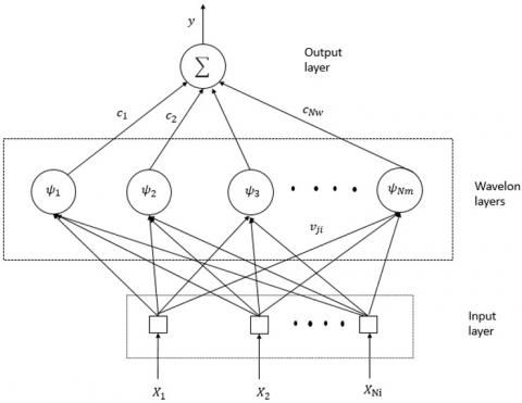
The WNN structure used in this work is illustrated in Figure 1, and it consists of three layers: an input layer, a mother wavelet (wavelon) layer, and an output layer. The role of each layer is described below [18, 21]:
Figure 1. Structure of the WNN
Layer 1: It is the input layer that accepts the input variables $\left(x_1, x_2, \ldots, x_{N i}\right)$ and sends them to the next layer.
Layer 2: It is the wavelon layer which is composed of mother wavelet nodes, also known as the "wavelons". In this study, rather than the commonly used Mexican hat function, the RASP1 function was used. In this regard, it was found that the RASP1 function surpasses other functions in terms of approximation performance after multiple experiments with other wavelet functions [22]. The following equation represents this function [23]:
$\psi(x)=\frac{x}{\left(1+x^2\right)^2}$ (1)
The formula below is utilized to determine the jth wavelon node's output in this layer [18]:
$\psi_i(x)=\psi\left(z_i\right)$, with $z_j=d_i\left(\sum_{i=1}^{N i} v_{j i} x_i\right)-t_i$ (2)
where, tj and dj denote the wavelet's translation and dilation factors, respectively, vji denotes the weight of the ith connection between the input layer and the jth wavelon in the mother wavelet layer, xi represents the ith input variable, and Ni denotes the input layer's node number. The final response of wavelon j is:
$\psi\left(z_j\right)=\frac{z}{\left(1+z^2\right)^2}$ (3)
Layer 3: This layer utilizes the following equation to compute the WNN's final output [21].
$y=\sum_{i=1}^{N w} c_j \psi_j(x)$ (4)
where, $N w$ is the nodes’ number in the wavelon layer and $c_j$ denotes a weight between the jth node and the output node.
Based on the previous discussion, there are various adjustable parameters to be tuned in the WNN structure. More specifically, the following set represents these parameters:
$M=\left[c_j d_j t_j v_{j i}\right]$, (5)
where, M denotes the collection of adjustable parameters. It is necessary to employ an appropriate optimization approach to optimize the parameters in Eq. (5) to obtain the best performance possible from the WNN structure. These parameters are established in the current study using the genetic algorithm, which will be discussed in more detail in the next sections.
2.2 The controller design utilizing the NARMA-L2 structure
The NARMA-L2 structure employed in this study requires two steps to be utilized; the system identification stage and the controller design stage. The NARMA-L2 network is formed by combining two WNN sub-networks that are trained utilizing the plant’s input-output data during the system identification stage. The purpose is to obtain a NARMA-L2 model of the system that will be used for control. During the stage of controller design, the controller is made by rearranging the two sub-networks that were trained in the system identification process to make the controller. In order to ensure that the plant output follows the reference input, the following control input is calculated using a mathematical formula [20]. To this end, the controller represents controlled plant's inverse dynamics. As a result, the invertibility of the plant to be controlled is a major consideration in this design approach [18].
2.2.1 The forward system identification stage of NARMA-L2 Using the WNN
The equation below describes the general structure of the NARMA-L2 model [20]:
$\begin{aligned} y(k+1)=f(& y(k), y(k-1), \ldots, y(k-n\\ &+1), u(k-1), \ldots, u(k-m\\ &+1)) \\ &+g(y(k), y(k-1), \ldots, y(k\\ &-n+1), u(k-1), \ldots, u(k\\ &-m+1)) \cdot u(k) \end{aligned}$ (6)
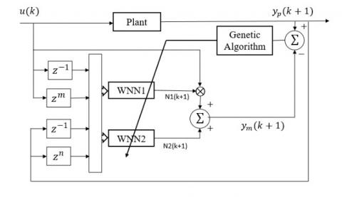
In this study, two WNNs are utilized to approximate the NARMA-L2 network's two functions f and g. As depicted in Figure 2, the NARMA-L2 forward system identification stage uses a series-parallel identification structure. The modeling error $e_m(k+1)$ between the output of NARMA-L2 $y_m(k+1)$ and the actual system output $y_p(k+1)$ is subsequently utilized to optimize the NARMA-L2 model. The output of the NARMA-L2 is expressed in the equation below [18]:
$\begin{aligned} y_m(k+1)=\hat{f}(& y_p(k), y_p(k-1), \ldots, y_p(k-n\\ &+1), u(k-1), \ldots, u(k-m\\ &+1)) \\ &+\hat{g}\left(y_p(k), y_p(k\right.\\ &-1), \ldots, y_p(k-n+1), u(k\\ &-1), \ldots, u(k-m+1)) \cdot u(k) \end{aligned}$ (7)
To train the NARMA-L2 model, a quadratic cost function is employed in the genetic algorithm. This cost function is made up of the following:
$J=\frac{1}{N_P} \sum_{K=1}^{N_P}\left(y_p(k)-y_m(k)\right)^2$, (8)
where, ym(k) represents the output of the NARMA-L2, $y_p(k)$ represent the plant output, and Np represents the number of training patterns. Following a predetermined number of generations, the GA adjusts all the weights that can be modified in the WNN-based NARMA-L2 by minimizing Eq. (8).
Figure 2. WNN-based NARMA-L2 identification model
2.2.2 Controller design stage
It is necessary to form an inverse feedforward controller after creating the NARMA-L2 model. In this step, all that needs to be done is to use the developed NARMA-L2 model according to Eq. (7) to implement the controller. As previously mentioned, the NARMA-L2 system identification stage defined the functions $\hat{f}$ and $\hat{g}$ in Eq. (7). Furthermore, to ensure that the output of system $y_p(k+1)$ tracks the reference signal $y_r(k+1)$ , the following is done: $y_p(k+1)=y_r(k+1)$. Consequently, the final NARMA-L2 control action is generated as given below [20].
$u(k)=\frac{-\hat{f}\left[\begin{array}{c}y_r(k+1) \\ y_p(k), y_p(k-1), \ldots, \\ y_p(k-n+1), u(k-1), \ldots, \\ u(k-n+1)\end{array}\right]}{\hat{g}\left[\begin{array}{c}y_p(k), y_p(k-1), \ldots, \\ y_p(k-n+1), u(k-1), \ldots \\ u(k-n+1)\end{array}\right]}$ (9)
2.3 The general structure of the WNN-based NARMA-L2 inverse feedforward controller
Figure 3 illustrates the general WNN-based NARMA-L2 IFC scheme [19]. The robustness filter shown in Figure 3 adds robustness to the IFC structure to handle the errors made in the modeling of the structure. Additionally, it smooths out fast changing signals to enhance the IFC controller's transient response. The following is the equation for the robustness filter [19]:
$\frac{y_{\operatorname{ref}}(z)}{y_{\operatorname{des}}(z)}=\frac{1-\alpha}{1-\alpha z^{-1}}$ (10)
where, α is a tuning parameter.
Figure 3. WNN-based NARMA-L2 IFC structure
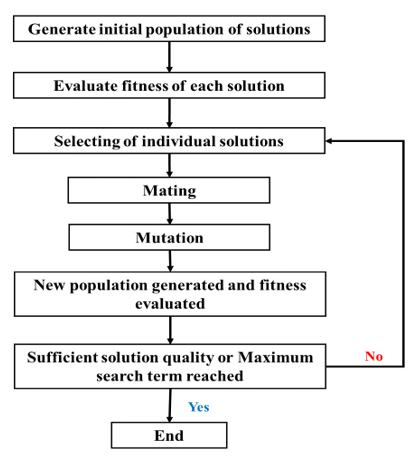
In the last few years, artificial intelligence techniques have become the most common way to solve many optimization problems. Genetic Algorithms (GAs) were utilized to solve various problems in the science and engineering fields [24]. Many modern evolutionary algorithms are directly based on genetic algorithms or have some strong similarities [25].
The GA is a random-guided optimization method that adopts the idea of survival of the fittest. It became popular in the early 1970s because of John Holland's work. The GA is part of a group of algorithms called evolutionary algorithms (EAs) that try to solve the problems of optimization through the use of natural evolution-inspired techniques [26]. The GA looks for the best solution in the search space from multiple directions, in contrast to classical search algorithms that employ local derivatives and progress in a single direction towards the optimal solution. There is a good chance that classical techniques which use the gradient method will get stuck in local minima. The GA, on the other hand, changes the genetic information of an offspring randomly to avoid this problem. The GA, on the other hand, changes the genetic information of an offspring randomly to avoid this problem. This means that the GA is always working with a group of solutions. This problem has a "fitness value" for each member of the group, which is based on the task's objective. Members that show better solutions are given more points for fitness, which helps them stay alive through the generations. In GAs, the first population is chosen at random, and then the genetic operator's of reproduction, crossover, and mutation are used to make new populations over time. These generations would come up with better solutions to the problem, and they would get closer and closer to the best solution over time [26]. Figure 4 illustrates a flowchart of the GA.
The following procedure illustrates the fundamental steps of the GA [25]:
Figure 4. Flowchart of the GA
This section examines the control results of the suggested WNN-based NARMA-L2 IFC structure optimized by the GA. Three nonlinear systems' modeling and control results are discussed in detail. Additionally, a disturbance rejection study was done to assess how well the proposed intelligent control method can handle disturbances. Furthermore, a comparison study with other control structures revealed that the control results of the proposed WNN-based NARMA-L2 controller with the RASP1 function are superior to those of the WNN-based NARMA-L2 controller with the Mexican hat function, the multilayer perceptron (MLP)-based NARMA-L2 controller, and the PID controller. In the genetic algorithm, the maximum number of generations was set to 1000, the crossover probability was set to 0.8, and the probability of mutation was set to 0.05 for all the controlled systems. Finally, for all the simulation tests, the filter’s parameter (α) was adjusted to a value of 0.3. In this work, the above settings were adequate to give the best control results.
4.1 Performance tests of control
The goal of these tests is to assess the applicability of the WNN-based NARMA-L2 IFC scheme to control the nonlinear plants below.
Plant 1:
The following is the differential equation for this nonlinear plant [19]
$y_p(k)$ $=0.35\left[\frac{y_p(k-1) y_p(k-2)\left(y_p(k-1)+2.5\right)}{1+y_p(k-1)^2+y_p(k-2)^2}\right.$ $+u(k-1)]$ (11)
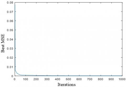
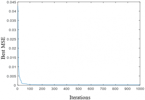
The controlled plant's WNN-based NARMA-L2 forward model must be developed in the first step of designing the IFC scheme. For this purpose, a training set of 500 input-output data points were produced utilizing a random input signal $u(k)$. To minimize the MSE criterion, the GA optimized the WNN-based NARRMA-L2 parameters utilizing the series-parallel identification structure illustrated in Figure 2. The training MSE was $7.66 \times 10^{-5}$ after 1000 iterations, as shown in Figure 5a, which shows the decrease in the MSE against 1000 iterations. To illustrate how quickly the GA was able to achieve convergence, see Figure 5a, which shows how the GA minimized the MSE from the beginning of the optimization processes. It has been decided to use a different signal for testing in order to assess the accuracy of the trained WNN-based NARMA-L2 network's modeling. Particularly, the signal of testing is defined according to the following equation [18]:
$u(k)=0.5 \sin \left(\frac{2 \pi k}{25}\right)+0.5 \sin \left(\frac{2 \pi k}{10}\right)$ (12)
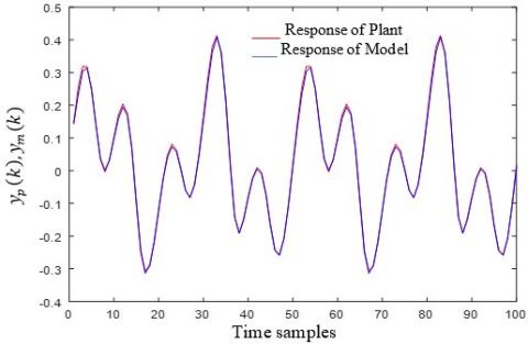
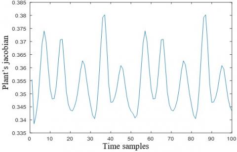
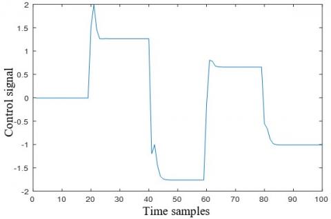
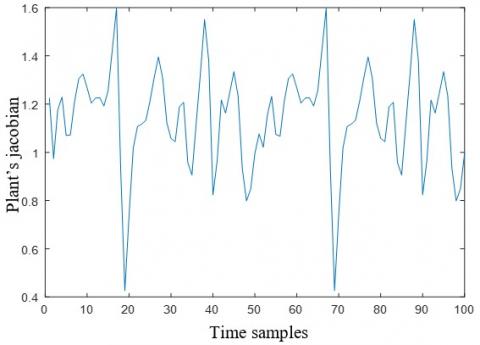
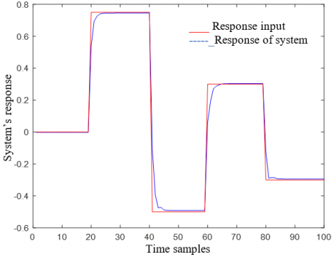
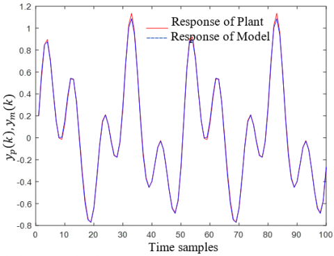
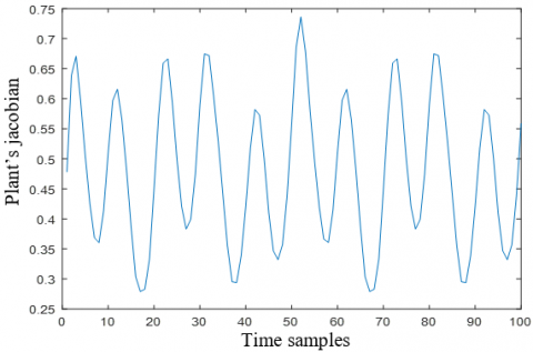
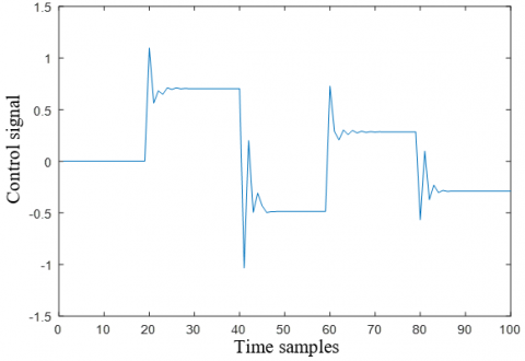
The modeling result shown in Figure 5b was obtained using the testing signal. The purpose of this testing signal, which is different from the random training signal, is to assess the generalization ability of the controller. We can see that the trained network has done an excellent job in tracking the testing signal with a MSE of $3.36 \times 10^{-5}$. Given that the NARMA-L2 was able to successfully track a signal that differed totally from the random signal used during the training phase, this modeling result shows that the WNN-based NARMA-L2 possesses a powerful generalization capability. In order to create an IFC controller, you must first determine if the plant model can be inverted. A simple way to check this is to check the Jacobin plant's signs in the area of interest. Figure 5c shows that the plant Jacobin is sign-definite, which means that the plant model can be constructed as an inverse controller in an IFC scheme. Therefore, the plant model is invertible. As shown in Figure 5d, the IFC scheme is able to track a step-changing signal with excellent control performance, and the resulting control signal is shown in Figure 5e.
(a) Finest MSE against iterations
(b) Plant and the WNN-based NARMA-L2 outputs
(c) the Jacobian of the plant
(d) the output response
(e) the control signal
Figure 5. (a-e) Simulation graphs for plant 1
Plant 2:
This plant represents a nonlinear discrete-time system as described by the equation below [19]:
$\mathrm{y}(\mathrm{k}+1)=\frac{1.5 y(k) y(k-1)}{1+y^2(k)+y^2(k-1)}$$+0.1 \times \sin (\mathrm{y}(\mathrm{k})+\mathrm{y}(\mathrm{k}-1))$$+1.2 \mathrm{u}(\mathrm{k})$ (13)
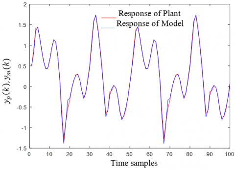
Controlling Plant 2 was accomplished using the same steps described for Plant 1. To begin, we utilized a random input signal $u(k)$ to develop the WNN-based NARMAL2 model. Figure 6a illustrates the decrease in the MSE as a function of the number of iterations that the genetic algorithm achieves after a few initial iterations. Specifically, the training MSE was $1.38 \times 10^{-4}$ after 1000 iterations. In order to evaluate the trained NARMA-L2 model, the testing signal of Eq. (12) was employed, and the result is shown in Figure 6b, demonstrating excellent accuracy for the testing signal with an MSE of $5.80 \times 10^{-3}$. Once more, the WNN-based NARMA-L2 showed superior performance because it was able to generalize its learning to follow a testing signal that did not exist throughout the training process. The plant model is invertible, as illustrated in Figure 6c. The IFC's control performance is demonstrated in Figure 6d, which shows excellent control accuracy. Figure 6e depicts the control action.
Plant 3:
This plant represents the Jacketed Stirred Reactor, also known as a Continuously Stirred Tank Reactor (CSTR). The following nonlinear difference equation shows the dynamics of this process [27]:
$\mathrm{y}(\mathrm{k}+1)=0.7653 \mathrm{y}(\mathrm{k})-0.231 \mathrm{y}(\mathrm{k}-1)$$-0.6407 y^2(\mathrm{k})+1.014 \mathrm{y}(\mathrm{k}-1) \mathrm{y}(\mathrm{k})$$\quad-0.3921 y^2(\mathrm{k}-1)+0.4801 \mathrm{u}(\mathrm{k})$$+0.592 \mathrm{y}(\mathrm{k}) \mathrm{u}(\mathrm{k})-0.5611 \mathrm{y}(\mathrm{k}-1) \mathrm{u}(\mathrm{k})$ (14)
(a) Finest MSE against iterations
(b) Plant and the WNN-based NARMA-L2 outputs
(c) The Jacobian of the plant
(d) The output response
(e) The control signal
Figure 6. (a-e) Simulation graphs for plant 2
(a) Finest MSE against iterations
(b) Plant and the WNN-based NARMA-L2 outputs
(c) The Jacobian of the plant
(d) The output response
(e) The control signal
Figure 7. (a-e) Simulation graphs for plant 3
The CSTR process is controlled using the same design process as the previous plants. Figure 7a illustrates the decrease in the MSE as a function of the number of iterations that the genetic algorithm achieves after a few initial iterations. More precisely, the training MSE was $2.93 \times 10^{-4}$ after 1000 iterations. To validate the generalization ability of the trained network, the signal of Eq. (12) was utilized. The resulting modeling performance is shown in Figure 7b, which demonstrates excellent modeling of the testing signal with an MSE of $2.25 \times 10^{-4}$. As illustrated in Figure 7c, the plant model is invertible. The IFC's control performance is illustrated in Figure 7d, which demonstrates remarkable output accuracy with just a few overshoots at each reference signal change. Figure 7e illustrates the controller output.
4.2 Disturbance rejection tests
To examine how well the proposed IFC scheme could deal with outside disturbances, a small-amplitude disturbance was injected into each plant's output for two periods; specifically $20 \leq k \leq 25$ and $70 \leq k \leq 75$ for all controlled plants. These disturbances were not applied during the IFC training phase. This adds extra difficulty to the IFC structure in handling unknown disturbances in the testing phase. As shown in Figure 8, the WNN-based NARMA-L2 IFC structure could handle the unexpected disturbances for the three plants.
4.3 A comparison study of the WNN and the MLP neural networks
In this section, comparison studies were carried out to assess the performance of the WNN and the MLP as the primary networks in the IFC structure trained by the GA. In this regard, the MLP is made with the same IFC structure explained in Sections 2.2 and 2.3. With respect to the MLP, two MLP networks were used, each of which is composed of three layers: the input layer, the hidden layer, and the output layer. Six hidden nodes with sigmoid activation functions make up the hidden layer and the output layer is made up of a single node that employs a linear activation function.
Owing to the stochastic nature of the GA, the output of a particular run may differ from the output of other runs. Thus, in order to perform an accurate comparison, ten runs were conducted in the NARMA-L2 IFC scheme for each network, including the WNN with the RASP1 function, the WNN with the Mexican Hat function, and the MLP. After that, the average of these ten runs can be used to calculate the performance of the three networks. Table 1 summarizes the results of the comparisons made in Section 4.1 for Plants 1, 2, and 3. Table 1 clearly demonstrates that the WNN with the RASP1 function outperforms the WNN with the Mexican Hat function and the MLP networks within the IFC scheme. Particularly, the WNN with the RASP1 function has achieved the lowest MSE values for both training and testing in terms of modeling precision. Furthermore, the WNN with the RASP1 function has the smallest integral square error (ISEs) values in terms of control accuracy. Finally, the WNN with the RASP1 function had the shortest processing time of the three plants.
(a) Plant_1
(b) Plant_2
(c) Plant_3
Figure 8. (a-c) Testing of Plants 1, 2, and 3 for disturbances Rejection
Table 1. The results of the performance comparison of the MLP, the WNN with the Mexican Hat function, and the WNN with the RASP1 function as the primary networks in the IFC structure
|
Type of networks |
Criterions (average of 10 runs) |
Controlled plants |
||
|
Plant 1 |
Plant 2 |
Plant 3 |
||
|
MLP |
Training MSE |
6.60E-04 |
2.08E-03 |
3.97E-04 |
|
Testing MSE |
2.43E-04 |
7.58E-03 |
5.02E-04 |
|
|
ISE |
3.449 |
3.636 |
3.46 |
|
|
Time (s) |
71.745 |
72.039 |
71.38 |
|
|
WNN with the Mexican Hat function |
Training MSE |
4.98E-04 |
4.19E-04 |
3.21E-04 |
|
Testing MSE |
1.52E-04 |
7.05E-03 |
4.67E-04 |
|
|
ISE |
3.4712 |
3.4761 |
3.454 |
|
|
Time (s) |
76.299 |
76.923 |
76.31 |
|
|
WNN with the RASP1 function |
Training MSE |
1.86E-04 |
2.03E-04 |
3.02E-04 |
|
Testing MSE |
5.37E-05 |
4.50E-03 |
4.43E-04 |
|
|
ISE |
3.425 |
3.4090 |
3.453 |
|
|
Time (s) |
67.96 |
69.70 |
69.35 |
|
Table 2. The results of the comparison of the PID controller and the WNN-based NARMA-L2 with the RASP1 function
|
Type of networks |
Criterions (average of 10 runs) |
Controlled plants |
||
|
Plant 1 |
Plant 2 |
Plant 3 |
||
|
PID |
ISE |
4.553 |
5.587 |
4.989 |
|
WNN with the RASP1 function |
ISE |
3.425 |
3.409 |
3.453 |
4.4 A comparison study with other control structures
The WNN-based NARMA-L2 IFC's performance is compared to that of the PID controller in this section. The GA optimizes the two controllers using the same plants as previously considered. In order to do a good comparison study, ten runs were done on each plant to get an average result. Table 2 shows that the WNN-based NARMA-L2 IFC structure has achieved better control results compared to the PID controller, which has resulted in an unacceptable steady-state error in the output response, as shown in Figure 9.
Figure 9. The output response of the PID controller
The purpose of this work is to develop and implement an intelligent control strategy for dynamical nonlinear systems based on the NARMA-L2 IFC scheme. The NARMA-L2 has the significant advantage of eliminating the nonlinear system's dynamic behavior. It is capable of converting a nonlinear dynamical system to an implied algebraic model, which makes it easier and more efficient to control the system's trajectory. Without the use of derivatives, the effort of control is calculated directly from the position reference. To overcome the limitations of the commonly used gradient methods, the weights of the WNN-based NARMA-L2 network have been optimized using the GA. Rapid convergence was achieved for all controlled plants using this optimization method by significantly reducing the MSE from the start of the optimization process. The main contributions of this work are the improved approximation ability of the WNN-based NARMA-L2 and the use of the GA rather than the widely used GD methods in previous studies. The proposed intelligent IFC structure's effectiveness in controlling nonlinear plants has been demonstrated through simulation results in terms of precise control performance and robustness against outside disturbances. Additionally, a comparison study with other control structures revealed that the proposed WNN-based NARMA-L2 controller with the RASP1 function outperforms the WNN-based NARMA-L2 controller with the Mexican hat function, the MLP-based NARMA-L2 controller, and the PID controller in terms of control results. The main requirement in the proposed method is that the controlled system should be invertible.
For future work, the proposed controller will be applied to control a real-time system using an adaptive control approach. This can significantly enhance the control performance of real-time industrial systems.
[1] Narendra, K.S., Mukhopadhyay, S. (1997). Adaptive control using neural networks and approximate models. IEEE Transactions on Neural Networks, 8(3): 475-485. https://doi.org/10.1109/72.572089
[2] Jibril, M., Tadese, M., Alemayehu, E. (2020). Tank liquid level control using NARMA-L2 and MPC controllers. Researcher Journal, 12(7): 23-27. https://doi.org/10.14293/S2199-1006.1.SOR-.PP5K4PY.v1
[3] Fourati, F., Baklouti, S., Moalla, H. (2015). NARMA-L2 neural control of a bioreactor. In 2015 4th International Conference on Systems and Control (ICSC), pp. 504-509. https://doi.org/10.1109/ICoSC.2015.7153307
[4] El Hamidi, K., Mjahed, M., El Kari, A., Ayad, H., El Gmili, N. (2021). Design of hybrid neural controller for nonlinear MIMO system based on NARMA-L2 model. IETE Journal of Research, pp. 1-14. https://doi.org/10.1080/03772063.2021.1909507
[5] Rashad, L.J. (2010). Speed control of permanent magnet DC motor using neural network control. Eng. & Tech Journal, 28(19): 5844-5856.
[6] Luppi, P.A., Degliuomini, L.N., García, M.P., Basualdo, M.S. (2014). Fault-tolerant control design for safe production of hydrogen from bio-ethanol. International Journal of Hydrogen Energy, 39(1): 231-248. https://doi.org/10.1016/j.ijhydene.2013.10.081
[7] Weike, Y., Bin, L., Yong, X. (2013). Fuzzy neural networks and GA based predictive control for active power filter. In 2013 Fifth International Conference on Measuring Technology and Mechatronics Automation, pp. 598-601. https://doi.org/10.1109/ICMTMA.2013.149
[8] Wang, Z.Q., Liu, X.X. (2013). Nonlinear internal model control for bearingless induction motor based on neural network inversion. Acta Automatica Sinica, 39(4): 433-439. https://doi.org/10.1016/s1874-1029(13)60043-9
[9] Zhao, Z.C., Liu, Z.Y., Xia, Z.M., Zhang, J.G. (2012). Internal model control based on LS-SVM for a class of nonlinear process. Physics Procedia, 25: 1900-1908. https://doi.org/10.1016/j.phpro.2012.03.328
[10] Du, W., Leung, S.Y.S., Kwong, C.K. (2014). Time series forecasting by neural networks: A knee point-based multiobjective evolutionary algorithm approach. Expert Systems with Applications, 41(18): 8049-8061. https://doi.org/10.1016/j.eswa.2014.06.041
[11] Pedro, J.O., Nyandoro, O.C., John, S. (2009). Neural network based feedback linearisation slip control of an anti-lock braking system. In 2009 7th Asian Control Conference, Hong Kong, China, pp. 1251-1257.
[12] Li, H.X., Deng, H. (2006). An approximate internal model-based neural control for unknown nonlinear discrete processes. IEEE Transactions on Neural Networks, 17(3): 659-670. https://doi.org/10.1109/tnn.2006.873277
[13] Pedro, J.O., Nyandoro, O.C., John, S. (2009). Neural network based feedback linearisation slip control of an anti-lock braking system. In 2009 7th Asian Control Conference, pp. 1251-1257. https://doi.org/10.1016/j.ijheatmasstransfer.2014.06.007
[14] Lutfy, O.F. (2014). Wavelet neural network model reference adaptive control trained by a modified artificial immune algorithm to control nonlinear systems. Arabian Journal for Science and Engineering, 39(6): 4737-4751. https://doi.org/10.1007/s13369-014-1088-5
[15] Chen, C.H. (2011). Intelligent transportation control system design using wavelet neural network and PID-type learning algorithms. Expert Systems with Applications, 38(6): 6926-6939. https://doi.org/10.1016/j.eswa.2010.12.031
[16] Tian, J., Gao, M., Zhou, S., Zhang, F. (2008). Energy-saving control system of beam-pumping unit based on wavelet neural network. In 2008 Fourth International Conference on Natural Computation, 5: 509-513. https://doi.org/10.1109/ICNC.2008.618
[17] Jin, C., Wu, B., Hu, Y. (2011). Wavelet neural network based on NARMA-L2 model for prediction of thermal characteristics in a feed system. Chinese Journal of Mechanical Engineering-English Edition, 24(1): 33-41. https://doi.org/10.3901/CJME.2011.01.033
[18] Lutfy, O.F., Selamat, H. (2015). Wavelet neural network-based narma-l2 internal model control utilizing micro-artificial immune techniques to control nonlinear systems. Arabian Journal for Science and Engineering, 40(9): 2813-2828. https://doi.org/10.1007/s13369-015-1716-8
[19] Alwan, Y.H. (2005). A proposed wavenet identifier and controller system. Doctoral dissertation, M. Sc. Thesis, Control and Systems Engineering Department, University of Technology, Baghdad-Iraq.
[20] Kassem, A.M. (2012). MPPT control design and performance improvements of a PV generator powered DC motor-pump system based on artificial neural networks. International Journal of Electrical Power & Energy Systems, 43(1): 90-98. https://doi.org/10.1016/j.ijepes.2012.04.047
[21] Farahani, M. (2013). Intelligent control of SVC using wavelet neural network to enhance transient stability. Engineering Applications of Artificial Intelligence, 26(1): 273-280. https://doi.org/10.1016/j.engappai.2012.05.006
[22] Lutfy, O.F. (2020). An integrated feedforward-feedback control structure utilizing a simplified global gravitational search algorithm to control nonlinear systems. Sādhanā, 45(1): 1-16. https://doi.org/10.1007/s12046-020-01491-2S
[23] Almallah, A.S., Zayer, W.H., Alkaam, N.O. (2014). Iris identification using two activation function wavelet networks. Oriental Journal of Computer Science & Technology, 7(2): 265-271.
[24] Hassan, F.A., Rashad, L.J. (2011). Particle swarm optimization and genetic algorithm for tuning PID controller of synchronous generator AVR system. Parameters, 29(16): 3256-3270.
[25] Yang, X.S. (2020). Nature-Inspired Optimization Algorithms. Academic Press. https://doi.org/10.1016/C2013-0-01368-0
[26] Lutfy, O.F., Majeed, R.A. (2018). Internal model control using a self-recurrent wavelet neural network trained by an artificial immune technique for nonlinear systems. Engineering and Technology Journal, 36(7 Part A): 784-791. https://doi.org/10.30684/etj.36.7a.11
[27] Pearson, R.K., Kotta, Ü. (2004). Nonlinear discrete-time models: State-Space VS. I/O representations. Journal of Process Control, 14(5): 533-538. https://doi.org/10.1016/j.jprocont.2003.09.007