Ayman Abboudi* | Fouad Belmajdoub
© 2021 IIETA. This article is published by IIETA and is licensed under the CC BY 4.0 license (http://creativecommons.org/licenses/by/4.0/).
OPEN ACCESS
Safety, availability and reliability are the main concern of many industries. Thus, fault detection and isolation of industrial machines, which are in most cases switched systems, is a primary task in many companies. The presented paper proposes a new diagnostic approach for switched systems using two powerful tools: bond graph and observer. A diagnostic layer detects model errors using bond graph, and a smart algorithm identifies and locates faults using observer. Although observers serve as fault detectors, they also have their own errors caused by convergence delay of calculations; even in the case of no sensor defect, the residue does not converge to zero. In this paper, we propose a new method to solve this problem by integrating dynamic thresholds in the detection procedure, which helped to avoid false alarms and ensure a highly reliable diagnosis.
diagnosis, switched systems, bond graphs, hybrid observers, dynamic thresholds
In an economic world, where competitiveness and competition are the masters of the company's existence, the right to make mistakes is intolerable. Thus, the diagnosis has taken more height, and the detection of defects has become more and more essential [1]. In industry, the main goal of maintenance departments is to locate and identify failures by developing monitoring approaches that allow to instantly follow the evolution of a normal operating mode towards an abnormal one [2].
Model based fault detection has shown its reliability to solve complex diagnosis problems. It is well known that the core element of this method is the generation of residues that indicate the presence of a default. A huge number of approaches have been discussed in the literature. The most classical ones are the identification algorithms [3], the parity-space approaches [4], and the observer-based methods [5, 6], which are considered one of the most effective and popular methods.
Model based fault detection doesn’t signify concentrating only on supervisory schemes and fault diagnosis but considering modeling an essential part for a reliable result. The more precise the model, the advanced is the exactitude of diagnosis, and the negligible is the incorrect alarm probability [7]. For this reason, bond graph is considered most appropriate for models’ development. It offers a first layer diagnosis model, and it gives the possibility to extract mathematical equations in an easier way [8].
Industrial systems are known by their complexity. They combine two forms of dynamics: continuous evolutions and discrete transitions. We mean switched systems [9]. According to the classic view, switched systems are a class of hybrid dynamical systems involving a set of linear subsystems and a rule that indicates the active subsystem [10]. They give a perfect description of the complex behavior of dynamical systems by integrating the continuous part as well as the discrete part. Historically, the vital aim of switched systems diagnosis was analyzing the behavior of the system and considering, at the same time, the communication between the two types of dynamics, and several studies have been carried out [5, 11]. However, the conception of dynamic thresholds has been neglected. Achieving a high level of precision is only possible through dynamic thresholds that vary with the evolution of the system. For this reason, we have proposed an innovative fault detection and isolation approach based on dynamic thresholds to cancel the own error of observers, which are usually used as system virtual sensors, and ensure a highly reliable diagnosis.
The paper is ordered as follows: after the introduction, section 2 describes the phases of the proposed diagnosis approach. Section 3 presents the application of the method on an example, where results are discussed and finally, section 4 concludes the paper.
2.1 Bond graph modeling
A bond graph is a collection, of four subgroups, composed of eleven different multiport elements [12]:
Bond graph is habitually used to model continuous systems. In order to integrate the discrete part, and propose a hybrid bond graph several studies, have been suggested [13-15].
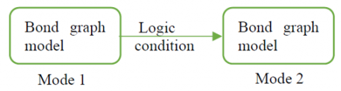
The simplest and the suitable kind of hybrid bond graph adapted to switched systems is the automaton coupling hybrid bond graph. It is a combination of bond graph and automaton [16]. It models the continuous dynamic by bond graph and the discrete transition through hybrid automaton [17]. Each different continuous evolution characterizes a mode, and a logic condition defines the transition from a mode to another as shown below in Figure 1.
Figure 1. Hybrid bond graph
The outputs/inputs are ordered by the flow/effort causality, which gives to bond graph the possibility to detect model errors and ensures a first layer of diagnosis.
Each bond graph element has a causality rule that organizes the effort and flow in the model. For a detailed review on this topic see [18, 19].
Inconsistencies of causality rules reveal modeling errors that have to be rectified before starting the diagnosis process.
2.2 Fault detection
Considering a switched system that evolves in n different modes and has m outputs. The state space represented in Eq. (1) gives the linear dynamic of a mode i $\in$ [1,n].
$S_{i}:\left\{\begin{array}{l}\dot{x}(t)=A_{i} \cdot x(t)+B_{i} \cdot u(t)+E_{i x} \cdot d(t) \\ y_{i}(t)=C_{i} \cdot x(t)+D_{i} \cdot u(t)+E_{i y} \cdot d(t)\end{array}\right.$ (1)
The method described in this paper is only concerned with sensor faults; therefore, $E_{i x}=0$ and the system is presented by Eq. (2).
$\mathrm{S}_{\mathrm{i}}:\left\{\begin{array}{c}\dot{\mathrm{x}}(\mathrm{t})=\mathrm{A}_{\mathrm{i}} \cdot \mathrm{x}(\mathrm{t})+\mathrm{B}_{\mathrm{i}} \cdot \mathrm{u}(\mathrm{t}) \\ y_{i}(t)=\mathrm{C}_{\mathrm{i}} \cdot \mathrm{x}(\mathrm{t})+\mathrm{D}_{\mathrm{i}} \cdot \mathrm{u}(\mathrm{t})+\mathrm{E}_{\mathrm{i}} \cdot \mathrm{d}(\mathrm{t})\end{array}\right.$ (2)
where, $x(t) \in \mathbb{R}^{k}$ is the state vector, $y(t) \in \mathbb{R}^{m}$ is the output vector, $u(t) \mathbb{R}^{p}$ is the input vector and $\mathrm{d}(\mathrm{t}) \mathbb{R}^{\mathrm{k}}$ is the defaults vector.
$A_{i} \in \mathbb{R}^{k * k}$ is the system matrix, $\mathrm{B}_{\mathrm{i}} \in \mathbb{R}^{\mathrm{k} * \mathrm{p}}$ is the control matrix, $C_{i} \in \mathbb{R}^{m * k}$ is the output matrix, $\mathrm{D}_{\mathrm{i}} \in \mathbb{R}^{\mathrm{m} * \mathrm{p}}$ is the feedthrough matrix and $\mathrm{E}_{\mathrm{i}} \in \mathbb{R}^{\mathrm{m} * \mathrm{k}}$ is the sensor defect matrix.
Each mode is described by Eq. (3).
$S_{i j}:\left\{\begin{array}{c}\dot{x}(t)=A_{i} \cdot x(t)+B_{i} \cdot u(t) \\ y_{i j}(t)=C_{i j} \cdot x(t)+D_{i j} \cdot u(t)+E_{i j} \cdot d(t)\end{array}\right.$ (3)
For each output j$\in$[1, m] evolving in a mode i$\in$ [1,n], we associate an observer. We have chosen Luenberger Observer for its simplicity and robustness and it can be represented by the mathematical Eq. (4).
$O_{i j}:\left\{\begin{array}{c}\check{\dot{x}}(t)=A_{i} \cdot \check{x}(t)+B_{i} \cdot u(t)+L_{i j}(y(t)-\check{y}(t)) \\ \check {y_{i j}}(t)=C_{i j} \cdot \check{x}(t)+D_{i j} \cdot u(t)\end{array}\right.$ (4)
$e_{i j}(t)$ in Eq. (5) is the calculated error between the rebuilt state $\check{x}(t)$ and the system state x (t).
$e_{i j}(t)=x(t)-\breve{x}(t)$ (5)
The residue $r_{i j}(t)$ in Eq. (6) is the calculated error between the rebuilt output $\check {y_{i j}}(t)$ and the measured output $y_{i j}(t)$.
$r_{i j}(t)=y_{i j}(t)-\check{y_{i j}}(t)$ (6)
Eq. (7) gives the derivative function of $r_{i j}(t)$ and $e_{i j}(t)$.
$\left\{\begin{array}{c}\dot{e}_{i j}(t)=\left(A_{i}-L_{i j} C_{i j}\right) \cdot e_{i j}(t)-L_{i j} E_{i j} d(t) \\ \dot{r}_{i j}(t)=C_{i j} \cdot e_{i}(t)+E_{i j} \cdot d(t)\end{array}\right.$ (7)
Observers receive all the outputs/ inputs of the system. Obtained outputs y(t) are compared instantly to rebuilt outputs $\check{y}$(t) to generate residual vectors rij.
Each residue $r_{i j}(t)$ calculated is compared to a dynamic threshold $m_{i j}$ (t), which is defined by Eq. (8).
$m_{i j}(t)=p_{i j}(t)+T_{i j}(t)$ (8)
Tij is a constant calculated by considering the noise measurements and the disturbances modeling errors in the system.
pij(t) is the observer's own error caused by the change of modes and calculation delays. It is the residue of observer when there is no default. It is defined by Eq. (11) resulting from Eq. (9) and Eq. (10).
$S_{i j}:\left\{\begin{aligned} \dot{x}(t)=& A_{i} \cdot x(t)+B_{i} \cdot u(t) \\ y_{i j}(t)=& C_{i j} \cdot x(t)+D_{i j} \cdot u(t) \\ & \mathrm{x}(0)=\mathrm{x}_{0} \end{aligned}\right.$ (9)
$O_{i j}:\left\{\begin{array}{c}\check{\dot{x}}(t)=A_{i} .\check{x}(t)+B_{i} \cdot u(t)+L_{i j}(y(t)-\check{y}(t)) \\ \check{y_{i j}}(t)=C_{i j} \cdot \check{x}(t)+D_{i j} \cdot u(t) \\ \check{x}(0)=\check{x}_{0}\end{array}\right.$ (10)
$p_{i j}(t)=y_{i j}(t)-\check{y_{i j}}(t)$ (11)
As a result, $m_{i j}$ is described by Eq. (12).
$m_{i j}(t)=y_{i j}(t)-\check{y_{i j}}(t)+T_{i j}$ (12)
We then adopt the decision logic bellow:
If ǀrij(t)ǀ> mij(t)
SCij =0 the output j is faulty
Else Sij=1
We then generate the sensors signature
SCj=$\prod_{i=1}^{n} S C i j$.
2.3 Mode identification
For an output $y_{j}$, the minimal value of the residue $r_{i j}(t)$ is the number of the active mode i.
Following the algorithm below, the residue $r_{i j}(t)$ will be evaluated to identify the corresponding mode of each output SMj:
for j=1:m
Min =$r_{i j}(t)$;
SMj = 1;
for j = 2:n
If $r_{i j}(t)$< Min
Min =$r_{i j}(t)$;
SMj = i;
end
end
end
SM=(SMj) $\in \mathbb{R}^{m}$
If the system functions normally with no errors, then SM(t)=C.U.
where, U is the unit vector, $U^{T}$ =$(11 \ldots 1)$, and C is the active mode.
Else, the $S M_{\mathrm{d}}(t)$ of the defected output is not identical to the others $S M_{\mathrm{j}}(t)$.
The active mode S is the mode of fault free outputs.
Supposing that we can't have all the sensors generating errors at the same time.
Then, $S=\frac{\sum_{j=1}^{m} S M_{j} * S C \mathrm{j}}{\sum_{j=1}^{m} S C \mathrm{j}}$.
Else, the active mode S is faulty.
3.1 System description
Figure 2 shows the two tanks system selected for the application of the fault detection and isolation approach.
We consider a two tanks hydraulic system. A pump delivers water at the rate q1 that arrives at a first tank T1 of section S1. At the exit of this tank a valve V1 of hydraulic resistance Rh lets the fluid passes to a second tank T2, of section S2. Thus, the outflow from this tank is allowed by a valve V2 of hydraulic resistance Rh.
In order to facilitate the study, the valve V1 is left open and only the valve V2 is acted on.
We can have two states of the valve V2: closed or opened.
In mode 1, V2 is closed and q1 is maintained.
In mode 2, V2 is opened and q1 is stopped.
The aim is to maintain the liquid level l1 and l2 in the two tanks T1 and T2 on a well-defined level: $\left\{\begin{array}{l}l 1 \leq 0.6 \\ l 2 \geq 0.2\end{array}\right.$.
Table 1 presents the numerical values of parameters.
Figure 2. Two tanks hydraulic system
Table 1. Parameters numerical values
|
Parameter |
Description |
Value |
|
q1 |
volumetric flow rate |
0.2 $\mathrm{m}^{3} / \mathrm{s}$ |
|
Rh |
Hydraulic resistance of the valve |
10 N.s.m $^{-5}$ |
|
S1 |
Base surface area of the tank1 |
2 $m^{2}$ |
|
S2 |
Base surface area of the tank2 |
1.5 $m^{2}$ |
|
g |
gravitational acceleration |
$9.8 m . s^{-2}$ |
The hybrid automaton in Figure 3 presents the different standard states of the system described by mode 1 and mode 2. Satisfying the conditions allows jumping from a mode to another.
Figure 3. Hybrid automaton of the system
3.2 System modeling
To build a bond graph model in integral causality, the following suppositions are taking into account:
-The volumetric flow rate q is the volume of fluid which passes per time; it is defined by Eq. (13).
$q=\frac{d V}{d t}$ (13)
-The volumetric flow rate q1 of the pump is constant.
-The hydraulic resistance Rh is the resistance resulting from a liquid flowing valves or changes in pipe diameter; it is defined by Eq. (14).
$R=\frac{Q}{\Delta P}$ (14)
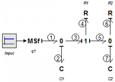
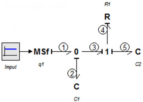
Figure 4 and Figure 5 present the bond graph model in integral causality.
A bond graph model is designed for each mode:
Second mode :
Figure 4. Bond graph model: mode 2
First mode:
Figure 5. Bond graph model: mode 1
To generate the dynamic model of the system we follow the four steps below:
- Identify the outputs/inputs variables.
- Extract equations from junctions.
- Extract equations from passive and active elements.
- Combine the set of equations to generate the state space.
The equations Eq. (15), Eq. (16), Eq. (17), Eq. (24) and Eq. (25) extracted from the junctions “0” and “1,” of the BG model are presented for the two modes below:
Second mode:
$\left\{\begin{array}{c}e 1=e 2=e 3=\{h 1\} \\ f 1=f 2+f 3\end{array}\right.$ (15)
$\left\{\begin{array}{l}f 3=f 4=\mathrm{f} 5 \\ e 3=e 4+e 5\end{array}\right.$ (16)
$\left\{\begin{array}{c}e 5=e 6=e 7=\{h 2\} \\ f 5=f 6+f 7\end{array}\right.$ (17)
The constitutive equations in Eq. (18) of the BG elements are presented below:
$e 4=R 1 \cdot f 4 ; e 6=R 2 \cdot f 6 ; f 7=C 2 \cdot \frac{d e 7}{d t} ;$
$f 2=C 1 \cdot \frac{d e 2}{d t} ; R 1=R 2=\frac{R H}{g} ; C 1=S 1 ; C 2=S 2$ (18)
The system dynamic model can be described in the form below in Eq. (19):
$\left\{\begin{array}{c}\frac{d l 1}{d t}=\frac{q 1}{s 1}+\frac{g}{R H * S 1}(l 2-l 1) \\ \frac{d l 2}{d t}=\frac{g}{R H * S 2}(l 1-l 2)-\frac{g}{R H * S 2} l 2\end{array}\right.$ (19)
The system can be represented under the state space equations below in Eq. (20):
$\left\{\begin{array}{c}\dot{X}=A_{2} \cdot X+B_{2} \cdot u \\ Y=C_{2} \cdot X\end{array}\right.$ (20)
where, X=$\left(\begin{array}{l}e 2 \\ e 7\end{array}\right)$ =$\left(\begin{array}{l}l 1 \\ l 2\end{array}\right)$.
Eq. (21) represents the system matrix.
$A_{2}=\left(\begin{array}{cc}-\frac{g}{R H * S 1} & \frac{g}{R H * S 1} \\ \frac{g}{R H * S 2} & -\frac{2 g}{R H * S 2}\end{array}\right)$ (21)
Eq. (22) represents the control matrix.
$B_{2}=\left(\begin{array}{l}0 \\ 0\end{array}\right)$ (22)
Eq. (23) represents the output matrix.
$C_{2}=\left(\begin{array}{ll}1 & 0 \\ 0 & 1\end{array}\right)$ (23)
First mode:
$\left\{\begin{array}{c}e 1=e 2=e 3=\{h 1\} \\ f 1=f 2+f 3\end{array}\right.$ (24)
$\left\{\begin{array}{l}f 3=f 4=\mathrm{f} 5 \\ e 3=e 4+e 5\end{array}\right.$ (25)
Eq. (26) gives the constitutive equations of the BG elements:
$e 4=R 1 \cdot f 4 ; f 2=C 1 \cdot \frac{d e 2}{d t} ; f 5=C 2 \cdot \frac{d e 5}{d t}$;
$R 1=R 2=\frac{R H}{g} ; C 1=S 1 ; C 2=S 2$ (26)
The system dynamic model can be described in the form below in Eq. (27).
$\left\{\begin{array}{l}\frac{d l 1}{d t}=\frac{q 1}{s 1}+\frac{g}{R H * S 1}(l 2-l 1) \\ \frac{d l 2}{d t}=\frac{g}{R H * S 2} l 1-\frac{g}{R H * S 2} l 2\end{array}\right.$ (27)
The system can be represented under the state space equations below in Eq. (28).
$\left\{\begin{array}{c}\dot{X}=A_{1} \cdot X+B_{1} \cdot u \\ Y=C_{1} \cdot X\end{array}\right.$ (28)
where, X=$\left(\begin{array}{c}e 2 \\ e 5\end{array}\right)$ =$\left(\begin{array}{l}l 1 \\ l 2\end{array}\right)$.
Eq. (29) represents the system matrix.
$A_{1}=\left(\begin{array}{cc}-\frac{g}{R H * S 1} & \frac{g}{R H * S 1} \\ \frac{g}{R H * S 2} & -\frac{2 g}{R H * S 2}\end{array}\right)$ (29)
Eq. (30) represents the control matrix.
$B_{1}=\left(\begin{array}{l}0 \\ 0\end{array}\right)$ (30)
Eq. (31) represents the output matrix.
$C_{1}=\left(\begin{array}{ll}1 & 0 \\ 0 & 1\end{array}\right)$ (31)
3.3 Observer-based fault diagnosis
To applicate our method, we have chosen Luenberger Observer for its simplicity and robustness. Eq. (32) describes its mathematical model.
$O_{i j}:\left\{\begin{array}{c}\check{\dot{x}}(t)=A_{i} \cdot \breve{x}(t)+B_{i} \cdot u(t)+L_{i j}(y(t)-\breve{y}(t)) \\ \breve{y}_{j}(t)=C_{i j} . \check{x}(t)+D_{i j} \cdot u(t) \\ \check{x}(0)=\check{x}_{0}\end{array}\right.$ (32)
In this example, we have a set of four observers: $O_{i j}$, i $\in$ {1, 2}, j $\in$ {1, 2}. Each output is linked to an observer.
To calculate the observer gains we have used the technique of pole placement, and the poles are selected as follows in Eq. (33).
$P_{11}=P_{12}=P_{21}=P_{22}=\left(\begin{array}{l}-40+i \\ -40-i\end{array}\right)$ (33)
The observers gains are then calculated in Eq. (34).
$L_{11}=10^{2}\left(\begin{array}{c}0.789 \\ 31.622\end{array}\right) ; L_{12}=10^{2}\left(\begin{array}{c}23.914 \\ 0.789\end{array}\right)$
$L_{21}=10^{2}\left(\begin{array}{c}0.782 \\ 30.582\end{array}\right) ; L_{22}=10^{2}\left(\begin{array}{c}23.914 \\ 0.782\end{array}\right)$ (34)
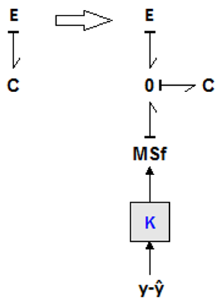
The design of a BG model corresponding to the observer equations is the next step, and the OBG is constructed by adding the term $L(Y-\check{Y})$ to the bond graph model.
In Figure 6, the integration of the term $L(Y-\check{Y})$ into the dynamic element C, using the modulated effort source MSe, is made. The idea is to have a BG model corresponding to the observer equation in Eq. (32).
The symbol “E” represents a BG element to which C is linked.
Figure 6. Element C equivalent
Second mode:
Figure 7. Bond graph model: observer 2
First mode:
Figure 8. Bond graph model: observer 1
Figure 7 and Figure 8 represent respectively the observer bond graph model of mode 2 and mode1.
The components of the vector $L_{i j}$, i $\in$ {1, 2}, j $\in$ {1, 2} are represented by K1 and K2.
3.4 Simulation results
To have reliable results, the system has been simulated using the following two powerful software: 20-sim and Matlab.
Figure 9 represents the normal evolution of the continuous and the discrete states. When the conditions are satisfied the system jumps from a mode to another. In order to simulate the system in all modes the simulation time is fixed at 20s.
We can observe that each mode is distinguished by its proper evolution and the water variation level in the two tanks doesn’t exceed the preliminary defined thresholds.
Figure 9. The hybrid evolution of parameters
The proposed method in this article should be tested to prove its efficiency. Thus, we will add a sensor fault and show the response of the system, which should be able to detect the fault and locate the active mode.
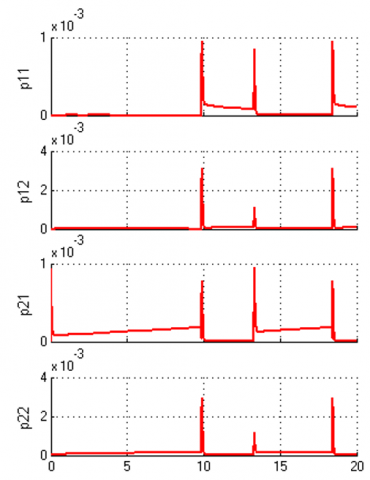
The fault detection approach compares the calculated residues to a defined thresholds mij(t) which is the sum of pij(t) and Tij.
Figure 10 shows the evolution of Pij(t) which are the residues of the faultless system. We observe clearly that they are not equal to zero and observers have their own errors which will be eliminated using our method.
The constant Tij chosen is given below:
$T_{11}=T_{12}=T_{21}=T_{22}=5.10^{-4}$
Figure 11 presents the sensors signature based on the result of the residues evaluation.
Sensors signatures have identified the default, and the detection of the active mode will be the next step.
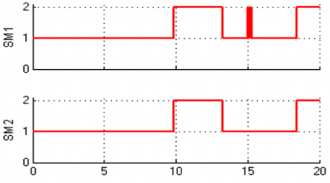
The modes signatures of each output are represented in Figure 12.
Based on modes signatures, the proposed algorithm locates the active mode, and a comparison between the estimation and the real modes is represented in Figure 13.
We observe clearly that the estimated and the real modes are identical.
Figure 10. Residues
Figure 11. Sensors signature
Figure 12. Mode’s signature
Figure 13. Real modes VS estimated modes
Applying the proposed approach on the above example has shown its efficiency and reliability to detect and locate faults.
Thanks to the easy application of our diagnosis algorithm, it can be deployed and implemented in industry.
In this paper, we have discussed fault detection and isolation problem for switched systems, and we have proposed a solution consisting of three steps.
In the first step, the bond graph is used to model the system, and the hybrid automaton takes into account the transition between modes to allow modeling of the two continuous and discrete parts of the switching systems.
After modeling, the next step is the generation of residues ensured by observers. The bond graph is also used in this step to ensure the detection of modeling faults.
The last step aims to cancel the observer's error and analyze the residues to detect faults and locate the active mode.
Most studies have focused on diagnosis schemes, system modeling, and residual generation. However, they have neglected the importance of thresholds, which play a crucial role in making fault existence decisions. Achieving a high level of precision is only possible through dynamic thresholds. Thus, we have proposed a new diagnosis approach using dynamical thresholds. The main gain of this technique is its powerful potential to detect sensor faults and avoid false alarms.
This paper has discussed sensor faults. However, the extension of the proposed approach to actuator faults is a pertinent standpoint to broaden the method and make it more efficient.
[1] Chiang, L.H., Russell, E.L., Braatz, R.D. (2000). Fault Detection and Diagnosis in Industrial Systems. Springer Science & Business Media.
[2] Venkatasubramanian, V., Rengaswamy, R., Kavuri, S.N., Yin, K. (2003). A review of process fault detection and diagnosis: Part III: Process history based methods. Comput. Chem. Eng., 27(3): 327‑346. https://doi.org/10.1016/S0098-1354(02)00162-X
[3] Bachir, S., Tnani, S., Trigeassou, J.C., Champenois, G. (2006). Diagnosis by parameter estimation of stator and rotor faults occurring in induction machines. IEEE Trans. Ind. Electron., 53(3): 963‑973. https://doi.org/10.1109/TIE.2006.874258
[4] Patton, R.J., Chen, J. (1991). A review of parity space approaches to fault diagnosis. IFAC Proc., 24(6): 65‑81. https://doi.org/10.1016/S1474-6670(17)51124-6
[5] Hammouri, H., Kinnaert, M., El Yaagoubi, E.H. (1999). Observer-based approach to fault detection and isolation for nonlinear systems. IEEE Trans. Autom. Control, 44(10): 1879‑1884. https://doi.org/10.1109/9.793728
[6] Abboudi, A., Belmajdoub, F. (2020). A new diagnosis approach of hybrid systems through observers and hybrid automata. Int. J. Autom. Smart Technol., 10(1): 135‑143.
[7] Doraiswami, R., Cheded, L. (2017). Fault Detection and Isolation, Fault Diagnosis and Detection, Mustafa Demetgul and Muhammet Ünal, IntechOpen, 2017. https://doi.org/10.5772/67870
[8] Borutzky, W. (2011). Bond Graph Modelling of Engineering Systems: Theory, Applications and Software Support. New York: Springer-Verlag. https://doi.org/10.1007/978-1-4419-9368-7
[9] Liberzon, D. (2005). Switched Systems. in Handbook of Networked and Embedded Control Systems, D. Hristu-Varsakelis et W. S. Levine, Éd. Boston, MA: Birkhäuser, 559‑574. https://doi.org/10.1007/0-8176-4404-0_24
[10] Mahmoud, M.S. (2010). Switched Systems. in Switched Time-Delay Systems. In: Switched Time-Delay Systems. Springer, Boston, MA. https://doi.org/10.1007/978-1-4419-6394-9_4
[11] Abboudi, A., Belmajdoub, F. (2021). Hybrid diagnosis method applied to switched mechatronic systems. Journal Européen des Systèmes Automatisés, 54(5): 683‑691. https://doi.org/10.18280/jesa.540503
[12] Rosenberg, R.C., Karnopp, D.C. (1972). A definition of the bond graph language. J. Dyn. Syst. Meas. Control, 94(3): 179‑182. https://doi.org/10.1115/1.3426586
[13] Low, C.B., Wang, D., Arogeti, S., Zhang, J.B. (2009). Causality assignment and model approximation for hybrid bond graph: Fault diagnosis perspectives. IEEE Trans. Autom. Sci. Eng., 7(3): 570‑580. https://doi.org/10.1109/TASE.2009.2026731
[14] Roychoudhury, I., Daigle, M.J., Biswas, G., Koutsoukos, X. (2011). Efficient simulation of hybrid systems: A hybrid bond graph approach. Simulation, 87(6): 467‑498. https://doi.org/10.1177%2F0037549710364478
[15] Mosterman, P.J. (1997). Hybrid Dynamic Systems: A hybrid bond graph modeling paradigm and its application in diagnosis. Vanderbilt University, 1997.
[16] Ezzahra, O.F., Zanzouri, N. (2016). Hybrid dynamical system monitoring based on bond graph. Proceedings of Engineering & Technology, 332-337.
[17] Kohavi, Z., Jha, N.K. (2009). Switching and Finite Automata Theory. Cambridge University Press.
[18] Bond Graph Causality Assignment and Evolutionary Multi-Objective Optimization | SpringerLink. https://link.springer.com/chapter/10.1007%2F978-1-4020-6264-3_75.
[19] Borutzky, W. (2010). Analysis of causal bond graph models. in Bond Graph Methodology: Development and Analysis of Multidisciplinary Dynamic System Models, London: Springer, 223‑303. https://doi.org/10.1007/978-1-84882-882-7_6