Amir Majid
© 2021 IIETA. This article is published by IIETA and is licensed under the CC BY 4.0 license (http://creativecommons.org/licenses/by/4.0/).
OPEN ACCESS
The aim of this work is to evaluate the nth joined probability of three-dimensional wireless sensor networks, and to extend the lifetime of these networks. A Gaussian probability distribution function is assumed for the power coverage probability for each sensor in the 3-dimensional cartesian and spherical coordinates. The overall joint probability is evaluated from each sensor to a target in the network, and then the network lifetime of sensors power sensing a number of targets, is extended based on removing redundancies of powering all sensors at the same time. Proportional to the evaluated probabilities, sensors are energized during slots of periodic time. The formulated probabilities are assumed to be uncorrelated among each sensor to any target zone. A case study is introduced to demonstrate extending the lifetime of a network comprising 7 sensors targeting two uncorrelated zones, in which 8 different cases of subsets are formed, when a minimum threshold of overall power coverage probability of 35% is assumed. Network lifetime is extended more than 70%, with some sensors reaching more than 90% power saving. This work can be extended to deal with other types of probabilities, as well as with cases of correlated sensor-target coverages.
power coverage, Gaussian, joint probability, sensor lifetime, wireless network networks
Wireless sensor networks (WSN) are widely used nowadays to sense numerous domestic and industrial applications remotely, without much of human intervenes. Some of these applications are listed in the literature, such as multi-channel data collection capacities [1, 2], mobile and broadcasting ad hoc networks [3, 4], coverage with multiple sensors [5], multi-regional query scheduling of wireless networks [6], and many other applications. An earlier concise survey of wireless networks can be found in Akyildiz et al. [7]. Whilst such wireless network advantages are readily obvious, they suffer from the shortcoming of power supply, since it is mainly por+ with limited capacities, that leads to shortening the lifetime of such sensor networks infrastructures. Other disadvantages can also exist, such as sensing range, storage capabilities, and computational limitations.
The scope of most of the work conducted on WSN, is to evaluate power coverage probabilities of the sensor networks and extend their lifetimes, by removing redundancies from powering the entire network sensors at the same time, instead of allowing some groups of sensors to operate at one time. Several studies examined this general case with several two dimensional planner network algorithms, such as the construction of a decentralized tree for data aggregation [8], using shortest path aggregation tree [9], and data collection with wireless networks aggregation [10], yet in this work, we use the concept of deterministic network model (DNM), in which pairing of sensors occur if their physical distances are within the transmission radius, otherwise disconnected, as depicted in a reference book [11]. The reference [12] deals with preserving target coverage using computational geometry, whereas [13] deals with distributed active sensors selecting scheme, the two forthcoming fields of which, might be similar with this paper, yet ours is in three-dimension. The physical distance here, is the power coverage distance, that relies on the individual sensor probabilities covering one or more targets.
Although there were many empirical studies that employ this deterministic model concept, such as analyzing transitional regions of wireless networks [14], and WSN controlling topologies [15], we implement here third-dimensional joint probabilities, based on the Gaussian probability density (PDF). To increase the network lifetime, sensors are grouped in subsets, such that individual subsets cover several targets at a time, hence eliminating redundancies of powering all sensors at the same time. With this arrangement, the portable power supply can be spared for longer times. This concept has been employed in other methods, such as greedy based [16], genetic [17], linear programming and optimization [18], and heuristic greedy optimum algorithm [19], all of which deal with scheduling schemes and other probabilistic analyses. Scenarios of sensor-target coverage cases were studied [20], dealing with load demand switching, sensors position layouts and perturbations in load and position, in which all these studies, are based on the α-Reliable Maximum Sensor Coverage (α-RMSC) problem. We assume that the network is smart in switching sensors on/off as required to eliminate redundancies and as a result extending network lifetime.
To the author knowledge, there were no dominate work on three-dimensional WSN. With 3rd-dimensional arrangement, the problem of coverage probabilities become unpredictable due to the correlation of probability in three coordinates, whether cartesian or spherical coordination, as well as the correlation of each sensor with the next, in covering individual target zones. The analysis of these cases is conducted in this study, with the aim of extending the entire network lifetime, using a certain probability density function. Whilst there exist several types of probability density functions, we assume only a normal (Gaussian) PDF of power coverage among all sensors and in each of the three space coordinates. We shall consider power coverage to be the random variable for the Gaussian PDF.
The aim of this work is not to solely determine probabilities, but to extend network lifetime by evaluating and comparing joint probabilities of groups of sensors covering targets, in order to remove redundancies. In this context, it is assumed that there exists an option to control sensors by varying their power supply, by switching sensors on/off, and by varying the time of energizing sensors. This requires thee WSN to be a smart network.
We shall assume that power coverage probability from any sensor to target, as a single random variable with respect of distance x, is Gaussian in nature, as:
$f_{X}(x)=\frac{1}{\sqrt{2 \pi \sigma^{2}}} \exp \left(-\frac{(x-m)^{2}}{2 \sigma^{2}}\right)$ (1)
where, $\sigma$ is variance, and $m$ is the mean. This function can be generalized to be the joint Gaussian PDF for a vector of $\mathrm{N}$ random variables, with mean vector $\boldsymbol{\mu}_{x}$ and covariance vector $\boldsymbol{C}_{X X}$, as:
$f_{X}(x)=\frac{1}{\sqrt{(2 \pi)^{N} \operatorname{det}\left(\boldsymbol{C}_{X X}\right)}} e^{\left\{-0.5\left(x-\mu_{x}\right)^{T} C_{X X}^{-1}\left(x-\mu_{X}\right)\right\}}$ (2)
with correlation factors $\rho_{i j}$ between sensors $\mathrm{i}$ and $\mathrm{j}$, that's the off-diagonal elements are $\rho_{i j} \sigma_{i} \sigma_{j}$, whereas the diagonal elements are $\sigma_{i}^{2}, i=1, N$. With uncorrelated case, the offdiagonal elements are all zero, hence $\boldsymbol{C}_{X X}=\left[\begin{array}{l}\left.\sigma_{1}^{2} \sigma_{2}^{2} \sigma_{3}^{2} . .\right] \text { ] }\end{array}\right.$ One can deduce that the joint probability of three uncorrelated random variables in cartesian coordinates $v_{i=1,3}=[x, y, z]$, is $f_{X, Y, Z}(x, y, z)$, that's
$f_{V}(v)=\prod_{n=1}^{N} \frac{1}{\sqrt{2 \pi \sigma_{n}^{2}}} e^{\left\{-\frac{\left(v_{n}-\mu_{n}\right)^{2}}{2 \sigma_{n}^{2}}\right\}}$ (3)
It might be appropriate sometimes to transfer the joint Gaussian probability from the cartesian coordinates to the spherical coordinates, since each sensor can be visualized as spheres with coordinates $[r, \theta, \emptyset]$, since $r=\sqrt{x^{2}+y^{2}+z^{2}}$, $\emptyset=\tan ^{-1}\left(\frac{y}{x}\right), \theta=\cos ^{-1}\left(\frac{z}{r}\right)$, yet the inverse transformation is maybe more appropriate, i.e., $x=r \sin (\theta) \cos (\emptyset), y=$ $r \sin (\theta) \sin (\emptyset, z=r \cos (\theta)$.
$f_{R, \Theta, \Phi}(r, \theta . \emptyset)=f_{X, Y, Z}(x, y, z) a b s\left\{\operatorname{det}\left[J\left(\begin{array}{lll}x & y & Z \\ r & \theta & \varnothing\end{array}\right)\right]\right\}$ (4)
where, J is the Jacobian operator, in which $J\left(\begin{array}{lll}x & y & z \\ r & \theta & \emptyset\end{array}\right)$ is equal to:
$\left[\begin{array}{ccc}\sin (\theta) \cos (\emptyset) & \sin (\theta) \sin (\emptyset) & \cos (\theta) \\ r \cos (\theta) \cos (\emptyset) & r \cos (\theta) \sin (\emptyset) & -r \sin (\theta) \\ -r \sin (\theta) \sin (\emptyset) & r \sin (\theta) \cos (\emptyset) & 0\end{array}\right]$ (5)
and $\operatorname{det}\left\{J\left(\begin{array}{lll}x & y & z \\ r & \theta & \emptyset\end{array}\right)\right\}=r^{2} \sin (\theta) .$ Simplifying the above equation with substituting $x, y$ and $z$ values, yields,
$f_{R, \Theta, \Phi}(r, \theta . \emptyset)=\frac{r^{2} \sin (\theta)}{\left(2 \pi \sigma^{2}\right)^{3 / 2}} \exp \left(-\frac{r^{2}}{2 \sigma^{2}}\right)$ (6)
Next, we shall evaluate the joint power coverage probability in three-dimensional space for all sensors acting on one target zone, and later on, we extend this concept to multiple uncorrelated target zones, hence, evaluating the total probability of the entire wireless sensor network.
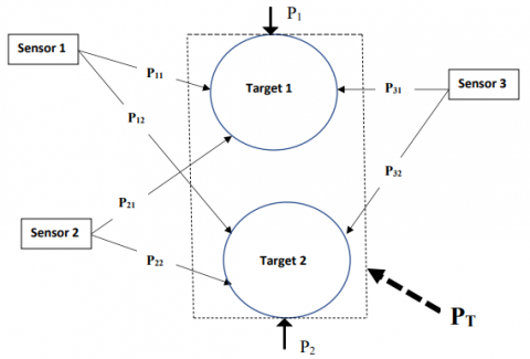
To extend network lifetime, the redundancies of powering sensors should be eliminated, based on their coverage probabilities. Let’s consider a section of the network, where three sensors acting on two target zones, as depicted in Figure 1.
Figure 1. Wireless sensor network with three sensors covering two target zones
First, we shall assume that the sensor coverage probabilities lower than a certain minimum threshold value, are excluded. This would help to control the reliability of forthcoming evaluations. As a result, sensors are grouped into subsets that act on any single target, with their nth joint probabilities, evaluated in three-dimensional spherical coordination. For simplicity, the probabilities whether in the (r, θ, Ø) spherical coordinates or (x, y, z) cartesian coordinates, are considered to be uncorrelated.
The selection of sensor groups is not straightaway, as there can be in general as many as 2N-1 subsets for any N number of sensors. This would impose computational limitation on the method used here, since the joint probability of each subset has to be calculated to eliminate redundancies by eliminating subsets according to their probabilities. In this context, the joint probability is calculated according to the following algorithm:
$F_{i j}=1-P_{i j}$ (7)
where, $P_{i j}$ is the coverage probability from sensor $i,(i=1, N$ sensors) to target $j(j=1, M$ targets $)$, and $F_{i j}$ is the power failure probability. The joint probability on any target is then,
$P_{j}=1-\prod_{i=1}^{N} F_{i j}$ (8)
where, $P_{j}$ is the joint probability of $n$ sensors on target $j$. To find the entire network probability $P_{T}$ of all target zones, we assume that the joint probabilities of sensor subsets on any target zone are independent and uncorrelation among them, i.e.
$P_{T}=\prod_{j=1}^{M} P_{j}$ (9)
Powering sensor subsets, and sensors within any subset, are based on their calculated joint probabilities in a linear proportionality. In this context, the periodic time of powering sensors, is divided into slots in which each subset of sensors, is activated at a time depending on the joint probability. Further, each sensor within a subset is powered during a time that is proportional with the individual sensor-target probability. It is assumed that this network is smart to be able to switch on/off individual sensors as required.
A simulation of a wireless sensor network of 7 sensors covering two target zones, is simulated. We assume a base case of 1st order probability of the coverage power within a range of unit distance x, to be Gaussian in nature, with mean variance values of unity. Other realistic values based on practical implementations, can also be used with the similar effect of eliminating redundancies, with reference to the standard case.
4.1 Three-dimensional sensor network
To extend power coverage probability to three-dimensional space environment, similar values of the mean of the joint Gaussian probability density function in each coordinate of the cartesian coordinates; x, y and z, are assumed. The same assumption is applied for the variances. Therefore, in this case maximum probability of 100% is assumed to be at the origin of $x=y=z=1$, with reference to Eq. (3),
$f_{X, Y, Z}(x, y, z)=f_{V}(v)=\prod_{n=1}^{3} \frac{1}{\sqrt{2 \pi \sigma_{n}^{2}}} e^{\left\{-\frac{\left(v_{n}-\mu_{n}\right)^{2}}{2 \sigma_{n}^{2}}\right\}}$ (10)
hence, $f_{V}(v)=f_{X, Y, Z}(x, y, z)=\frac{1}{(2 \pi)^{1.5} e}$.
This value is computed as $0.063493=6.3493 \%$ and used as a reference with 100% probability. Other coordinate values of x,y,z are referenced to this. Hence, the referenced probabilities of the 7 sensors with the following coordinates, are calculated as,
The Table 1 depicts power coverage probabilities due to sensors allocated at the above different coordinates, alternatively, any sensor allocated at the origin, would cover distances equal to the above coordinates, with same probabilities.
Table 1. Third-dimensional coverage probabilities for cartesian coordinates
|
Sensor |
x |
y |
z |
Probability fX,Y,Z(x,y,z) |
Sensor Power sharing |
|
1 |
1 |
0 |
0 |
2.330 % |
9.36% |
|
2 |
0 |
1 |
0 |
2.330 % |
9.36% |
|
3 |
0 |
0 |
1 |
2.330 % |
9.36% |
|
4 |
1 |
1 |
0 |
3.851% |
15.47% |
|
5 |
1 |
0 |
1 |
3.851% |
15.47% |
|
6 |
0 |
1 |
1 |
3.851% |
15.47% |
|
7 |
1 |
1 |
1 |
6.349% |
25.47% |
Notes: The joint probability fX,Y,Z(x,y,z) is for the random variables {x,y,z}, with each sensor sharing of the coverage power, as a percentage.
4.2 Transforming to spherical coordinates
To transfer from Cartesian to spherical coordinates using, $x=r \sin (\theta) \cos (\emptyset), y=r \sin (\theta) \sin (\emptyset), z=r \cos (\emptyset)$, as well as, $\operatorname{det}\left[J\left(\begin{array}{lll}x & y & Z \\ r & \theta & \emptyset\end{array}\right)\right]=r^{2} \sin (\theta)$, and applying the case of 7 sensors, yields the following Table 2.
Table 2. Third-dimensional coverage probabilities for spherical coordinates
|
Sensor |
x,y,z |
r |
θ |
Probability fR,Θ,Φ(r,θ,Ø) |
Referenced probability |
|
1 |
1,0,0 |
1 |
900 |
2.330% |
14.98 % |
|
2 |
0,1,0 |
1 |
900 |
2.330% |
14.98 % |
|
3 |
0,0,1 |
1 |
900 |
2.330% |
14.98 % |
|
4 |
1,1,0 |
1.414 |
900 |
7.702% |
49.52% |
|
5 |
1,0,1 |
1.414 |
450 |
5.445% |
35.01% |
|
6 |
0,1,1 |
1.414 |
450 |
5.445% |
35.01% |
|
7 |
1,1,1 |
1.732 |
550 |
15.551% |
100% |
Notes: The joint probability with cartesian coordinates, are transferred to spherical coordinates. These probabilities are referred on the seventh sensor.
The above table presents power coverage probabilities in third-dimensional spherical coordinates, which can be suitable in some cases for determining the joint properties of several sensors with no correlation among them.
4.3 Sensor joint probabilities formulation
To evaluate the joint Gaussian probability of the power range of sensors covering one target zone, we implement Eq. (6) and (7) for the 7 sensors. We shall employ the spherical coordinates in this respect, with the assumption that there are no correlations among sensor probabilities.
As stated earlier, there are 2N-1 subsets for N sensors, that must be considered to eliminate redundancies. This might impose computational difficulties, yet, the majority of these cases are omitted due to lack of entire coverage probability to be more than a threshold value. This limit value is determined by the user. In our case, let’s define a minimum probability threshold value of say 30-35%.
It may be possible to find an algorithm that computes the necessary number and coordinates of sensors to achieve the minimum probability threshold, although this has not been applied. yet a logical estimation of these possibilities can be made. For instance, we shall omit the case of installing several sensors in the same place, as this imply changing the mean and covariance values set earlier for this example. Also, it is needed to install more sensors to achieve this conditional probability, since sensor 7 that has highest probability, will not be able to provide a probability larger than 25.47% alone. Further, it is needed at least sensors, 7,6,5 & 4 to achieve this, as together a coverage probability of approximately 30% is achieved.
Hence, there are only 8 cases, as depicted in the following Table 3. For each case, subset, subset members and subset probability are shown, together with subset time sharing. There are 8 different activation slots in a time period, for each case, that are proportional with their probabilities.
Table 3. Coverage probabilities and activation times for 8 sensor subsets
|
Subset |
Sensor Subset |
Coverage Probability |
Activation Time Slot |
|
1 |
{7-6-5-4-3-2-1} |
35% |
13.4% |
|
2 |
{7-6-5-4-3-2} |
33.5% |
12.8% |
|
3 |
{7-6-5-4-2-1} |
33.5% |
12.8% |
|
4 |
{7-6-5-3-2-1} |
33.5% |
12.8% |
|
5 |
{7-6-5-4-1} |
32% |
12.2% |
|
6 |
{7-6-5-3-1} |
32% |
12.2% |
|
7 |
{7-6-5-2-1} |
32% |
12.2% |
|
8 |
{7-6-5-1} |
30% |
11.5% |
Notes: The joint probability for each subset group are displayed as percentages with proportional activation during time slots as percentages.
4.4 Lifetime extension method
To evaluate the extension of sensor network lifetime for the 8 subsets, each with different number and different locations of sensors, Table 4 depicts power sharing percentage of each sensor in a subset, as well power sharing percentage of subset during time slots in a periodic switching time. It can be seen from the above table that the wireless sensor network for this case study can be extended 72% minimum, since further power savings on other sensors can be increased up 93.6%. All figures in table are rounded. It can be noticed that this method requires computational routine to evaluate the so many subsets for large number of network sensors. This is not within this work scope. Further, we have assumed that sensor switching on/off during activation timings, is possible, such as smart networks.
Table 4. Power sharing of 8 subsets of sensors, with each containing a maximum of 7 sensors
|
SS |
S1 |
S2 |
S3 |
S4 |
S5 |
S6 |
S7 |
|
1 |
12% .016 |
12% .016 |
12% .016 |
17% .021 |
17% .021 |
17% .021 |
28% .035 |
|
2 |
12% .016 |
off |
12% .016 |
17% .021 |
17% .021 |
17% .021 |
28% 0.035 |
|
3 |
12% .016 |
12% .016 |
off |
17% .021 |
17% .021 |
17% .021 |
28% .035 |
|
4 |
off |
12% .016 |
12% .016 |
17% .021 |
17% .021 |
17% .021 |
28% .035 |
|
5 |
12% .016 |
off |
off |
17% .021 |
17% .021 |
17% .021 |
28% .035 |
|
6 |
off |
12% .016 |
off |
17% .021 |
17% .021 |
17% .021 |
28% .035 |
|
7 |
off |
off |
12% .016 |
17% .021 |
17% .021 |
17% .021 |
28% .035 |
|
8 |
off |
off |
off |
17% .021 |
17% .021 |
17% .021 |
28% .035 |
Notes: SS stands for sensor subset. Each subset row indicates sharing percentages of each sensor in the subset time slot of activation, as well as coverage probability values.
Note that for the above table, each sensor cell is divided into two information, namely the percentage of time sharing of energizing the sensor referenced within the allotted subset timing, and underneath is the absolute sensor power sharing. This can be summarized as,
|
Share |
0.064 |
0.064 |
0.064 |
0.168 |
0.168 |
0.168 |
0.28 |
|
Save |
93.6 |
93.6 |
93.6 |
83.2 |
83.2 |
83.2 |
72 |
Notes: The first row shows the seven sensors power sharing, whereas the second row indicates the percentage of power saving for each sensor.
Figure 2 [20], depicts the different methods of sensors power sharing within the subsets, that’s fixed subset - fixed sensor timings, variable subset - fixed sensors, fixed subsets - variable sensors and variable subsets - variable sensor timings. The later was implemented in the case study, yet any method can be implemented. It can be noticed from Table 4, that subset timing doesn’t change much compared to the ideal case of 12.5%, whereas sensor timing has substantial effect of removing redundancies.
Figure 2. Different methods of removing power sharing redundancies
4.5 Multiple targets formulation
To extend the method of determing the joint coverage probability of all sensors on several targets, we have to recognize if there were correlations among the different targets coverages by the same sensors. Correlation can be determined from experimental data of sensors coverage.
4.5.1 Uncorrelated target coverage
In this case, we shall keep the same network configuration but with replacing the coordinates of targets with sensors in our case example, i.e. there are one sensor at (0,0,0) covering 7 targets {(0,0,1),(0,1,0),(0,1,1),(1,0,0),(1,0,1),(1,1,0)(1,1,1)}, Hence, using Table 1, we deduce that there will be no joint probability as, $P_{T}=(9.36 \%)^{3}(15.47 \%)^{3}(25.47 \%) \sim 0 \%$. Yet any number of n sensors covering m targets, can be analyzed by using Eqns. (7), (8) & (9), with the assumption that there are no correlations of power covering among all target zones, which means that the joint probability of all sensors towards one target is independent of the same sensors’ coverage on other targets. For example, if a second target is placed at (0,0,0), and knowing that there is a 30-35% minimum threshold coverage value, then $P_{T}=P_{1} P_{2}=10 \%$, where $P_{1}$ and $P_{2}$ are the power coverages of all sensors on target 1 and 2 , respectively.
4.5.2 Correlated target coverage
In this case, let’s assume that there are the same 7 sensors, covering two correlated targets. This time the sensors are at: {(0,0,1),(0,1,0),(0,1,1),(1,0,0),(1,0,1),(1,1,0)(0,0,0)}, whereas the targets are at target 1=(0.5,1,0.5) and target 2 = (1,0.5,0.5).
Further, we keep the mean values at 1, as before. The joint probabilities for any sensor to each target are evaluated as depicted in Table 5. Using Eqns. (7) & (8), the joint probability of all sensors to target 1, $P_{1}$, yields,
$P_{1}=1-\left\{(1-.5)^{3}(1-.44)^{4}\right\}=0.98$
Similarly for target 2,
$P_{2}=1-\left\{(1-.5)^{4}(1-.44)^{3}\right\}=0.98$
Now, let’s assume that $P_{1}$ and $P_{1}$ are both Gaussian functions, then their correlated joint probabilites can be calculated with an assumed correlation coefficient ρ, as [21],
$P_{T}=f_{A, B}(a, b)=\frac{1}{2 \pi \sigma_{a} \sigma_{b} \sqrt{1-\rho^{2}}} \exp (-\zeta)$ (11)
where,
$\zeta=\frac{\left(\frac{a-\mu_{a}}{\sigma_{a}}\right)^{2}-2 \rho\left(\frac{a-\mu_{a}}{\sigma_{a}}\right)\left(\frac{b-\mu_{b}}{\sigma_{b}}\right)+\left(\frac{b-\mu_{b}}{\sigma_{b}}\right)^{2}}{2\left(1-\rho^{2}\right)}$ (12)
For simplicity, let's assume $\rho=0.5, \sigma_{a}=\sigma_{b}=0.7, a=$ $b=1.3$, and $\mu_{a}=\mu_{b}=0.9$, hence $P_{T}=0.272=27 \%$.
It's worth mentioning that to transfer the probability $f_{X}(x)$ of random variable $X$, to another $f_{Y}(\mathrm{y})$, with respect to random variable $Y$, in which $y=g(x)$, by using
$f_{Y}(y)=f_{X}(x)\left|\frac{d x}{d y}\right|, \text { with } x=g^{-1}(y)$ (13)
Hence, we can transfer all probabilities from random variable distance $x$ to random variable radiated power $P$, in which $P=k / x^{n}$.
Table 5. Coverage probabilities of 7 sensors on two targets A and B
|
Sensor |
x |
y |
z |
Probability fX,Y,Z(x,y,z), target 1 |
Probability fX,Y,Z(x,y,z) target 2 |
|
1 |
1 |
0 |
0 |
0.5 |
0.44 |
|
2 |
0 |
1 |
0 |
0.44 |
0.5 |
|
3 |
0 |
0 |
1 |
0.5 |
0.5 |
|
4 |
1 |
1 |
0 |
0.44 |
0.44 |
|
5 |
1 |
0 |
1 |
0.5 |
0.44 |
|
6 |
0 |
1 |
1 |
0.44 |
0.5 |
|
7 |
1 |
1 |
1 |
0.44 |
0.44 |
Notes: Joint probabilities of 7 sensors on two correlated targets, target 1 is located at (0.5,1,0.5) and target 2 at (1,0.5,0.5).
Lifetime extension of a three-dimensional wireless sensor network is analyzed based on Gaussian probability distribution of sensors power with the coverage range as a random variable. Uncorrelated probabilities in the three coordinates space, whether cartesian or spherical are assumed. It is demonstrated that network lifetime is extended by eliminating redundancies by activating all sensors at different times. The amount of activation is governed by slotting the periodic time, with each slot, one subset of sensors is active at a time. The duration of each subset is proportional with its joint Gaussian probability. Sensors activation within a subset are also activated with time slots proportional with the probabilities of each sensor within a subset.
It is found that both subsets and sensors within subsets have variable time slots, both in which will remove redundancies, yet switching off sensors within subsets, has a substantial effect on removing redundancies. The period of sensors’ activation can be selected depending on setup capability of switching sensors on/off.
|
fX(x) |
probability of random variable X |
|
fX(x) |
vector probabilities for random vector X |
|
x |
random variable |
|
m |
mean value |
|
CXX |
covariance matrix |
|
{x,y,z} |
cartesian coordinates |
|
{r,Ø,θ} |
spherical coordinates |
|
fX,Y,Z(x,y,z) |
coverage probability-cartesian coordinates |
|
fR,Φ,Θ(r,Ø,θ) |
coverage probability -spherical coordinates |
|
fV(v) |
joint probability |
|
Pij |
coverage probability |
|
Fij |
failure coverage probability |
|
N |
number of sensors |
|
M |
number of targets |
|
J |
Jacobian operator |
|
R,Φ,Θ |
spherical random variables |
|
X,Y,Z |
cartesian random variables |
|
k |
constant |
|
Greek symbols |
|
|
σ |
standard deviation |
|
μ |
variance |
|
Ø |
azimuth angle |
|
Θ |
elevation angle |
|
Φ |
azimuth angle random variable |
|
Θ |
elevation angle random variable |
|
μ |
cariance vector |
|
ρ |
correlation |
|
Subscripts |
|
|
i |
subscript variable i |
|
j |
subscript variable j |
|
v |
subscript variable v |
|
n |
superscript variable n |
[1] Ji, S., Li, Y., Jia, X. (2011). Capacity of dual-radio multi-channel wireless sensor networks for continuous data collection. In INFOCOM, Proceedings of IEEE, pp. 1062-1070. https://doi.org/10.1109/INFCOM.2011.5934880
[2] Ji, S., Beyah, R., Li, Y. (2011). Continuous data collection capacity of wireless sensor networks under physical interference model. In Mobil Ad Hoc and Sensor Systems, IEEE 8th International Conference, pp. 222-231. https://doi.org/10.1109/MASS.2011.29
[3] Li, M., Ding, L., Shao, Y., Zhang, Z., Li, B. (2010). On reducing broadcast transmission cost and redundancy in Ad Hoc wireless networks using directional antennas. Vehicular Technology, IEEE Transactions, 59(3): 1433-1442. https://doi.org/10.1109/TVT.2009.2038167
[4] Polat, B.K., Sachdeva, P., Ammar, M.H., Zegura, E.W. (2011). Message ferries as generalized dominating sets in intermittently connected mobile networks. Pervasive and Mobile Computing, 7(2): 189-205. https://doi.org/10.1016/j.pmcj.2011.01.002
[5] Shih, K.P., Deng, D.J., Chang, R.S., Chen, H.C. (2009). On connected target coverage for wireless heterogeneous sensor networks with multiple sensing units. Sensors, 9(7): 5173-5200. https://doi.org/10.3390/s90705173
[6] Yan, M., He, J., Ji, S., Li, Y. (2011). Minimum latency scheduling for multi-regional query in wireless sensor networks. In Performance Computing and Communications Conference. IEEE 30th International, pp. 1-8. https://doi.org/10.1109/PCCC.2011.6108063
[7] Akyildiz, I.F., Su, W., Sankarasubramaniam, Y., Cayirci, E. (2002). A survey on sensor networks. IEEE Communications Magazine, 40(8): 102-114. https://doi.org/10.1109/MCOM.2002.1024422
[8] Virmani, D., Jain, S. (2009). Construction of decentralized lifetime maximizing tree for data aggregation in wireless sensor networks. World Academy of Science, Engineering and Technology, 52: 54-63.
[9] Luo, D., Zhu, X., Wu, X., Chen, G. (2011). Maximizing lifetime for the shortest path aggregation tree in wireless sensor networks. INFOCOM, 2011 Proceedings, pp. 1566-1574. https://doi.org/10.1109/INFCOM.2011.5934947
[10] Kalpakis, K., Tang, S. (2009). A combinatorial algorithm for the maximum lifetime data gathering with aggregation problem in sensor networks. Computer Communications, 32(15): 1655-1665. https://doi.org/10.1016/j.comcom.2009.06.007
[11] He, J., Ji, S.L., Pan, Y., Li, Y.S. (2014). Wires Ad Hoc and Sensor Networks, Book, CRC Press, 2014.
[12] Wang, S.Y., Shih, K.P., Chen, Y.D., Ku, H.H. (2010). Preserving target area coverage in wireless sensor networks by using computational geometry. In Wireless Communications and Networking Conference (WCNC), 2010 IEEE, pp. 1-6. https://doi.org/10.1109/WCNC.2010.5506575
[13] Shih, K.P., Chen, Y.D., Chiang, C.W., Liu, B.J. (2006). A distributed active sensor selection scheme for wireless sensor networks. In Computers and Communications. Proceedings of 11th IEEE Symposium, pp. 923-928. https://doi.org/10.1109/ISCC.2006.7
[14] Zuniga, M., Krishnamachari, B. (2004). Analyzing the transitional region in low power wireless links. In 2004 First Annual IEEE Communications Society Conference on Sensor and Ad Hoc Communications and Networks, 2004. IEEE SECON 2004, pp. 517-526. https://doi.org/10.1109/SAHCN.2004.1381954
[15] Liu, Y., Zhang, Q., Ni, L. (2009). Opportunity-based topology control in wireless sensor networks. IEEE Transactions on Parallel and Distributed Systems, 21(3): 405-416. https://doi.org/10.1109/TPDS.2009.57
[16] Ruan, L., Du, H., Jia, X., Wu, W., Li, Y., Ko, K.I. (2004). A greedy approximation for minimum connected dominating sets. Theoretical Computer Science, 329(1-3): 325-330. https://doi.org/10.1016/j.tcs.2004.08.013
[17] He, J., Ji, S., Yan, M., Pan, Y., Li, Y. (2011). Genetic-algorithm-based construction of load-balanced CDSs in wireless sensor networks. In 2011-MILCOM 2011 Military Communications Conference, pp. 667-672. https://doi.org/10.1109/MILCOM.2011.6127751
[18] Al-Obaidy, M., Ayesh, A., Sheta, A.F. (2008). Optimizing the communications distance of Ad Hoc wireless sensor networks by genetic algorithms. Artificial Intelligence Review, 29(3): 183-194.
[19] Hongwu, Z., Hongyuan, W., Hongcai, F., Bing, L., Bingxiang, G. (2009). A heuristic greedy optimum algorithm for target coverage in wireless sensor networks. In 2009 Pacific-Asia Conference on Circuits, Communications and Systems, 39-42. https://doi.org/10.1109/PACCS.2009.87
[20] Majid, A. (2020). Scenarios of lifetime extension algorithms for wireless Ad Hoc networks. International Journal of Computer Networks and Communications (IJCNC), 12(6): 83-97.
[21] Miller, S. (2012). Probability and Random Processes, Academic Press.