Haiying Wang
© 2020 IIETA. This article is published by IIETA and is licensed under the CC BY 4.0 license (http://creativecommons.org/licenses/by/4.0/).
OPEN ACCESS
The traditional 3D visual motion amplitude tracking algorithms cannot acquire the complete contour features, not to mention the correction of wrong motions in sports training. To solve the problem, this paper designs a 3D visual image recognition method based on contourlet domain edge detection, and applies it to the recognition of athlete’s wrong motions in sports training. Firstly, the visual reconstruction and feature analysis of human motions were carried out, and the edge detection features were extracted by edge detection algorithm. Then, a 3D visual motion amplitude tracking method was proposed based on improved inverse kinematics. The simulation results show that the proposed algorithm can effectively realize the recognition of 3D visual images of athlete motions, and improve the correction and judgment ability of athlete motions.
human motion, image recognition, contourlet domain, edge detection, 3D image
The effectiveness of sports training hinges on the accurate recognition and correction of the athlete’s motions during the exercise. Thanks to the rapid development of computer vision, it is now possible to set up a kinematics model of the body and recognize the 3D visual images of the athlete based on computer-aided feature analysis and image processing. This calls for the application of computer vision techniques in motion recognition and correction in sports training.
Motion tracking has become a hotspot in computer simulation on sports training [1-3]. The relevant studies mainly tackle sports with a large motion amplitude, such as boxing, table tennis and skiing [4-6]. The motion tracking system greatly facilitates athlete training. For instance, the athlete can watch the replay on their motions from multiple angles, and identify the differences from the standard motions.
However, there are still many difficulties in tracking the motion amplitude in 3D visual images of the athlete. One key difficulty lies in the calibration of the feature points of the motion amplitude (hereinafter referred to as the amplitude feature points). This problem can be solved by the “optimized tracking method for 3D visual motion amplitude”, which firstly acquires the time series model of the 3D visual motion amplitude, calculates the probability that the motion amplitude falls outside the optimized area, and then realizes the tracking of 3D visual motion amplitude.
Edge detection is a fundamental problem in image processing and computer vision. The 3D visual images of athletes are traditionally recognized by edge detection algorithms, which capture the significant changes of brightness in the images and improve the amplitude features. Nonetheless, these algorithms cannot achieve efficient and accurate recognition [7, 8].
To overcome the defects of edge detection algorithms, this paper proposes a 3D visual image recognition method based on contourlet domain edge detection, and applies it in the recognition of the wrong motions of athletes. Firstly, the author carried out the visual reconstruction and feature analysis of human motions. Next, the proposed algorithm was employed to extract the contour features of the edge, and enhance the 3D visual image recognition of wrong motions. Finally, the recognition performance of our algorithm was verified through simulation.
Many 3D visual image recognition algorithms have been improved to capture the motions of athletes. For instance, Dirami et al. [9] designed a centralized 3D visual image recognition method for athlete motions. Sun and Bin [10] introduced the neural network to enhance the 3D visual image detection of athlete motions. Jiang et al. [11] developed a 3D visual image recognition method for athlete motions based on visual dictionary. Zhang et al. [12] created a knowledge-based neural network framework for learning of 3D visual images on athlete motions. Based on zero-crossing, Pae and Ponce [13] located the edge against the zero-crossing point of the second derivative obtained from the image, and then classified and screened the images on athlete motions, thus enhancing feature extraction and motion recognition.
Barris and Button [14] introduced visual attention to the tracking of 3D visual motion amplitude in sports training, and captured the amplitude after extracting the significant features. Using the Jacobian matrix, Fang et al. [15] identified the position error between the visual motion and the motion amplitude in the images, eliminated the error by computing the desired motion, and realized the tracking of 3D visual motion amplitude in sports training. However, Barris’ method cannot handle the discontinuities between monocular sequences in the image, and may lead to huge tacking errors. Based on binocular vision, Chen and Yu [16] put forward a 3D visual motion amplitude tracking method for sports, which firstly computes the 3D coordinates of the calibration points in the space of motion amplitude, then calculates the 3D coordinate variation of the feature point, and thus completes the motion amplitude tracking.
The above recognition methods for motion images are faced with two common problems: the high probability of overlooking or misjudging human motion images, and the inability to identify the wrong motions of athletes.
During the 3D visual image recognition for athlete motions, the eigenvectors of the athlete should be extracted from the images, and subjected to normalization and dimensionality reduction. On this basis, a 3D visual image recognition model needs to be established to classify and recognize these images. The specific implementation process is as follows:
First, the optimal classification and recognition function of the motion images can be defined as:
$f(x)=\operatorname{sgn}\left\{\left(\omega^{*} \cdot x\right)+a^{*}\right\}=\operatorname{sgn}\left\{\sum_{i=1}^{n} c_{i}^{*}\left(x_{1} \cdot x\right)+a^{*}\right\}$ (1)
where, sgn is a symbolic function; $c^{*}=\left(c_{1}^{*}, \ldots, c_{n}^{*}\right)$ is a Lagrange multiplier; $a^{*}$ is a classification and recognition threshold.
Next, a 3D visual image recognition model can be set up to complete the recognition of athlete motions:
$f{{(x)}^{'}}=\sum\limits_{i=1}^{n}{a_{i}^{*}f(x)K+{{b}^{*}}}$ (2)
where, K is kernel function.
Before applying the model in image recognition, the stepwise discriminant analysis should be performed to measure the contribution of each characteristic variables. The most important variables should be selected for recognition, aiming to optimize the recognition rate.
In sports training, the 3D visual motion amplitude tracking is implemented in the following procedure: locating the extreme points in the amplitude space, acquiring the direction of each amplitude feature point, computing the eigenvector of each feature point, deriving the mapping in the plane of the two cameras, and completing the amplitude tracking. The specific implementation process is as follows:
First, the extreme points in the amplitude space can be identified as:
$\text{D}(x,y,\text{ }\!\!\sigma\!\!\text{ })=\frac{\sqrt{G(x,y,\text{ }\!\!\sigma\!\!\text{ })-(x,y)}\text{ x }I(x,y)}{L(x,y,\text{ }\!\!\sigma\!\!\text{ })}$ (3)
where, $G(x, y, \sigma)$ is the space-variable Gaussian function of the motion amplitude; $(x, y)$ are the coordinates of the amplitude space; $\sigma$ is the amplitude coefficient; $I(x, y)$ are the initial coordinates of the image; $L(x, y, \sigma)$ are the coordinates of the convoluted image.
The extreme points of the 3D visual motion amplitude can be located as:
$\mu \le (R)=[a,b]\frac{R\otimes \text{Ui}}{\text{Ua,b}}\times \text{Umin}\otimes \varpi \text{(W) }$ (4)
where, $U_{a, b}$ is the Euclidean distance between amplitude feature points a and b; $U_{\min }$ is the minimum distance between amplitude feature points; $U_{i}$ is the secondary interval of motion amplitude; $R$ is the distance threshold between the amplitude feature points; $\varpi(\mathrm{W})$ is the amplitude at the location of each feature point.
The direction of each amplitude feature point can be determined as:
$\eta (Q)=\frac{\text{E(x,y)}\otimes \text{P(x,y)}}{\mu (x,y)}\otimes \varepsilon (p)*K(i)$ (5)
where, $\mu_{(x, y)}$ is the window of cluster center of the amplitude feature points; $P_{(x, y)}$ is the cumulative gradient direction of the amplitude feature points; $E_{(x, y)}$ is the gradient square histogram of the direction of each amplitude feature point; $K_{i}$ is the normalized length of the eigenvector; $\varepsilon(p)$ is the direction vector of the feature point.
The eigenvector of each amplitude feature point can be calculated as:
${{\partial }^{\text{m}}}(x,y,z)=\frac{\varpi (p)\otimes Z(a,b,c)}{A{}^\circ B}\otimes l(o)$ (6)
where, $Z(a, b, c)$ are the feature point coordinates of the $3 \mathrm{D}$ motion space; $A \circ B$ is the azimuth of the feature point plane; $\varpi_{(p)}$ is the spatial attitude of the amplitude feature point.
The mapping in the plane of the two cameras can be obtained as:
$\text{ }\!\!\{\!\!\text{ xpr,ypr,zpr }\!\!\}\!\!\text{ }\frac{\text{Z}\otimes \text{(O1,O2)}}{f\otimes T}\times \frac{(R)}{{{R}^{T}}(\Pr )}\otimes (Tf)$ (7)
where, $O_{1}$ and $O_{2}$ are the optical centers of the two cameras, respectively; $f$ is the focal length of each camera; $\mathrm{T}$ is the focal length between the two cameras; $\mathrm{Z}$ is the distance of the motion amplitude to the plane of the two cameras; $R^{T}$ are the internal and external parameters of the left and right cameras; $P_{r}$ is the internal parameter between the two cameras; $T f$ is the distortion coefficient of each camera.
The 3D visual motion amplitude in sports training can be finalized by the following equation:
$\phi (Vx,Vy)=\frac{v(g)\otimes \{xpr,ypr,zpr\}}{{{\partial }^{m}}(x,y,z)}$ (8)
where, v(g) is the total number of elements in the set of matching points in the amplitude space.
As above, the traditional principles can complete the tracking of 3D motion amplitude in sports training, laying the basis for wrong motion recognition. However, it is impossible to obtain the complete contour feature by these principles, which dampens the recognition accuracy. To solve the problem, this paper proposes a 3D visual image recognition method based on contourlet domain edge detection, and applies it in the recognition of the wrong motions of athletes.
Before the 3D visual recognition of wrong motions, it is necessary to visually reconstruct the human motion image and analyze the visual features of human motions.
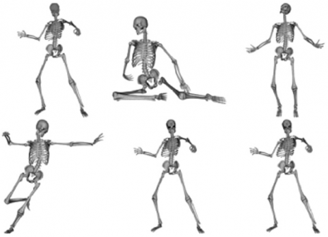
The body interaction reconstruction model [17] was established for wrong motion correction in motion recognition. The first step to model construction lies in feature extraction. When the body is in motion, each posture has its unique features. The same motion may be recognized differently with different recognition systems. Here, the visual feature acquisition method was employed to distinguish the wrong motions. The structure feature model of human motions is illustrated in Figure 1 below.
Figure 1. Structure feature model of human motions
Assuming that the human skeleton in Figure 1 has N joints, the world coordinate systems A and B were constructed based on the Denavit-Hartenberg (D-H) notation [18] for the spatial pose of the mathematical model of the kinematics chain. The D-H method can handle the key steps of the mapping from the Descartes space. The contour features of human motions can be extracted with the structural feature model. The extracted image matrix can be expressed as:
${{E}_{edge}}=[l'{{'}_{mn}}]M\times N$ (9)
To recognize the wrong motions, the characteristic variables of each posture can be calculated as:
$l_{mn}^{''}=\frac{|l_{mn}^{''}-\min \{l_{mn}^{''}\}|}{{{E}_{edge}}},(a,b)\in W$ (10)
where, W is a 3×3 window centered on the edge intensity (m, n). Through the analysis on the structural features of human motions, the background image B of an athlete (x, y)(x∈[0,W-1],y∈[0,H-1]) can be extracted from the background of the human motion image. Then, the background image B and the target image I were divided into (W/2)×(H/2) grids. Each grid can be described as:
$P(i,j)(i\in [0,\operatorname{int}({W}/{2}\;)-1],j\in [0,\operatorname{int}({H}/{2}\;)-1])$ (11)
where, W and H are the width and height of the human motion image, respectively. Each grid was imported to the structural feature model of human motions, and sorted according to the background image, thus completing the visual reconstruction process.
The visual features of the wrong motions were analyzed based on the visual reconstruction. Without changing the meaning of the parameters, the grid pheromone of the edge contour of a single frame in the human motion image can be obtained as:
$\min F(x)=\left(f_{1}(x), f_{2}(x), \ldots, f_{m}(x)\right)^{T}$
s.t. $g_{i} \leq 0, i=1,2 \ldots, q, h_{j}=0, j=1,2, \ldots, p$ (12)
where gi and hj are the moments of inertia of the body around the y-axis and the x-axis, respectively; q and p are the length and the width of the motion trajectory network, respectively; fm(x) is the pixel intensity of the edge corner point.
The grid pheromones were clustered to obtain the wrong feature information of the human motion image, and the feature information was filtered to perform curve segmentation on the wrong motion features. To analyze the wrong amplitude features, it is necessary to set up the following 3D viewpoint switching equations:
$\begin{align} & \overset{.}{\mathop{{\dot{x}}}}\,=V\cos \theta \cos \Psi ,\text{ }\overset{.}{\mathop{y}}\,=V\sin \theta \\ & \overset{\cdot }{\mathop{z}}\,=-V\cos \theta \sin {{\Psi }_{v}} \\ \end{align}$ (13)
$\overset{\cdot }{\mathop{\vartheta }}\,={{\omega }_{y}}\sin \gamma +{{\omega }_{2}}\cos \gamma $ (14)
where, x, y, z are the centroid coordinates of the human motion image; ψv is the switching angle of the motion region. Figure 2 shows the process of the visual analysis on wrong motions.
Figure 2. The process of the visual analysis on wrong motions
The visual reconstruction and feature analysis pave the way for 3D visual recognition of the wrong motions of athletes. To enhance the reconstruction effect, the distribution of each modeling point should be obtained by a suitable corner matching method and the motions should be discriminated. Hence, the author proposed a 3D visual recognition method based on the contourlet domain edge detection, which is implemented as follows.
For a grayscale image on human motions g(x, y), a small sub-region $w \in g$ was extracted from the image, and the sub-region image was moved both horizontally and vertically. The displacements are respectively denoted as x and y. The square of the grayscale change through the movement can be computed as:
$g(x, y)=\left\{\begin{array}{ll}b_{0}, & f(x, y)<T \\ b_{1}, & f(x, y) \geq T\end{array}\right.$ (15)
Here, corner feature acquisition of body boundary contour is carried out through scale-invariant feature transform (SIFT). The grayscale of all frames at (x, y) can be calculated as:
$P(i, j)=\left\{\begin{array}{ll}1, & \left|\frac{1}{4}\left[B_{G}-I_{G}\right]\right|-Y_{G} \times g(x, y)>0 \\ 0, & \text { otherwise }\end{array}\right.$ (16)
Next, the contourlet domain edge detection algorithm was designed. The image contourlet domain matrix was established in the form of a Hessian matrix:
$\mathrm{D}=\left[\begin{array}{cc}I_{x}^{2} & I_{x} I_{y} \\ I_{x} I_{y} & I_{y}^{2}\end{array}\right]$ (17)
where, $I_{x}$ is the wrong feature of the human motion image; $I_{y}$ is the vertical amplitude of a motion; $I_{x} I_{y}$ is the correlation between the wrong motion and the correct motion. Through the first-order Taylor expansion, the eigenvector of the contourlet domain can be obtained as:
$\varphi (t)=\lg {{p}_{t}}(1-{{p}_{t}})+\frac{{{H}_{t}}}{{{P}_{t}}}+\frac{{{H}_{L-1}}-{{H}_{t}}}{1-{{P}_{t}}}$ (18)
${{P}_{t}}=\sum\limits_{i=0}^{t}{{{P}_{i}}}$ (19)
The following equation can be obtained from Eqns. (18) and (19):
${{H}_{t}}=-\sum\limits_{i=0}^{t}{{{p}_{i}}\lg {{p}_{i}}}$ (20)
Thus, the grayscale change of the sub-region was converted into two eigenvalues of the structural matrix M(x, y): λ1 and λ2. Then, the local structure matrix M was taken as a correlation function, and used to judge whether the detection point (x, y) is a corner point of the image. The judgement was made based on the two eigenvalues in the local structure matrix M. Let pm(m) be the probability density function of the non-subsampled contourlet transform (NSCT) and pn(n) be the probability density function of noise. Then, the relationship of the SIFT corner point of the edge feature can be obtained as:
$\frac{{{p}_{m}}(m)}{{{p}_{n}}(n)}=\frac{\partial \cdot \beta }{{{(\partial +\beta )}^{2}}}=\frac{\gamma }{{{(\gamma +1)}^{2}}}$ (21)
where,
$\frac{\gamma }{{{(\gamma +1)}^{2}}}<\frac{{{\gamma }_{0}}}{{{({{\gamma }_{0}}+1)}^{2}}}$ (22)
where, I(x, y) is the grayscale of the edge feature at (x, y); L(x, y, σ) is the information entropy space; G(x, y, σ) is the modal tracking corner information of the edge feature.
Through the above steps, the contour curve of the wrong motions was drawn by the SIFT corner detection algorithm, and the contourlet domain was smoothed, which marks the end of the 3D visual recognition of wrong motions.
This section attempts to verify the effectiveness of the proposed method in wrong motion recognition and 3D feature analysis. Thus, a 3D kinematics model of human motions was constructed and the 3D characteristic variables were calculated. Table 1 lists the variables of the 3D kinematics model for athletes.
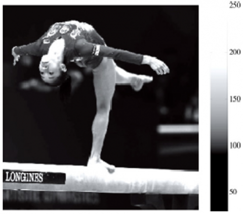
According to the 3D model parameters, the motion features were collected from the human motion image. During the feature acquisition, the jitter was -130Bm, the resolution was 0.5m and the pixel number was 540*400. The color tone of wrong recognition was divided into 16 levels. If a wrong recognition happens, the grayscale will be set to white and the interference signal will be added. For every 1s increase in the signal near 70s, the motion features were disturbed for 1s. Based on these settings, the author plotted a 3D visual image (Figure 3) from the original human motion image.
Table 1. The variables of the 3D kinematics model for athletes
|
i |
qi/r |
$\alpha_{i} / r$ |
$\alpha_{i}^{\prime} / m m$ |
$\boldsymbol{d}_{i} / \boldsymbol{m} \boldsymbol{m}$ |
BM |
|
1 |
q1 |
-π/2 |
Is |
1 |
[-π/4,π/2] |
|
2 |
q2-π/2 |
-π/2 |
1 |
0 |
[-π/4,π/2 |
|
3 |
q3+π/2 |
π/2 |
0 |
Iu |
[-π/2,π/2] |
|
4 |
q4 |
-π/2 |
0 |
0 |
[0,π/4] |
|
5 |
q5 |
π/2 |
0 |
If |
[0, π/2] |
|
6 |
q6+π/2 |
-π/2 |
0 |
0 |
[-π/2,π/4] |
|
7 |
q7 |
π/2 |
Ih |
0 |
[-π/2,π/4] |
Note: i is the number of variables; $q_{i}$ and $\alpha_{i}$ are the spatial coordinates of the athlete during the exercise; $\alpha_{i}^{\prime}$ and $d_{i}$ are spatial position and motion distance of the athlete during the exercise, respectively; BM is the body motion constraint.
Figure 3. Original human motion image
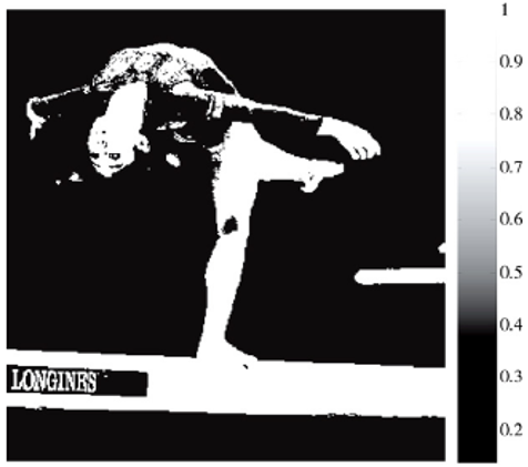
As shown in Figure 3, the original human motion image contained some wrong amplitude features. To correct the amplitude, it is necessary to identify and extract the wrong motions. The visual reconstruction and feature analysis of human motion were carried out. The edge detection features were extracted by edge detection algorithm. The extraction effect of wrong amplitude features is shown in Figure 4 below.
Figure 4 shows that our algorithm effectively extracted and recognized wrong amplitude features, and enhanced the ability of motion correction and recognition. Under the edge detection of the contourlet domain, the proposed algorithm was compared with the improved inverse kinematics algorithm in terms of the wrong motions. The original image, the result of the contrastive algorithm and that of our algorithm are respectively displayed in Figures 5~7 below.
Obviously, our algorithm outperformed the improved inverse kinematics algorithm in motion amplitude tracking. The good performance of our algorithm is mainly attributable to the advantage in calibration. The contrastive algorithm calibrates the camera imaging plane according to the pinhole camera model.
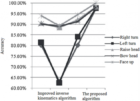
Figure 8 compares the 3D visual recognition results of the two algorithms on wrong motions in sports training. Our algorithm still outshined the contrastive algorithm in all aspects.
Figure 4. Extraction effect of wrong amplitude features
Figure 5. Original image
Figure 6. Result of the contrastive algorithm
Figure 7. Result of our algorithm
Figure 8. 3D visual recognition results of the two algorithms on wrong motions
This paper designs a 3D visual image recognition method based on contourlet domain edge detection, and applies it to the recognition of athlete’s wrong motions in sports training. Firstly, the visual reconstruction and feature analysis of human motions were carried out, and the edge detection features were extracted by edge detection algorithm. Then, a 3D visual motion amplitude tracking method was proposed based on improved inverse kinematics. The simulation results show that the proposed algorithm can effectively realize the recognition of 3D visual images of athlete motions, and improve the correction and judgment ability of athlete motions.
This paper was supported by the Science Research Plan Project of Shaanxi Province Education Department (Grant No.: 18JK0025) and the Key Subsidizing Item of Scientific Research of Baoji University of Arts and Science (Grant No.: ZK2017005).
[1] Tao, H., Lv, J., Xie, Q., Sun, H., Yuan, Q. (2017). A novel human behaviour information coding method based on eye-tracking technology. Traitement du Signal, 34(3-4): 153-173. https://doi.org/10.3166/TS.35.153-173
[2] Liu, K.C., Chan, C.T. (2017). Significant change spotting for periodic human motion segmentation of cleaning tasks using wearable sensors. Sensors, 17(1): 187. https://doi.org/10.3390/s17010187
[3] Ribnick, E., Sivalingam, R., Papanikolopoulos, N., Daniilidis, K. (2012). Reconstructing and analyzing periodic human motion from stationary monocular views. Computer Vision and Image Understanding, 116(7): 815-826. https://doi.org/10.1016/j.cviu.2012.03.004
[4] Lüthi, A., Böttinger, G., Theile, T., Rhyner, H., Ammann, W. (2006). Freestyle aerial skiing motion analysis and simulation. Journal of Biomechanics, 39(S1): S186. https://doi.org/10.1016/S0021-9290(06)83664-X
[5] Kesorn, K., Poslad, S. (2011). An enhanced bag-of-visual word vector space model to represent visual content in athletics images. IEEE Transactions on Multimedia, 14(1): 211-222. https://doi.org/10.1109/tmm.2011.2170665
[6] Kolekar, M.H. (2011). Bayesian belief network based broadcast sports video indexing. Multimedia Tools and Applications, 54(1): 27-54. https://doi.org/10.1007/s11042-010-0544-9
[7] Panigrahi, S.K., Gupta, S. (2018). Automatic ranking of image thresholding techniques using consensus of ground truth. Traitement du Signal, 35(2): 121-136. https://doi.org/10.3166/TS.35.121-136
[8] Yu, C.Y., Zhang, W.S., Yu, Y.Y., Li, Y. (2013). A novel active contour model for image segmentation using distance regularization term. Computers & Mathematics with Applications, 65(11): 1746-1759. https://doi.org/10.1016/j.camwa.2013.03.021
[9] Dirami, A., Hammouche, K., Diaf, M., Siarry, P. (2013). Fast multilevel thresholding for image segmentation through a multiphase level set method. Signal Processing, 93(1): 139-153. https://doi.org/10.1016/j.sigpro.2012.07.010
[10] Sun, G., Bin, S. (2018). A new opinion leaders detecting algorithm in multi-relationship online social networks. Multimedia Tools and Applications, 77(4): 4295-4307. https://doi.org/10.1007/s11042-017-4766-y
[11] Jiang, Y., Xu, Y., Liu, Y. (2013). Performance evaluation of feature detection and matching in stereo visual odometry. Neurocomputing, 120: 380-390. https://doi.org/10.1016/j.neucom.2012.06.055
[12] Zhang, Z., Wu, Q., Zhuo, Z., Wang, X., Huang, L. (2013). Fast wavelet transform based on spiking neural network for visual images. International Conference on Intelligent Computing, Nanning, China, pp. 7-12. https://doi.org/10.1007/978-3-642-39678-6_2
[13] Pae, S.I., Ponce, J. (2001). On computing structural changes in evolving surfaces and their appearance. International Journal of Computer Vision, 43(2): 113-131. https://doi.org/10.1023/a:1011170702891
[14] Barris, S., Button, C. (2008). A review of vision-based motion analysis in sport. Sports Medicine, 38(12): 1025-1043. https://doi.org/10.2165/00007256-200838120-00006
[15] Fang, Q., Meaney, P.M., Paulsen, K.D. (2006). Singular value analysis of the Jacobian matrix in microwave image reconstruction. IEEE Transactions on Antennas and Propagation, 54(8): 2371-2380. https://doi.org/10.1109/TAP.2006.879192
[16] Chen, H., Yu, S. (2017). A stereo camera tracking algorithm used in glass-free stereoscopic display system. Journal of Computer-Aided Design & Computer Graphics, 29(3): 436-443.
[17] Zhang, Y., Tao, R., Zhang, F. (2015). Key frame extraction based on spatiotemporal motion trajectory. Optical Engineering, 54(5): 050502. https://doi.org/10.1117/1.OE.54.5.050502
[18] Li, L., Huang, Y., Guo, X.X. (2019). Kinematics modelling and experimental analysis of a six-joint manipulator. Journal Européen des Systèmes Automatisés, 52(5), 527-533. https://doi.org/10.18280/jesa.520513