Mouad Garziad* | Abdelmjid Saka
OPEN ACCESS
The rider plays an important role in the stability and control of two-wheeled vehicles. The rider model must be designed carefully according to the physical and geometric features of the target two-wheeled vehicle. This paper aims to disclose how the rider affects the control and stability of two-wheeled vehicles. First, the two-wheeled vehicle-rider system was modelled and subjected to dynamic analysis. Next, the motion equations of a two-wheeled vehicle were linearized with forwarding velocity and small disturbances in displacement. Further, the genetic algorithm (GA) was introduced to optimize the parameters of the proportional-integral-derivative (PID) controller, taking the steering torque and lean torque from the rider as the inputs. Finally, the PID controller was compared with the PI and PD controllers through simulation of a two-wheeled vehicle-rider system. The results show that the rider plays the role of derivation action; the motion of the upper body of the rider has a secondary impact on vehicle stability; the rider can stabilize the vehicle through both lean and steering torques generated by his/her upper body movements.
two-wheeled vehicle, rider, lean torque, steering torque, proportional-integral-derivative (PID) controller
The stability of the two-wheeled vehicle is an important aspect in the domain of mechanical engineering and control theory. It is significant due to its direct impact on the safety and comfortability of the rider; therefore, is an area that has attracted the attention of researchers who aimed at securing as granting contentment of the rider. Those researchers have contributed in the enlargement of the theory of the two-wheeled vehicles, and in the description of the critical factors and parameters that influence on the safety, comfort, and efficiency of driving of the two-wheeled vehicles. They accomplished with mathematical and physical models more accurate and reliable to describe this type of vehicle. So far, the majority of literature focuses on mathematical models, both with simplified or linearized, and complex models. The aim behind these contributions is to describe specific aspects of the two-wheeled vehicles dynamic as to define the phenomena of instability mode [1, 2]. Whipple [3] published one of the first articles that discussed mathematical modeling in 1899. He established a nonlinear equation for a bicycle model to examine its stability. In this respect, several researchers have based their research on these dynamic equations. However, in literature, the rider and his influences on the dynamics of two-wheeled vehicles are treated unrealistically and modeled as simplified or passive models as a rigid body [4–11] attached to the body frame of two-wheeled vehicles while other physical models were modeled as a simplified biomechanical of a rider [12-14]. As an alternative, the third development was an artificial system acting as a steering system. None of these approaches of modeling was representative due to its low potential action of a rider while controlling the two-wheeled vehicles. The main reason for not using these kind of models exist in the difficulty of integration of the driver model with sufficient degrees of freedom. Among the various models developed in the literature, Keppler [15] was one from the researcher to identify the parameters of rider, the characteristics and the influence of the rider’s biomechanical parameters on the dynamic ride stability. Moreover, Zhu et al. [16] analyzed the rider’s effect on the motion of a motorcycle taking into consideration of the leaning motion of the rider’s upper body and rider’s arm, in steady-state turning. Furthermore, Chung et al. [17] discuss the riding comfort of the electric motorcycles-rider to follow a desired path to maintain the stabilization of the model. The research considered the biomechanical proprieties and the rider model, which is composed of 12 rigid bodies.
Our study aims to explain, in the first section, the effect of the rider in the stability of bicycle and the choice of the type of controller. The research goes further in demonstrating that the rider is able to play the role of integral or derivative action. The article adopts evaluating and comparative approaches that examine the performance of PI, PD, and PID. The second section gives a brief introduction about the kinematic and dynamic of the proposed model. Then, the third section describes the proposed strategy of control of a bicycle - rider system, based on PID, to generate the required roll and steer angle. The fourth section shows the simulation results. The last section provides a conclusion that discusses the results and findings of this study.
2.1 System description
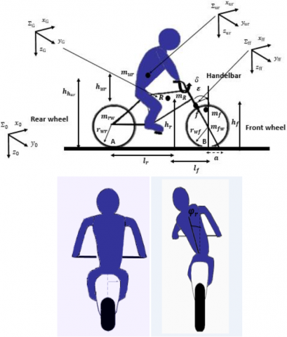
In this study, the dynamic of the two-wheeled vehicle-rider system is extended from the nine degrees of freedom two-wheeled vehicle model presented in previous work [18-20]. The Figure 1 shows the model of the two-wheeled vehicle-rider system. The model used in this research consists of front forks that contains handlebars and front wheel; rear frame contains rear wheel, the rider body, and two-wheeled vehicle body, the rider’s upper body can lean relative to the two-wheeled vehicle frame. The center of gravity of the rigid body is represented by: $m_{\mathrm{R}}, m_{\mathrm{f}}, m_{\mathrm{fw}}, m_{\mathrm{rw}},$ and $m_{\mathrm{ur}}$.
Figure 1. Two wheeled vehicle – rider model
The two-wheeled vehicle is described by both its wheel radii $r_{r w}$ and $r_{f w}$. The position of the two-wheeled vehicle is determined by coordinates x and y of the contact point of the rear wheel taking into consideration the $x y$ plane coincides with the ground, the height to the ground plane are $h_{f}$ and $h_{r}$. The motion of the two-wheeled vehicle is referred to the inertial reference frame $\Sigma_{0}\left(\mathrm{O} ; \mathrm{X}_{0} ; \mathrm{Y}_{0} ; \mathrm{Z}_{0}\right)$ fixed on the ground, a reference frame $\Sigma_{\mathrm{R}}\left(\mathrm{O} ; \mathrm{X}_{\mathrm{R}} ; \mathrm{Y}_{\mathrm{R}} ; \mathrm{Z}_{\mathrm{R}}\right)$ mounted on the model at point $G,$ and a frame $\Sigma_{\mathrm{ff}}\left(\mathrm{O} ; \mathrm{X}_{\mathrm{f}} ; \mathrm{Y}_{f} ; \mathrm{Z}_{\mathrm{f}}\right)$ placed on the front fork. The coordinate $\Sigma_{\mathrm{e}}$ is obtained by rotating about a rake angle $\varepsilon$ and $\delta$ steering angle, the frame $\Sigma_{\mathrm{ur}}\left(\mathrm{O} ; \mathrm{X}_{\mathrm{ur}} ; \mathrm{Y}_{\mathrm{ur}} ; \mathrm{Z}_{\mathrm{ur}}\right)$ is used to describe the motion of the rider upper body as shown in Figure 1. The kinematics of rider is described in terms of the motion of the upper body, where the rider model consists of two rigid bodies; the upper body, and the lower body of the rider respectively. The main motion of the rider model is leaning of the body this motion is modeled by torques.
2.2 Dynamic analysis of the two wheeled vehicles
To generate the dynamic equations that describe the motion of the two Wheeled Vehicle-Rider, we used the Lagrange approach: the main step is to develop the kinetic and potential energy of the rigid bodies after expanding the Lagrangian to the second-order, the kinematic and dynamic modeling of the two Wheeled Vehicle–Rider system is discussed by Chu and Chen [21].
The kinetic energy is represented in the following equation:
$T=\frac{1}{2} m_{f w} \dot{r}_{f w} \dot{r}_{f w}+\frac{1}{2} m_{r w} \dot{r}_{r w} \dot{r}_{r w}+\frac{1}{2} m_{R} \dot{r}_{R} \dot{r}_{R}+$
$\frac{1}{2} m_{u r} \dot{r}_{u r} \dot{r}_{u r}+\frac{1}{2} m_{F} \dot{r}_{F} \dot{r}_{F}+\frac{1}{2} \Omega_{f w}^{T} I_{f w} \Omega_{f w}+\frac{1}{2} \Omega_{r w}^{T} I_{r w} \Omega_{r w}+$
$\frac{1}{2} \Omega_{R}^{T} I_{R} \Omega_{R}+\frac{1}{2} \Omega_{F}^{T} I_{F} \Omega_{F}+\frac{1}{2} \Omega_{u r}^{T} I_{u r} \Omega_{u r}$ (1)
The potential energy is:
$V=m g h$ (2)
where,
$V=-g^{T}\left(m_{f w} r_{f w}+m_{r w} r_{r w}+m_{F} r_{F}+m_{R} r_{R}+m_{u r} r_{u r}\right)$ (3)
The Lagrange Equations are then:
$\frac{d}{d t}\left(\frac{\partial L}{\partial \dot{q}_{i}}\right)-\frac{\partial L}{\partial q_{i}}=Q_{i}$ (4)
where, $L=T-V,$ and $Q_{i}$ are the non-conservative forces.
We can linearize the equations of motion for a two-wheeled vehicle with forwarding velocity v and small disturbances about its displacements.
The Proposed lateral dynamics model of the two-wheeled vehicle-rider is defined by the linearized equations of motion:
$M \ddot{q}+\left(C_{0}+v C_{1}\right) \dot{q}_{1}+\left(K_{0}+v^{2} K_{2}\right) q=f$ (5)
where,
The state vector of system is : $x=\left[\varphi, \dot{\varphi}, \delta, \dot{\delta}, \varphi_{r} \dot{\varphi}_{r}\right]^{T}$, and the control input vector is : $u=\left[0, T_{\delta}, T_{\varphi_{r}}\right]$.
It is important to write the equations in matrix form for the case of two-second order differential equation:
$[M]\left[\begin{array}{c}{\ddot{\varphi}} \\ {\ddot{\delta}} \\ {\ddot{\varphi}_{r}}\end{array}\right]+v\left[C_{1}\right]\left[\begin{array}{c}{\dot{\varphi}} \\ {\dot{\delta}} \\ {\dot{\varphi}_{r}}\end{array}\right]+\left\{g\left[K_{0}\right]+v^{2}\left[K_{2}\right]\right\}\left[\begin{array}{c}{\varphi} \\ {\delta} \\ {\varphi_{r}}\end{array}\right]+[C]\left[\begin{array}{c}{\dot{\varphi}} \\ {\dot{\delta}} \\ {\dot{\varphi}_{r}}\end{array}\right]+[K]\left[\begin{array}{c}{\varphi} \\ {\delta} \\ {\varphi_{r}}\end{array}\right]=\left[\begin{array}{c}{0} \\ {T_{\delta}} \\ {T_{\varphi_{r}}}\end{array}\right]$ (6)
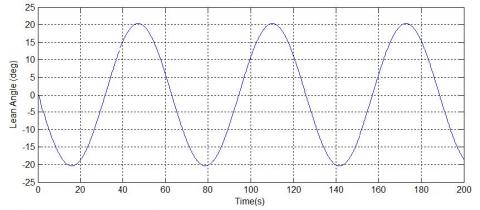
Figure 2. Lean angle of two wheeled vehicle – 5m/s
Figure 3. Lean angle of rider– 5m/s
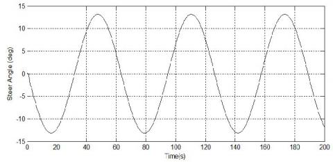
Figure 4. Steer angle – 5m/s
The values of the parameters of the system are mentioned in the appendix 1 (Table 1).
The matrix $\boldsymbol{M}, \boldsymbol{C}_{\mathbf{0}}, \boldsymbol{C}_{\mathbf{1}} \boldsymbol{K}_{\mathbf{0}}, \boldsymbol{K}_{\mathbf{2}}$ are defined in Appendix 2.
The results of simulations in Figure 2, 3 and 4 show the lean angle and steer angle of the two-wheeled vehicle, and lean angle of rider, without any control action of rider.
3.3 Stability analysis
The behavior of the system is examined by plotting the eigenvalues for the linearized system and explaining the relevant two-wheeled vehicle modes of instability as shown in Figure 5. To illustrate this concept, we analyzed the eigenvalue to determine the different mode of instability as the self-stabilizing area of an uncontrolled two-wheeled vehicle.
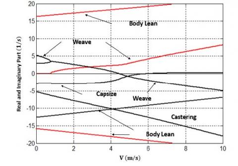
Figure 5. Eigenvalues and stability of system, with positive real parts of eigenvalues, negative real parts of eigenvalues, and imaginary parts of eigenvalues
The Eigenvalues from the linearized stability analysis where red line represents the imaginary part of the eigenvalues and black lines presents the real part of the eigenvalues, in the forward speed range 0-10 m/s. The speed range for the stability of the two-wheeled vehicle is from $v_{w}<\mathrm{v}<v_{c}$.
There are two main velocities indicated in Figure 5. One is the weave velocity $v_{w}$ at which the weave mode becomes stable, and the other is the capsize velocity at which the capsize mode becomes unstable $v_{c}$, the weave mode begins at zero velocity, the self-stability range disappears.
The weave mode shows only a small torsion component of the upper body that adds to the roll and steering components that are similar to the ones of the benchmark model [2]. The castering mode shows a small torsion component that adds to the steer component. The new torsion mode shows a small steer component.
To develop control design for lateral configuration, the section aimed at comparing the three control structures for lateral guidance based solely on PID. The goal is to find a method of regulating the lateral dynamics of the vehicle valid throughout the speed range of $0-10 m / s$.
The state-space representation is then given by:
$\dot{x}=A x+B u$
$y=C x+D$ (7)
The vector $x=\left[\varphi, \dot{\varphi}, \delta, \dot{\delta}, \varphi_{r} \dot{\varphi}_{r}\right]^{T}$ represents the state vector of the dimension $(n x 1)$, $u$ the input vector of the dimension $(r x 1)$, $y$ the output vector of the dimension $(\mathrm{m} \mathrm{x} 1)$, $A$ the system matrix of the dimension $(n x n)$, $B$ the input matrix of the dimension $(n x m)$, $C$ the output matrix of the dimension $(p x n)$ and $D$ the matrix of passage of the dimension $(p x m)$.
The control input vector is $u=\left[0, T_{\delta}, T_{\varphi_{r}}\right]$.
The rider lean and steer torque were the inputs for the controller represented into multiple sinusoidal signals. The stabilizing controller outputs were the roll and steer rate angle.
Genetic Algorithm (GA) based on the PID controller was proposed for tuning optimized PID parameters, under multiple sinusoidal inputs.
The PID is modeled by two input, which are:
$T_{\delta}=-K_{\delta_{P}}\left(\delta_{r e f}-\delta\right)-K_{\delta_{I}} \int\left(\delta_{r e f}-\delta\right)+K_{\delta_{D}} \dot{\delta}$ (8)
$T_{\varphi_{r}}=-K_{\varphi_{P}}\left(\varphi_{r e f}-\varphi\right)-K_{\varphi_{I}} \int\left(\varphi_{r e f}-\varphi\right)+K_{\varphi_{D}} \dot{\varphi}$ (9)
where, $T_{\delta}$ the steering torque control used to obtain a desired steering angle, $\delta$ is the steer angle and $\delta_{r e f}$ is the desired steer angle, where $K_{\delta_{P}}, K_{\delta_{I}},$ and $K_{\delta_{D}}$ are respectively the proportional, the derivative and the integral gain. $T_{\varphi_{r}}$ represent the steering lean torque used to obtain a desired roll angle, $\varphi$ is the lean angle and $\varphi_{r e f}$ is the desired lean angle, where $K_{\varphi_{P}}$ $K_{\varphi_{I}},$ and $K_{\varphi_{D}}$ are respectively the proportional, the derivative and the integral gain.
The Figure 6 illustrate the structure of PID controller.
Figure 6. Block diagram design of Controller
The figures below show simulations which perform both roll rate and steers rate angles. The controller parameters were obtained based on a Genetic Algorithm.
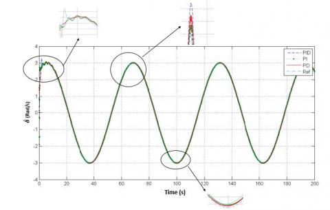
Figure 7. Steer rate angle (rad/s)
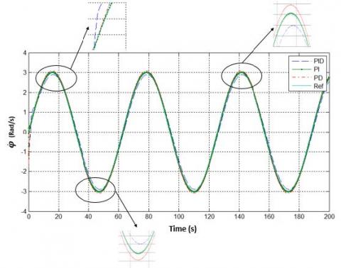
Figure 8. Roll rate angle (rad/s)
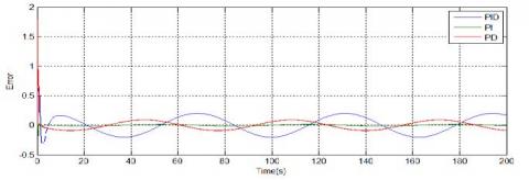
Figure 9. Lean angle error
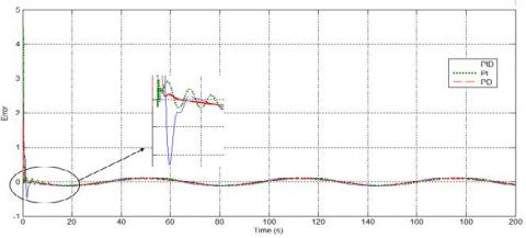
Figure 10. Steer angle error
Figure 7 and 8 illustrate the control results both in steer angle and roll angle.
The simulation results prove that the controller ensures a good follow-up of the maneuvers in roll and in steering action of rider upper body.
The performance of PI, PD and PID controller is analyzed and compared throughout the simulations that are mentioned before. To determine which control strategy that delivers better performance and to determine the action of the rider, we established a comparative assessment between these controllers, Figure 9 and 10 represent a clear vision of the result of error between the three controllers.
These simulations results illustrate a good response obtained by tuning the PI controller. The results proved that the rider is able to play the role of derivative action.
The results show that the motion of the upper part of the rider body has a secondary impact on the stability. In other words, and based on Figure 5, the integration of lean angle of the upper part of the rider makes it possible to stabilize the Capsize mode, which is characterized by the appearance of a new additional eigenvalue and described by a negative real part that is attributed to the lean motion of rider. As a result, the weave mode shows only a small twisting component of the upper body that adds to the roll and steering components, which are closely similar to the Whipple Bicycle model.
Since the stability of the two-wheeled vehicle is a significant field of mechanical engineering and control theory, we have chosen to break down some aspects in four sections. The first section discussed the kinematic and dynamic equation of two-wheeled vehicle- rider utilizing Lagrange approach equations with holonomic constraints. The second part that followed dealt with the analyses of the eigenvalues and stability of the two-wheeled vehicle–Rider model. The third part targeted the implementation of PID Controller and the determination of which control strategy delivers better performance between three controllers: PID, PD and PI, for controlling using for control two input, the steering and upper body lean torque. The main goal behind this comparison was to identify if the rider can affect the choice of the controller and illustrate if the rider has the ability to play the role of the integral or derivative action. The fourth section discussed the results and analysis, which proved that the rider contributes in the derivative action. In this respect, it is recommended for future studies to focus on evaluating general rider’s characteristics and abilities such as acquisition of information, visual, auditory, perception, reaction time and neuromuscular dynamics, also, it’s interesting to implement some algorithm and tools to improve the safety and to prevent accidents to recognize relevant driving characteristics-parameters, such as driving style, characteristics of the road, the treatment of curves, etc.
|
$a$ |
Trail |
|
$R_{w f}$ |
Radius of the front wheel |
|
$R_{w r}$ |
Radius of the rear wheel |
|
$W$ |
Wheelbase |
|
$l_{r}$ |
Horizontal distance from A |
|
$l_{f}$ |
Horizontal distance from B |
|
$h_{r}$ |
Vertical distance from A |
|
$m_{r}$ |
Mass rear frame |
|
$m_{f}$ |
Mass front frame |
|
$m_{rw}$ |
Mass rear wheel |
|
$m_{fw}$ |
Mass front wheel |
|
$\boldsymbol{\varepsilon}$ |
Caster angle |
|
$\varphi, \delta$ |
Roll , Steer angle |
|
$\varphi_{r}$ |
Roll angle of rider |
|
$h_{u r}, h_{h u r}$ |
Centre of mass of height body, height of the centre mass of trunk |
|
$g$ |
acceleration of gravity |
|
$S_{A}$ |
static moment |
|
$\left(x_{u r}, y_{u r}, Z_{u r}\right)$ |
Coordinate of rider upper body |
|
$k_{\varphi_{r}} C_{\varphi_{r}}$ |
Lean stiffness and damping |
|
$k_{\delta}, C_{\delta}$ |
Steer stiffness and damping |
[1] Meijaard, J.P. (2004). Derivation of the linearized equations for an uncontrolled bicycle. Internal Report, University of Nottingham, UK.
[2] Meijaard, J.P., Schwab, A.L. (2006). Linearized equations for an extended bicycle model. In III European Conference on Computational Mechanics, Springer, Dordrecht, pp. 772-772.
[3] Whipple, F.J. (1899). The stability of the motion of a bicycle. Quarterly Journal of Pure and Applied Mathematics, 30(120): 312-348.
[4] Chen, C.K., Chu, T.D., Zhang, X.D. (2019). Modeling and control of an active stabilizing assistant system for a bicycle. Sensors, 19(2): 248. https://doi.org/10.3390/s19020248
[5] Popov, A.A., Rowell, S., Meijaard, J.P. (2010). A review on motorcycle and rider modelling for steering control. Vehicle System Dynamics, 48(6): 775-792. https://doi.org/10.1080/00423110903033393
[6] Dialynas, G., Happee, R., Schwab, A.L. (2019). Design and hardware selection for a bicycle simulator. Mechanical Sciences, 10(1): 1-10. https://doi.org/10.5194/ms-10-1-2019
[7] Sharp, R.S. (2007). Motorcycle steering control by road preview. Journal of Dynamic Systems, Measurement, and Control, 129(4): 373-381. https://doi.org/10.1115/1.2745842
[8] Meyer, D., Zhang, W., Tomizuka, M. (2015). Sliding mode control for heart rate regulation of electric bicycle riders. In ASME 2015 Dynamic Systems and Control Conference. American Society of Mechanical Engineers Digital Collection.
[9] Moore, J.K., Hubbard, M., Schwab, A.L., Kooijman, J.D.G., Peterson, D.L. (2010). Statistics of bicycle rider motion. Procedia Engineering, 2(2): 2937-2942.
[10] Connors, B. (2009). Modeling and stability analysis of a recumbent bicycle with oscillating leg masses. University of California, Davis.
[11] Meijaard, J.P., Schwab, A.L. (2006). Linearized equations for an extended bicycle model. In III European Conference on Computational Mechanics, Springer, Dordrecht, pp. 772-772.
[12] Doria, A., Tognazzo, M. (2014). The influence of the dynamic response of the rider’s body on the open-loop stability of a bicycle. Proceedings of the Institution of Mechanical Engineers, Part C: Journal of Mechanical Engineering Science, 228(17): 3116-3132. https://doi.org/10.1177%2F0954406214527073
[13] Bulsink, V.E., Doria, A., Van, B.D., Koopman, B. (2015). The effect of tyre and rider properties on the stability of a bicycle. Advances in Mechanical Engineering, 7(12). http://dx.doi.org/10.1177/1687814015622596
[14] Doria, A., Marconi, E. (2018). A Testing Method for the prediction of comfort of city bicycles. In ASME 2018 International Design Engineering Technical Conferences and Computers and Information in Engineering Conference. American Society of Mechanical Engineers Digital Collection.
[15] Keppler, V., Solutions, B. (2010). Analysis of the biomechanical interaction between rider and motorcycle by means of an active rider model. In Proceedings, Bicycle and Motorcycle Dynamics 2010 Symposium on the Dynamics and Control of Single Track Vehicles, Delft, The Netherlands, pp. 20-22.
[16] Zhu, S.P., Murakami, S., Nishimura, H. (2012). Motion analysis of a motorcycle taking into account the rider's effects. Vehicle sys$tem dyna$mics, 50(8): 1225-1245. http://dx.doi.org/10.1080/00423114.2012.660166
[17] Lai, H.C., Liu, J.S., Lee, D.T., Wang, L.S. (2003). Design parameters study on the stability and perception of riding comfort of the electrical motorcycles under rider leaning. Mechatronics, 13(1): 49-76. https://doi.org/10.1016/S0957-4158(01)00082-4
[18] Chen, C.K., Dao, T.S. (2005). Dynamics and path-tracking control of an unmanned bicycle. In ASME 2005 International Design Engineering Technical Conferences and Computers and Information in Engineering Conference, American Society of Mechanical Engineers, pp. 2245-2254.
[19] Chen, C.K., Dao, T.S. (2006). Fuzzy control for equilibrium and roll-angle tracking of an unmanned bicycle. Multibody System Dynamics, 15(4): 321-346. https://doi.org/10.1007/s11044-006-9013-7
[20] Garziad, M., Saka, A. (2019). A comparative assessment between LQR and PID strategies in control of two wheeled vehicle. In International Journal of Engineering Research in Africa, 43: 59-70. https://doi.org/10.4028/www.scientific.net/JERA.43.59
[21] Chu, T.D., Chen, C.K. (2018). Modelling and model predictive control for a bicycle-rider system. Vehicle System Dynamics, 56(1): 128-149. https://doi.org/10.1080/00423114.2017.1346263