Youpeng Lu | Xiao Pei* | Changze Zhang | Haiyan Luo | Bin Liu | Zhide Ma
OPEN ACCESS
This paper aims to optimize the largescale complex multimodal transport path in an efficient and accurate manner. To this end, the genetic algorithm (GA) was embedded into the ant colony optimization (ACO), creating a dual pheromone hybrid algorithm. The GA guides and speeds up the ACO to avoid the local optimum trap and enhance the optimization ability. Considering the scale effect of transport cost, a combinatorial optimization model was established to minimize the cost under the constraints of delivery time and path capacity, and tested in largescale multimodal transport networks. The test results show that the hybrid algorithm converged to the optimal solution through 46.17% and 45.25% fewer iterations, and lowered the transport cost by 4.23% and 2.39% than the GA and ACO, respectively. In addition, the hybrid algorithm was relied on to explore the factors affecting path selection. The research findings lay a solid basis for decision-making on multimodal transport.
multimodal transport, path optimization, scale effect, genetic algorithm (GA), ant colony optimization (ACO)
Container Multimodal Transport (CMT) is so efficient that its standard logistics system can organically integrate multiple transport modes to achieve seamless joint of all logistics chains. Today, with the further development of “The Belt and Road” strategy, the CMT will usher in a new development opportunity.
By far, the studies both at home and aboard mainly focus on how to improve the combination of optimal path and transport mode in a constraint environment. Reddy and Kasilingman [1] took the lead in designing a linear model that aims to minimize the total transportation cost. It is believed that the total transportation cost includes inter-node and node transit expenses. Further, Moccia et al. [2] allowed for the influence from arrival, departure time points set for transportation services at the nodes and the full transport time limit when selecting the path. GrBener et al. [3] analyzed the two methods for building the multimodal transport network and designed the improved Martins algorithm for solution. Zhang et al. [4] developed the bi-objective optimization model most reliable at the minimization of total cost, and that integrate the Genetic Algorithm (GA) and the Simulated Annealing Algorithm (SA) for solution. Rekik and Mellouli [5] established the multi-objective model that took the service quality first. Wang and Wang [6] considered uncertain factors in the transportation process and implemented the optimization model under the fuzzy demand. Jiang and Zhang [7] improved the ACO for a successive solution by randomly selecting nodes and introducing pheromone update strategies using the generalized cost as the objective function. Literature usually involves transportation cost as continuous function, but ignores such a fact that average transportation cost tends to decrease progressively with the increase of shipment volume in the practical transport process. As for the transportation time, it is almost impossible to differently consider the arrival and node time limits, only whichever of both.
Based on the results of previous studies, this paper involves the transportation economy “scale effect”, time window and path capacity constraints. The continuous piecewise linear function is used to express the transportation cost to make the model more adaptable to practical transportation process. The concept of "dual pheromone" is proposed to optimize the path and transportation mode. This is the GA-ACO hybrid algorithm that integrates the ACO and the GA which, as proved in practice, is feasible and effective.
In this paper, the main structure includes the following four sections: Section 1 describes the Problem description and modeling; Section 2 elaborates the hybrid algorithm to fill the gaps of other algorithms, for example, it is prone to local optimum; Section 3 affirms by an example that the hybrid algorithm is feasible and effective, and discusses the influence of traffic volume, transportation time limit and path capacity on path selection; Section 4 gives the Conclusion of the full text.
2.1 Model assumptions
(1) In the inland cities, for example, only two modes of transportation, roads and railways, are considered, and only one of both can be used between any two nodes;
(2) The transfer of transportation modes can only occur at the node. Except for the nodes O and D, any node can allow the transfer of transportation modes, but only once at most.
(3) The carrier only undertakes one logistics task at a time, which can not be split halfway.
(4) The traveling time involves the route length. The railway transportation will be limited by the timetable, that is, there is a specified time for arrival or departure, but no such constraint on road transportation;
(5) Transit cost and time limit have a linear relation with the traffic volume, and the facilities at any node should meet the requirements of the transit process.
2.2 Model description
Assume there is an undirected graph G= (V, E, K), where V is the set of nodes in the transport network; E is the set of transport segments; K is the set of transport modes. There are the goods of the transport volume q that require to be transported from the starting point O to the destination D.
First, the transport cost should be considered. Generally, the greater the shipment volume, the lower the transport cost allocated to each unit of goods. On every road segment (i, j), the relationship between transport cost and shipment volume can be expressed by continuous piecewise linear function. The shipment volume is divided into R linear segments. For r ∈R={1,2,…,|R|}, the intercept $f_{i j}^{k r} \in F_{i j}^{k}$ represents the fixed cost; the slope $c_{i j}^{k r} \in C_{i j}^{k}$ represents the variable cost; $m_{i j}^{k r}$ and $m_{i j}^{k(r-1)}$ are upper and lower limits of each segment; and $\left.c_{i j}^{k 1}>c_{i j}^{k 2}>\cdots>c_{i j}^{k r}, f_{i j}^{k r}=f_{i j}^{k r-1}+c_{i j}^{k (r-1)}-c_{i j}^{k r}\right) m_{i j}^{k(r-1)}$.
For transport time, assume $A_{i}^{k}, D_{i}^{k}, S_{i}^{k}$ are actual arrival, planed departure and actual transit time points for transport mode k at node i, respectively, it is easy to know the actual departure time of each node can be represented by $\max \left\{D_{i}^{k}, A_{i}^{k}+S_{i}^{k}\right\}$.
Other parameters are defined as follows:
$x_{i j}^{k}=\left\{\begin{array}{l}{1 \text { Goods are transported from nodes } i \text { to } j \text { using the transport mode } k} \\ {0 \text { Other transport mode is used }}\end{array}\right.$
$y_{i}^{k l}=\left\{\begin{array}{l}{1 \text { Goods are transited from node }} \\ {0 \text { There is no transit }}\end{array}\right.$
$c_{i}^{k l}$—Goods are transited from transport modes k to l at node i
$q_{i j}^{k r}$—Traffic volume of goods between nodes (i.j)
$t_{i j}^{k}$—Transport time limit of goods from nodes i to j using the transport mode k
$T^{k}$—Overall time limit for transporting the goods
$\left[T_{e}^{k}, T_{l}^{k}\right]$—Arrival time limit in the transport process of goods.
As described above, the following mathematical model can be created:
s.t.
$\begin{align} & {{Z}_{1}} \\ & =\min \sum\limits_{i,j\in E}{\sum\limits_{k\in K}{\sum\limits_{r\in R}{\left( f_{ij}^{kr}+c_{ij}^{kr}q_{ij}^{kr} \right)x_{ij}^{k}+\sum\limits_{i,j\in E}{\sum\limits_{k,l\in K}{c_{i}^{kl}}}}}}y_{i}^{kl}q \\ \end{align}$ (1)
$\sum_{i} q_{i j}^{k r}-\sum_{j} q_{j i}^{k r}=\left\{\begin{array}{ll}{q} & {\text { if } i=O(k)} \\ {-q} & {\text { if } i=D(k)} \\ {0} & {\text { otherwise }} \\ {\forall(i, j) \in E,} & {i, j \in V, k \in K}\end{array}\right\}$ (2)
$m_{i j}^{k(r-1)} x_{i j}^{k} \leq q_{i j}^{k r} \leq m_{i j}^{k r} x_{i j}^{k} \quad \forall(i, j) \in E, k \in K, \quad r \in R$ (3)
$T_{e}^{k} \leq T^{k}=\sum_{i, j \in E} \sum_{k \in K}\left(\begin{array}{c}{\max \left\{D_{j}^{k}, A_{j}^{k}+S_{j}^{k}\right\}-} \\ {\max \left\{D_{i}^{k}, A_{i}^{k}+S_{i}^{k}\right\}}\end{array}\right) \leq T_{l}^{k}$ (4)
$\left(\max \left\{D_{i}^{k}, A_{i}^{k}+S_{i}^{k}\right\}+t_{i j}^{k}-A_{j}^{k}\right) q_{i j}^{k r}=0 \quad \forall(i, j) \in E, i \in V, k \in K$ (5)
$\sum_{k \in K} x_{i j}^{k} \leq 1 \quad \forall(i, j) \in E$ (6)
$\sum_{k \in K} \sum_{l \in K} y_{i}^{k l} \leq 1 \quad \forall i \in V$ (7)
$x_{i j}^{k}+x_{j v}^{l} \geq 2 y_{j}^{k l} \quad \forall i, j, v \in V ; \forall k, l \in K$ (8)
$x_{i j}^{k}, y_{i}^{k l} \in\{0,1\}$ (9)
where, Formula (1) is the objective function, representing that the total cost is the minimum; (2) and (3) are the traffic constraints, namely, (2) is the traffic balance condition, and (3) gives the upper and lower bounds of cost incurred on the selected path. It is known that $m_{i j}^{k|R|}$ is the upper limits of the volume between segments (i,j). The "Squeeze" can ensure that the traffic volume is zero if there is no cost incurred on a segment. (4) is the overall time window constraint. The early arrival of the goods will give rise to the inventory cost. Once delayed, penalty cost will be incurred; (5) is the relationship between the goods flow and the time variable. If there is traffic volume between the segments (i, j), individual time nodes have a closed relationship. (6) and (7) makes sure there is only one transport mode selected on a road segment, and only one active transit performed at a node. (8) makes it certain that the transportation is continuous, that is, if the transport mode is transferred from k to l at the node i, the transport mode adopted from node i-1 to node i is k, and l from node i to node i+1. (9) is an integer constraint, ensuring that the goods are not split.
2.3 Model transformation
The above is a single-objective optimization model with nonlinear constraints. To further streamline it, the constraint (4) can be transformed into a penalty factor added to the objective function, thereby reducing one constraint, as shown in Formula (10):
$f\left(T^{k}, q\right)=\left\{\begin{array}{ll}{a\left(T_{e}^{k}-T^{k}\right) q+b} & {T^{k}<T_{e}^{k}} \\ {0} & {T_{e}^{k}<T^{k}<T_{l}^{k}} \\ {e^{2\left(T^{k}-T_{l}^{k}\right) q/\left(T_{l}^{k}-T_{e}^{k}\right)}} & {T^{k}>T_{l}^{k}}\end{array}\right\}$ (10)
This is the time deviation penalty function relevant to deviation time and freight volume, $f\left(T^{k}, q\right)=a\left(T_{e}^{k}-T^{k}\right) q+b$ represents the warehouse cost of goods early arrived, and is a linear function; $f\left(T^{k}, q\right)=\delta^{2\left(T^{k}-T_{1}^{k}\right) q /\left(T_{l}^{k}-T_{e}^{k}\right)}$represents the penalty cost of goods arrived in unduly time, and is an exponential function, wherein a and b all are non-negative constants, $a \neq 0, \delta$is a constant greater than 1 (where a, b, δ take 2, 50, 1.1, respectively). Then the original objective function turns into
$\min \sum_{i, j \in E} \sum_{k \in K} \sum_{r \in R}\left(f_{i j}^{k r}+c_{i j}^{k r} q_{i j}^{k r}\right) x_{i j}^{k}+\sum_{i, j \in E, k, l \in K} c_{i}^{k l} y_{i}^{k l}+f\left(T^{k}, q\right)$ (11)
The constraints are (2), (3), and (5)-(9). Since the (5) is still a nonlinear constraint, the solution process gets very complicated when using the common commercial software. It is therefore necessary to design an intelligent algorithm for solving the objective [8].
3.1 Description
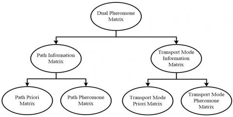
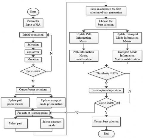
For this purpose, the GA-ACO hybrid algorithm is designed to solve the above problem. The dual pheromone matrix used for searching stores the paths and transportation modes separately. Refer to Figure 1 for specific structure. Given that the ACO algorithm converges at a slow rate due to less pheromone accumulation in the initial phase, the hybrid algorithm first uses the GA to generate better individual, records the combination of its path and transport mode, and used it as update basis for initial parameters of prior matrices of initial path and transport mode. Then, the ant colony generate the path and transport mode selection probabilities based on the prior and pheromone matrices, and select the next node and the transport mode using the roulette until the destination. The path and transportation mode pheromone matrices are updated with the results of every generation of elite ants, and the adaptive catastrophe operator is referenced based on the max and min ants to dynamically adjust the pheromone matrix and allow it timely jump out of the local optimum solution generated by the GA, narrow the gap between the best and the worst individual pheromones, enhance the random option of the ant colony for paths and transport modes, and improve the global search ability. The process of the hybrid algorithm is shown in Figure 2.
Figure 1. Information storage structure for dual pheromone hybrid algorithm
Figure 2. Process of dual pheromone hybrid algorithm
3.2 Genetic manipulation description
3.2.1 Genetic operator description
Coding: the chromosome is divided into two areas using the real-number parallel coding. Assume there are n urban nodes in the whole transportation network. The first area is the priority of each node, and n in length. The second area is arrangement of random transit modes with length n-1, so that this area does not need to be decoded. The whole area constitutes a chromosome of length 2n-1.
Decoding: For the decoding of the first area, the priority-based chromosome is used to decode [9]. Each node randomly generates different priorities. Then the priority of nodes is reachable in line with the connectivity comparison. Those nodes with higher priority are chosen. When the chromosome is traversing, an appropriate path is output and guaranteed for its connectivity. This method also thoroughly avoids the infeasible solution caused by the intersection and mutation. It has been proven to greatly improve the algorithm efficiency [10].
Fitness function: The algorithm fitness is the reciprocal of the objective function. The lower the objective function, the better the transport program.
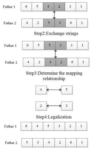
Crossover: The priority-based crossover is in fact to intersect the priorities. For the selected individuals, a partially consistent crossover method is performed [11], the crossover process is shown in Figure 3:
Figure 3. Crossover operation
Mutation: doppel mutation is performed on two areas of the chromosome.
Choice: The roulette selection method is used, and the probability that a chromosome is selected involves the fitness quality.
3.2.2 Genetic operator improvement strategy
Since the population more and more converges to better individuals after a certain number of iterations, the crossover has an obvious role at this time. The mutation operation continues to lead the population to converge to a better solution, so that it is feasible to use the crossover and mutation rates subjected to change with the number of iterations of the algorithm [12], as shown in Formulas (12) and (13):
Crossover rate: $p c_{i}=\max \left\{0.6, p c_{i-1}-0.05\right\}$ (12)
Mutation rate $p m_{i}=m i n\left\{0.7, p m_{i-1}+0.05\right\}$ (13)
where, pc0=0.8, pm0=0.2
3.3 Ant colony operation description
3.3.1 Dynamic pheromone update strategy:
To avoid the hybrid algorithm trapping in the local optimum solution at the very start, before the ant colony uses the dual pheromone matrix, set the initial pheromone quantity $τ_g$ stored from the set of better solutions generated by the GA is different from the pheromone update quantity iterated by the post-GA-ACO in the late. the dual pheromone matrix contains the optimization factors of the two algorithms. The initial value of each path and transport mode pheromone is set to $\tau_{s}\left(\tau_{s}=\tau_{g}+\tau_{c}\right)$. In this way, the ant not only has good contrast objects but also can search more new programs in the initial phase [13].
To avoid the hybrid algorithm stagnating search, the pheromone on each arc must fall within the interval $\left(\tau_{\min }, \tau_{\max }\right)$. The initial pheromone range of better solution available by the GA can be determined by Formulas (14) and (15), where, L(Sbest) is the better solution of the GA algorithm, taking the median of the range, $\left(\tau_{\min }+\tau_{\max }\right) / 2$ as $\tau_{g}$.
$\tau_{\max }(t)=\frac{1}{2(1-\rho)} \times \frac{1}{L\left(S_{b e s t}\right)}$ (14)
$\tau_{\min }(t)=\frac{\tau_{\max }(t)}{20}$ (15)
After the end of the GA, $\tau_{\max }(t)$is determined by Formula (16), and $\tau_{\min }(t)$ is still determined by Formula (15). At this time, $\tau_{\min }(t)$represents a better solution of the hybrid algorithm, and taking the median of its range, $τ_c$.
$\tau_{\max }(t)=\frac{1}{2(1-\rho)} \times \frac{1}{L\left(S_{b e s t}\right)}+\frac{1}{L\left(S_{b e s t}\right)}$ (16)
Pheromone update function:
$\tau_{i j}(t+1)=(1-\rho) \times \tau_{i j}(t)+\Delta \tau_{b e s t}$ (17)
$\Delta \tau_{b e s t}=1 / L\left(S_{b e s t}\right)$ (18)
$\tau_{\min } \leq \tau_{i j}(t) \leq \tau_{\max }$ (19)
where, $\tau_{i j}(t)$represents the pheromone strength of the path (i, j) at the time t; 1-ρ represents the pheromone attenuation. Formula (17) is the pheromone added to the arc (i, j) in this cycle; Formula (18) is the pheromone released by elite ants. Formula (19) is the pheromone that falls within a given interval [14].
3.3.2 Migration probability function:
Suppose $p_{i j}^{a}(t)$ is the probability that ant a migrates from node i to node j at t, similarly, the probability from transport mode i to j can be obtained. The migration probability function is as follows:
$p_{i j}^{a}(t)=\left\{\begin{array}{ll}{\frac{\left[\tau_{i j}(t)\right]^{\alpha}\left[\eta_{i j}(t)\right]^{\beta}}{\sum_r \in \text {allowed}_{a}\left[\tau_{i r}(t)\right]^{\alpha}\left[\eta_{i r}(t)\right]^{\beta}}} & {j \in \text { allowed }_{k}} \\ {0} & {\text { Others }}\end{array}\right.$ (20)
where, allowedk represents the set of optional nodes or transport modes of ants.a is the pheromone influence factor that represents the dependence of ants on the pheromone when they selects the node or the transport mode; β is a priori influence factor that represents the dependence of the hybrid algorithm on better solution of GA; $\eta_{i j}(t)$ is the heuristic function, $\eta_{i j}(t)=1 / Z_{i j}$.
3.3.3 Local optimum solution
The GA-ACO hybrid algorithm is designed to fill the gap that the hybrid algorithm is trapped in the local optimum solution due to the convergence of the GA algorithm to the local optimum. The following algorithm mechanism is designed.
(1) Adaptive catastrophe factor
The information volatilization factor has a direct influence on the global search ability and convergence rate of the algorithm. ρ sets the initial value to 0.2. When the feasible solution available by the algorithm is not improved after multiple iterations, the information volatilization factor can be adaptively adjusted using the following rules to further let ant balance between “search” and “usage”:
$\rho(t)=\left\{\begin{array}{ll}{0.95 \rho(t-1)} & {0.95 \rho(t-1) \geq \rho_{\min }} \\ {\rho_{\min }} & {\text { Others }}\end{array}\right.$ (21)
In Formula (21), $\rho_{\min }$ is the minimum volatilization factor 0.1, avoiding ρ too lower that will affect the convergence rate of the algorithm.
(2) Random choice of jumping out operation
When the algorithm traps in local optimum in the iteration process, the probability that the current optimal solution is equal to the local optimal one will increase. At this time, the next node can be selected from the option in a random manner. This randomness can change the original search trajectory of the algorithm, effectively prevent the pheromone accumulating in the local optimal solution, thereby improving the efficiency of ants for searching the best solution [15]. The ant a at node i randomly selects the next node according to the Formula (22):
$j=\operatorname{random}(1, n) ; j \in$ allowed $_{k}$ (22)
4.1 Case description
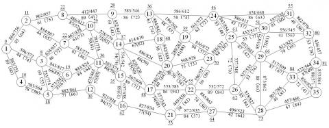
In the existing multimodal transport network, as shown in Figure 4, a batch of goods is transported from node 1 to node 35. The length of each segment is represented by km (railway /road distance), and its maximum transport capacity is t (railway / highway capacity). At each node, the departure time specified on the railway is represented by h (DT). To simply the calculation, the DT at each node is calculated according to the accumulated time [16].
Figure 4. Conjunction of urban nodes
Table 1. Features of transport modes
|
Transport Mode |
Average speed (km/h) |
Transportation quantity charge (t) |
Freight charge (yuan/t.km) |
Transfer cost (yuan/t) |
|
Railway |
80 |
(0,20] (20,40] (40,60] |
0.18 0.25 0.29 |
10 |
|
Highway |
90 |
(0,10] (10,30] (30,60] |
0.24 0.33 0.37 |
4.2 Algorithm test
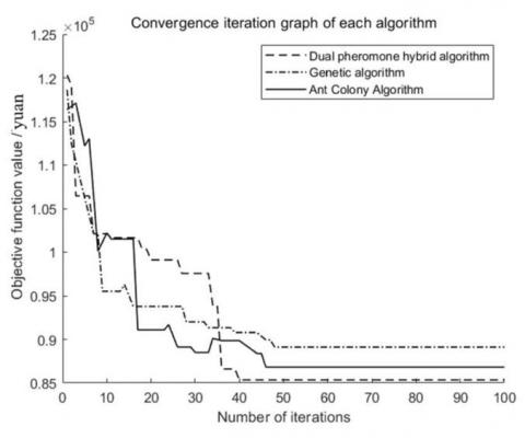
According to the above algorithm, the relevant parameters set herein are listed in Table 2. Since both the GA and the ACO belong to the heuristic algorithm that has convergence result with certain randomness. The algorithm runs 10 times to take the best solution and performance evaluation indices for comparison. The best results of each algorithm are shown in Table 3. The comparison in the iterative convergence between them is shown in Figure 5.
By comparison, it is known that the average convergence iterations of dual pheromone hybrid algorithm proposed herein can be 20.08% and 17.49% lower than those of single GA and the ACO, respectively, and the average fitness function by 4.23% and 2.39%, respectively, under the constant conditions, which shows that this algorithm has a faster convergence and better optimization performance, so is efficient and feasible in practical transportation operations.
Table 2. Initial values of algorithms
|
Parameters |
Symbol |
Initial value |
|
Number of nodes |
c |
35 |
|
Population size |
m |
100 |
|
Crossing rate |
Pc0 |
0.8 |
|
Variability rate |
Pm0 |
0.2 |
|
Max generations |
g |
20 |
|
Number of ants |
n |
50 |
|
Pheromone factors |
α |
1 |
|
Priori factors |
β |
3 |
|
Volatile factors |
ρ |
0.1 |
|
Cycle number of hybrid algorithm |
G |
100 |
|
Freight volume |
q |
50 |
|
Delivery time limit |
[Tke,Tkl] |
[72,84] |
Table 3. Solutions of algorithms
|
Algorithm |
Best route |
Best transport mode |
Benefit (yuan) |
Time (h) |
Average Convergence Algebra |
|
Hybrid Algorithm |
1→2→8→9→13→24→30→32→34→35 |
R→R→R→R→R→H→H→R→R |
85347 |
77.751 |
38.2 |
|
GA |
1→4→5→12→16→21→27→28→35 |
R→R→R→R→R→R→H→H |
89112 |
80.681 |
47.8 |
|
ACO |
1→2→7→11→15→17→22→27→28→35 |
R→R→R→R→R→R→R→H→H |
86816 |
82.546 |
46.3 |
Figure 5. Convergence iteration of algorithms
4.3 Case analysis
To further test how the final path selection is subject to relevant conditions in the model and whether the proposed algorithm is effective, the paper analyzes the capacity limits, the arrival time limit and the transportation cost, respectively, see below for details:
(1) Given how the sensitivity of goods is to the time limits, that is, change the arrival time limit of the goods, find the solution using the hybrid algorithm, as shown in Table 4, the algorithm iteration is shown in Figure 6;
Figure 6. Convergence iteration when arrival time limits change
Table 4. Solution of hybrid algorithm when arrival time limits change
|
Delivery time limit |
Best route |
Best transport mode |
Benefit (yuan) |
Time (h) |
Average Convergence Algebra |
|
[60,72] |
1→3→7→11→15→17→21→27→28→35 |
R→R→R→R→R→R→R→H→H |
76776 |
72.942 |
31.3 |
|
[72,84] |
1→2→8→9→13→24→30→32→34→35 |
R→R→R→R→R→H→H→R→R |
85347 |
77.751 |
38.2 |
|
[84,96] |
1→2→8→9→13→19→24→30→32→34→35 |
R→R→R→R→R→R→H→H→R→R |
87725 |
88.380 |
32.8 |
(2) Given that the capacity of certain segment decreases due to congestion or the like, for example, the departure at the node 2 is restricted, or the path capacity increases due to the rebuilding and expansion (it is true for the network capacity), the solutions of hybrid algorithm are listed in Table 5. The algorithm iteration is shown in Figure 7;
Table 5. Solutions of hybrid algorithm when path capacity limits change
|
Capacity constraints |
Best route |
Best transport mode |
Benefit (yuan) |
Time(h) |
Average Convergence Algebra |
|
Decreased capacity |
1→4→5→12→16→21→27→28→35 |
R→R→R→R→R→R→H→H |
89122 |
80.238 |
37.4 |
|
Normal capacity |
1→2→8→9→13→24→30→32→34→35 |
R→R→R→R→R→H→H→R→R |
85347 |
77.751 |
38.2 |
|
Increased capacity |
1→3→7→11→15→17→21→27→28→35 |
R→R→R→R→R→R→R→R→R |
71630 |
82.561 |
33.6 |
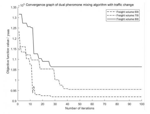
Table 6. Solution of dual pheromone hybrid algorithm when traffic volume changes
|
Freight volume(t) |
Best route |
Best transport mode |
Benefit (yuan) |
Time (h) |
Average Convergence Algebra |
|
60 |
1→4→5→12→16→21→27→28→35 |
R→R→R→R→R→R→H→H |
89122 |
80.649 |
29.6 |
|
70 |
1→2→8→9→13→24→25→26→28→35 |
R→H→R→R→H→R→R→R→H |
95514 |
79.498 |
42.3 |
|
80 |
1→4→5→6→11→15→17→22→26→28→35 |
R→R→R→R→R→R→H→H→H→H |
106375 |
89.262 |
28.9 |
Figure 7. Convergence iterations of algorithms when there is no capacity limit
Figure 8. Convergence of dual pheromone hybrid algorithm when traffic volume changes
(3) Given that the shipper and the carrier sign a long-term contract under which the quantity is constant, that is, the average cost instead of the segment cost is used for calculation. For different traffic volumes, the hybrid algorithm finds the solution, as shown in Table 6. The algorithm iteration convergence is shown in Figure 8.
By comparison, it is found that the model mentioned herein is feasible, and the finally selected path is inseparable from capacity limit, the arrival time limit and the transportation cost. The proposed algorithm is effective and can converge quickly.
(1) The combined optimization model is established to minimize the transport cost, considering the "scale effect" of the transport economy, based on the practical operation of multimodal transport and customer demand, and with a constant piecewise linear function as the transport cost.
(2) In view of the good global search capacity of genetic algorithm in early stage and the strong convergence of positive and negative feedback in the late stage of the ACO, the dual pheromone hybrid algorithm is designed with the solutions of rapid convergence.
(3) To avoid the hybrid algorithm trapping in the local optimal solution, the dynamic genetic operator is designed in the genetic algorithm; the adaptive catastrophe factor is introduced in the ant colony optimization process, and the jump operation is randomly selected to improve the global optimization capacity of algorithm based on the population diversity.
(4) The feasibility and efficiency of the algorithm is further tested with a case, and the different results of path selection under different constraints are discussed in detail.
(5) The assumptions are made on the transshipment process hereof. The model does not describe the practical transshipment process in detail. When the transshipment cost and constraints change greatly, it should be further improved.
The work described in this paper was fully supported by: Youth Science Foundation of Lanzhou Jiaotong University (No. 2018018); National Natural Science Foundation of China (No.71671079); The Humanities and Social Science Foundation of Ministry of Education of China (No.15YJCZH10). Lanzhou Bureau Group Corporation's Science and Technology Development Project in 2019 (No. KY201979).
[1] Reddy, V.R., Kasilingman, R.G. (1995). Intermodal transportation considering transfer costs. Proceedings of the 1995 Global Trends Conference of Academy of business Administration.
[2] Moccia, L., Cordeau, J.F., Laporte, G., Ropke, S., Valentini, M.P. (2011). Modeling and solving a multimodal transportation problem with flexible-time and scheduled services. Networks, 57(1): 53-68. https://doi.org/10.1002/net.20383
[3] GrBener, T. Berro, A., Duthen, Y. (2010). Time dependent multiobjective best path for multimodal urban routing. Electronic Notes in Discrete Mathematics, 36: 487-494. https://doi.org/10.1016/j.endm.2010.05.062
[4] Zhang, J., Zhang, Q., Zhang, L. (2015). A study on the paths choice of intermodal transport based on reliability. Berlin Heidelberg: Springer. https://doi.org/10.1007/978-3-662-43871-8_46
[5] Rekik, M., Mellouli, S. (2011). A reputation-based winner determination problem for combinatorial transportation procurement auctions. Journal of the Operational Research Society, 63(10): 1400-1409. https://doi.org/10.1057/jors.2011.108
[6] Wang, H., Wang, C.X. (2012). Selection of container types and transport modes for container multi-modal transport with fuzzy demand. Journal of Highway and Transportation Research and Development, 29(4): 153-158. https://doi.org/10.3969/j.issn.1002-0268.2012.04.027
[7] Jiang, J., Zhang, P. (2014). Route optimization of unban waterlogging rescue based on improved ant colony optimization. Journal of Computer applications, 34(7): 2103-2106. https://doi.org/10.11772/j.issn.1001-9081.2014.07.2103
[8] Wan, J., Wei, S. (2019). Multi-objective multimodal transportation path selection based on hybrid algorithm. Journal of Tianjin University, 52(3): 285-292. https://doi.org/10.11784/tdxbz201807034
[9] Liu, J., Peng, Q., Yin, Y. (2018). Multimodal transportation route planning under low carbon emissions background. Journal of Transportation Systems Engineering and Information Technology, 18(6): 243-249.
[10] Liang, X. (2017). A study on optimizing routes of railway containerization mulimodel transport with fuzzy time constraints. Railway Transport and Economy, 39(12): 55-60.
[11] Mitsuo, G. (2017) Network models and multiobjective genetic algorithm. Beijing: Tsinghua University Press.
[12] Wang, Y., Jia, J. (2014). Joint transportation path optimization based on hybrid algorithm. Journal of Transport Information and Safety, 32(1): 64-67.
[13] Duan, H. (2005). Ant colony algorithms: Theory and applications. Beijing: Science Press.
[14] Lim, A., Xu, R. (2008). Transportation procurement with seasonally varying shipper demand and volume guarantees. Operations Research, 56(3): 758-771. https://doi.org/10.1287/opre.1070.0481
[15] Tang, J., Li, X. (2008). Organizing optimization model and its algorithm of container multimodal transportation. Journal of Transport Information and Safety, 3: 89-91. https://doi.org/10.1061/9780784412602.0008
[16] Xiong, G., Wang, Y. (2011). Optimization algorithm of multimodal transportation with time window and job integration of multiagent. Journal of Systems Engineering, 26(3): 379-386.