Jun Pan| Zuo Fu | Hongwei Chen*
OPEN ACCESS
In the classic split delivery vehicle routing problem, the demands of customers can be split unconditionally into pieces of any size. However, in the real-world distribution system, the customer demands consist of a set of orders on different quantities of goods. During the distribution, demands can be spitted, but orders cannot. This paper considers the vehicle routing problem with split delivery by order. It formulates the problem as an integer linear programming model, creatively applies the binary to the decimal decoder method to represent the solution, proposes a heuristic order-insertion procedure, and develops a tabu search algorithm. Using the developed algorithm, this paper tests 25 benchmark instances. According to the test results, the algorithm proposed has a small gap with the best-known solutions, but has an advantage in computing time.
vehicle routing, discrete split delivery, ejection chains, tabu search
The vehicle routing problem (VRP) is the core of logistics and transportation. In this problem, a fleet of homogenous vehicles are used to serve a set of customers, and each customer is visited by a single vehicle, and the objective is to minimize the total transportation cost. The split delivery routing problem (SDVRP) relaxes the restriction that each customer is visited only once; in other words, a customer is allowed to be visited by more than one vehicle. With the split delivery allowed, both the traversal distance and the number of vehicles are desired to be reduced.
In the classic SDVRP, the customer demands can be spitted into pieces of any size unconditionally. However, in the real-world urban logistics distribution system, distribution centres provide daily services for B2B and commodity customers in urban areas. The customer demands consist of a set of orders, each of which has a different quantity of goods. The demands can be split, but the order cannot. Therefore, it is necessary to further study the VRP with split delivery by order.
Figure 1 illustrates an example of the DSDVRP with three customers and a depot, where the edge labels indicate distances and the node labels in parentheses are the customer demands. The vehicle capacity is 100. Figure 1(a) shows the optimal solution to the classical VRP, which contains three direct trips for each customer, and the total distance is 60. With split delivery allowed, customer 2 is visited by two vehicles (Figure 1(b)). Consequently, the total traversal distance drops to 52, and 2 routes are involved. In Figure 1(c), a vector is used to denote the customers’ demands. The dimensions of the vector represent the number of orders and the component represents the quantity of each order. Because customer 2 and customer 1 have only one order each, their demands cannot be split. Hence, the solution in Figure 1(b) is infeasible for the DSDVRP. Figure 1(c) shows the optimal solution to the DSDVRP where the demand of customer 3 is split by order. The total distance (i.e. 56) is larger than that of the SDVRP. In conclusion, if the quantity of each order is 1, the DSDVRP is equivalent to the SDVRP; in other words, the DSDVRP is a generalization of the SDVRP.
VRP
SDVRP
DSDVRP
Figure 1. Comparison of the VRP, SDVRP and DSDVRP
Nakao et al. [1] first defined the problem as the discrete split delivery vehicle routing problem (DSDVRP) and proposed a heuristic algorithm based on dynamic programming. The algorithm was tested in real-world instances of a huge manufacturer, and exhibited efficient performance. Salani et al. [2] considered the DSDVRP with time windows and developed a branch-and-price algorithm. Z. Fu et al. [3] studied with the DSDVRP with soft time windows and proposed a tabu search algorithm. All these algorithms mentioned above took orders as operation objects. There are also other researchers who adopted prior split strategies. M. Qiu [4] aggregated randomly some orders of each customer into a new order in advance, and then transferred the DSDVRP into the classic capacitated vehicle routing problem (CVRP). Chen et al. [5] also proposed two prior split rules called 25/10/5/1 or 20/10/5/1 for the SDVRP. The approach of considering orders as independent customers can multiply the scale of the DSDVRP and make it difficult to solve.
This paper proposes a new tabu search algorithm, which takes customers as operation objects. The remainder of the paper is organized as follows. This research is based on the theory of SDVRP, so it reviews the literatures on the SDVRP in section 2. In section 3, it formulates a mathematic model for the DSDVRP and analyzes the properties of optimal solutions. In section 4, it develops a tabu search algorithm for solving the DSDVRP. In section 5, it presents the computational results. Finally, this paper is concluded in section 6.
The primary motivation to split the customer demands is to reduce the traversal cost and the number of vehicles. Dror and Trudeau [6] showed that allowing split delivery can save costs. Archetti et al. [7] proved that the traversal cost saving that can be obtained is at most 50 % and that this bound is tight. These authors also studied the properties of optimal solutions. Dror and Trudeau [6] proved that the SDVRP is NP-hard. If the traversal cost satisfies the triangle inequalities, there exists no optimal solution where two routes can cover more than one customer (such a configuration is called a 2-split cycle). Archetti et al. [7] derived another property of the optimal solution: the number of splits is smaller than that of the routes if the distance cost satisfies the triangle inequalities.
Considering that the SDVRP is NP-hard, a variety of heuristic procedures for the SDVRP have been proposed. Dror and Trudeau [6] first developed a local search algorithm, which incorporated k-split interchanges and route additions. Archetti et al. [8] presented a tabu search algorithm called SPLITABU, which uses two procedures called ORDER ROUTES and BEST NEIGHBOUR. With only two parameters, SPLITABU is very easy to implement, and the variants of SPLITABU can provide high quality results. Chen et al. [9] combined a mixed integer program and a variable-length record-to-record travel algorithm into a new method for the SDVRP. The hybrid algorithm outperformed the tabu search algorithm proposed by Archetti et al. in solving six test problems with 50~199 customers and again performed well in solving other five problems where lower bounds exist. In the last decade, Silva. et al. [10] proposed an iterated local search heuristic algorithm, which is highly competitive.
Several researchers also focused on the exact solution methods. Belenguer, Martinez and Mota [11] studied the polyhedron of the SDVRP and found new valid inequalities that define facets through a cutting plane algorithm in conjunction with a relaxed formulation. The gaps between the lower and upper bounds are within 12% for problems with 50, 75, and 100 customers. Lee et al. [12] modelled a dynamic programming model of the SDVRP, which is able to solve test problems with up to 7 customers. Jin et al. [13] developed a two-stage algorithm which divides the SDVRP into two sub-problems: the first is an assignment problem that determines the clusters of customers served by the same vehicle, and the second is a TSP for each cluster. The algorithm can solve test problems with up to 22 customers. Arichetti et al. [14] proposed a column generation algorithm that solves the test problems with up to 100 customers.
Moreover, several variants of the SDVRP have been studied for both theoretical and practical purposes. Gulczynski et al. [15] considered the SDVRP with an additional constraint: each customer has a minimum delivery amount, which is defined as a fixed fraction of the demand. Jia Fu et al. [16] studied the split-delivery weighted vehicle routing problem, which takes the cargo weight into account. Zuo Fu [3] studied the vehicle routing problem with soft time windows and split delivery by order in the context of pure distribution with a single depot and a heterogeneous fleet of vehicles.
The DSDVRP is defined on a complete graph G=(N,E), where N={0,1,...,n} is the set of nodes and E is the set of edges. Node 0 denotes the depot, and the others represent the n customers. A distance matrix $C=(c_{ij} )$ is defined on the set E, each element of which denotes the distance between node i and node j. Let $n_i$ stand for the number of customer i’s orders, and $d_i^k (k=1,⋯,n_i)$ denote the demand of the customer i’s k-th order. The total demand of customer i is $d_i$, which is equal to the sum of $d_i^k (k=1,⋯,n_i)$, i.e. $d_i=d_i^1+d_i^2⋯+d_i^{n_i}.$.
We assume the following:
●Each route begins and ends at the depot;
●The number of vehicles m is unlimited;
●Each of the vehicles is homogeneous with a capacity of Q;
●The customers’ demands can be split, but the orders cannot.
$x_{ijl}$ is a binary variable, which is 1 if vehicle l travels from customer i to customer j, and 0 otherwise. $ y_{ikl}$ is another binary variable, which equals to 1 if vehicle l delivers customer i’s k-th order, and 0 otherwise. The DSDVRP can be modelled as follows.
$min\sum_{i=0}^n\quad \sum_{j=0}^n\quad \sum_{l=1}^m\quad c_{ij}x_{ijl}$ (1)
s.t. $\sum_{i=0}^n\quad \sum_{l=1}^m\quad x_{ijl}≥1 j=0,...,n$ (2)
$\sum_{j=1}^n\quad x_{ijk}=\sum_{j=1}^n\quad x_{jik} i=0,...,n; k=1, .., m$ (3)
$\sum_{i∈S}\quad\sum_{j∈S}\quad x_{ij}≤|S|-1 k=1,...,m; S⊆N$ (4)
$\sum_{k=1}^{n_i}\quad \sum_{l=1}^m\quad d_{ik}y_{ikl}=d_i i=1,...,n$ (5)
$\sum_{i=1}^n\quad \sum_{k=1}^{n_i}\quad d_{ik}y_{ikl}≤Q, l=1,...,m$ (6)
$y_{ikl}≤\sum_{j=1}^n\quad x_{ijl} i=1,...,n,k=1,...,n_i,l=1,...,m$ (7)
$x_{ijk}∈\lbrace 0,1\rbrace i=0,...,n j=0,...,n;k=1,...,m$ (8)
Formula (1) is the objective function, targeting the minimum traversal distance of vehicles. Constraint (2) mean that each customer is visited by one vehicle at least; constraint (3) imposes the equilibrium condition of goods flow; constraint (4) is the classic sub-tour elimination constraint; constraint (5) ensures the total demand of customers can be satisfied; constraint (6) requires that the delivery amount of each vehicle should not exceed its capacity; and constraint (7) imposes the connectivity of the route performed by l.
As mentioned in section 2, Dror and Trudeau [6] proved that if the distance satisfies the triangle inequalities, the optimal solution to the SDVRP does not contain any k-split cycle ($k≥2$), which means there is at most one node between any two routes in the optimal solution to the SDVRP. However, this result does not hold for the DSDVRP. Figure 2 illustrates the case. In this example, there are three customers with two orders per customer. The capacity of each vehicle is 100, and the total demand of all the customers is 200, so the optimal solution needs at least two vehicles. First the solution with three direct trips from each customer to the depot has a total traversal distance of 60. Next, it is clear that no pair of customers can be visited in one route without violating the vehicle capacity. Further, consider the route visiting each customer. The routes of this solution are: 0-1(55)-2(15)-3(30)-0, 0-1(30)-2(50)-3(20)-0, where the integers in parenthesis are the demands delivered by vehicles, and the total distance is 44. Then, this solution is optimal, in which each two of the customers constitute a 2-split cycle. The example indicates that the structure of the optimal solution to the DSDVRP may be more complex than that for the SDVRP.
Figure 2. In the example, the optimal solution has a 2-split cycle
Since it was developed by Glover in 1988, Tabu Search (TS) has been standing out as the best metaheuristic for a variety of VRPs. Similar to the Hill-climbing algorithm, TS explores the solution space by moving from the current solution $x_k$, at iteration k, to its best neighbour $x_{k=1}$ in the neighbourhood $N(x_k)$. To avoid cycling, TS uses the tabu list to record some attributes of the recently examined solutions, and moves in the tabu list are forbidden unless their neighbourhood solution satisfies the aspiration criterion. To escape from the local optimal solution, several implementations can be adopted, such as intermediate infeasible solutions, intensification and diversification strategies.
In this section, a new tabu search algorithm is presented, which takes customers as operation objects and uses embedded neighbourhood structures based on ejection chains. To accelerate neighbourhood search, the Neighbour Route of each customer is defined (see definition 1) to reduce the solution neighbourhood cardinality. The Neighbour Route will be dynamically adjusted during the search process. Of course, it may get too strong and forbid high-quality neighbourhood solutions. For this reason, the perturbation mechanism is used after a given number of non-improving iterations.
Definition 1 If route r contains at least one of the p customers nearest to customer i, r is the Neighbour Route of customer i. The set of neighbour routes of customer i is denoted by $NR_i$.
4.1 Representation and decoding method
In the papers by Nakao et al. [1], M. Qiu et al [4] and F. Zuo [2], the different orders of the same customer were dealt with as independent customers, and the solution was represented by a sequence of orders. In this section, a new coding method is proposed, which is called the Binary to Decimal Decoder method (BDD), to represent solutions of the DSDVRP. For example, there is a route represented by an integer string 0-3(5)-4(3)-6(2)-8(7)-11(5)-0. The integer string outside the parentheses represents the service sequence in the route. By converting decimal integers in parentheses to binary numbers, we can get the message of the orders delivered in the route. For example, integer 5 decoded to binary numbers is equal to 101. From right to left, 101 means only the first and third orders of the corresponding customer are delivered in the route. Figure 3 shows a route string which can be decoded by BDD.
Figure 3. Solution representation
4.2 Initial solution
The initial solution is generated by an insertion-based algorithm. The insertion of orders can be modelled as the knapsack problem, which can be solved by the dynamic programming based algorithm. However, Boudia et al. [18] pointed out the dynamic programming cannot significantly improve the solution found by the greedy heuristic. For the sake of computing time, this paper applies the simple greedy heuristic in which insertions are performed by the decreasing order of $d_i^j$. Furthermore, customer node i is permitted to be inserted into route r only if the sparse capacity of route r is no less than the minimum unrouted order of customer i. Algorithm 1 shows the pseudocode of inserting customer $i^{'} s$ unrouted orders into an unforbidden route $r_k$.
Notation:
L: the list of unrouted customers;
$s_r$: the sparse capacity of route r;
$q_{ir}$: the delivery amount of customer i served by route r;
$U_i$: the set of unrouted orders of customer i.
Table 1. Pseudocode of inserting i into $r_k$
|
Algorithm 1 insert customer $i^{'} s$ unrouted orders into an unforbidden route $r_k$ |
|
|
1: |
Procedure IOR( $U_i$, $p_k$); |
|
2: |
$U_i \gets$ the list of the unrouted orders of customer i, and the orders are sorted by decreasing order; |
|
3: |
$q_{ir} \gets 0$; |
|
4: |
while $p_k≥min{d_i^j|d_i^j∈U_i}$ do; |
|
5: |
for each $d_i^j$ in $U_i$ do; |
|
6: |
if $d_i^j ≤ p_k$ ; |
|
7: |
$U_i \gets U_i \backslash \lbrace d_i^j\rbrace$; |
|
8: |
$s_k \gets s_k-d_i^j$; |
|
9: |
$q_ir \gets q_ir+d_i^j$; |
|
10: |
return $U_i$ and $p_k$ and $q_ir$ |
Table 2. Pseudocode of constructing the initial solution
|
Algorithm 2 construct the initial solution |
|
|
1: |
Procedure initial construction |
|
2: |
initial $R\gets ϕ$, $L\gets $ the list of unrouted customers, $k\gets 1$; |
|
3: |
for each i in L do |
|
4: |
$U_i \gets$ the set of unrouted order of i, in which orders are sorted by decreasing order of $d_i^j$; |
|
5: |
$t \gets argmax_{i∈L}\backslash \lbrace c_{i0}\rbrace$; |
|
6: |
$r_k \gets (0-t-0)$, $R \gets R∪\lbrace r_k\rbrace$, $s_k \gets Q-d_i$, $q_{ik} \gets d_i$; |
|
7: |
update $L \gets L\backslash\lbrace t\rbrace$; |
|
8: |
while $L≠ϕ$ do |
|
9: |
for each i in L do |
|
10: |
$ε^* \gets ∞$, $τ^*\gets ∞$; |
|
11: |
for each r in R do |
|
12: |
if $s_k≥min\lbrace d_i^j│d_i^j∈U_i \rbrace$ |
|
13: |
$ε_{ir}\gets$ the cheapest cost of inserting i into r; |
|
14: |
if $ε_{ir}<ε^*$ |
|
15: |
$ε^*\gets ε_{ir}$, $r^*\gets r_i$, $i^*\gets i$; |
|
16: |
$τ^*\gets μc_{0i}-ε_{ir_i }$; |
|
17: |
if $τ^*<0$ |
|
18: |
$r^*\gets$ insert i in the position with the lowest cost of $r^*$; |
|
19: |
$(U_{i^* }, p_{r^* },q_{i^*,r^*}$ IOR($U_{i^* }, p_{r^* }$); |
|
20: |
else |
|
21: |
$k\gets k+1$, $r_k\gets (0-i^*-0)$; |
|
22: |
$R\gets R∪\lbrace r_k\rbrace$, $s_k\gets Q-\sum_{d_{i^*}^j} ∈U_{i^* }, d_{i^*}^j$, $q_{ik}\gets \sum_{d_{i^*}^j} ∈U_{i^* }, d_{i^*}^j$; |
|
23: |
If $U_i=∅$ |
|
24: |
$L\gets L\backslash\lbrace i^*\rbrace$; |
|
25: |
return R |
This paper develops a parallel insertion heuristic to construct the initial solution to the DSDVRP. The routes are expanded under the two constructions:
$ε_{ir}=(c_{si}+c_{it}-λc_{st})$ (9)
$τ_{ir}=2c_{0i}-ε_{ir}$ (10)
where $ε_{ir}$ is the lowest generalized cost of inserting customer i into route r; and s and t are the preceding and succeeding customers, respectively, in route r after customer I is inserted; $λ$ is a route shape parameter proposed by Gaskell [19] and Yellow [20] to improve the initial solution; $τ_{ir}$ is a discriminant function to decide whether to insert i into route r or create a new route with i. The pseudocode of constructing the initial solution is summarized in Table 2. L is the list of unrouted customers, and the first route $r_1$ is constructed with the farthest unrouted customer node from the depot (line 5-7). Then the procedure continues to select the insertion candidate (line 9-16). If $τ^*<0$, create a new route with the corrosponding customer node, or otherwise insert the node into the related route (line 17-22). Update the unrouted customer list L (line 23-24). Repeat the process until L is empty.
4.3 Neighbourhood structure
The neighbourhood structure is an important aspect of Tabu search applications, where a set of moves are defined to transit a current solution into a new one. In order to enhance the ability of global searching and prevent early convergence, researchers apply a mixed neighbourhood structure that usually consists of node-shift or arc-exchange operators. At each iteration, a move is achieved by selecting a random one or the best of all neighbourhood structures.
Ejection chain is an innovative neighbourhood structure defined by Glover [21]. An ejection chain can be viewed as a series of triplets, each consisting of three consecutive nodes in a route. And the neighbourhood solution is obtained by moving a node to the position occupied by another. As a result, the ejection chain procedure provides a way of compressing a sequence of moves into a compound move. Inspired by the idea, Rego and Roucairol [22] proposed a tabu search for the VRP, and A. Fu et al. [23] developed a highly adaptive neighbourhood structure, called the split-delivery node ejection chain (SNEC), for the split delivery vehicle routing problem with the minimum delivery amount. In this section, the SNEC is modified in the tabu search phase. The operator denoted by SNEC* starts with ejecting customer node i from route $r_s$ to an adjacent route $r_t$. If the sparse capacity $r_t$ is enough, locate i in the position of $r_s$ with the lowest cost. Otherwise, transfer some or the entire delivery amount of a different customer j in route $r_t$ to another route $r_l$. The operator involves the following three types of neighbourhood structures.
Type I: relocation. For customer node $i∈r_s$ and $r_t∈NR_i$, remove customer node i to the position with the lowest cost in $r_t$. If i is split between $r_s$ and $r_t$, delete the split. This move is feasible when $s_i≥q_{ir_i }$.
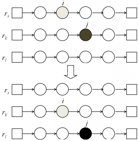
Type II: ejection chain. Type II is illustrated in Figure 4. For customer node $i∈r_s$ and route $ r_t∈NR_i$, remove customer node i to the position with the lowest cost in $r_t$. If route $r_t$ is overloaded, remove customer node $j∈r_t (j≠i)$ to the position with the lowest cost in $r_l∈NR_j$. This move is feasible when $r_l$ has sufficient sparse capacity to serve j. If $r_l=r_s$ , the move is similar to the classic 1-1 exchange.
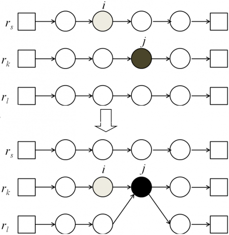
Type III: new split. Type III is illustrated in Figure 5. For customer node $i∈r_s$ and route $r_t∈NR_i$, remove customer node i to the position with the lowest cost in $r_t$. If route $r_t$ is overloaded, shift some orders of customer $j∈r_t (j≠i)$ to the position with the lowest cost in $r_l∈NR_i$. In this case, the demand of customer node j is split between $r_t$ and $r_l$. The move is feasible when the shifting demand of j can cover the lack of capacity $r_s$. The insertion of customer node j into $r_l$ applies IOR.
Figure 4. Illustration of Type II
Figure 5. Illustration of Type III
Once the neighbourhood is triggered by customer node i, the reaction of the subsequent process depends on the total saving cost. In other words, the nodes, routes and delivery amounts of the subsequent process will be selected adaptively, leading to the maximum cost saving.
4.4 Perturbation mechanism
To escape the local optimal solution, this paper applies strategic perturbation to diversify the local search region. The pseudocode of the perturbation procedure is demonstrated in Table 3. The perturbation mechanism consists of a destroy operator and a repair operator. The destroy operator first selects q customer nodes at random and then removes them from all their routes (line 2-3). The destroy operator plays a role in diversifying the solution space. The repair operator reinserts the selected customer nodes into routes (line 8-18).
Table 3. Pseudocode of perturbating the current solution
|
Algorithm 3 perturbate the current solution |
|
|
1: |
Procedure perturbation(R) |
|
2: |
L¬the list of the q unrouted customers selected at random |
|
3: |
S¬remove the customer nodes in L from S |
|
4: |
for each i in L do |
|
5: |
$U_i\gets$the list of the unrouted orders of customer i, and the orders are sorted by decreasing order |
|
6: |
while $L≠ϕ$ do |
|
7: |
$I^*\gets∞$; |
|
8: |
for each i in L do |
|
9: |
for each $r_k$ in R do |
|
10: |
if $s_k≥min\lbrace d_i^j│d_i^j∈U_i \rbrace$ |
|
11: |
$I_{ik}gets$ the cheapest cost of insert i into $r_k$ |
|
12: |
if $I_{ik}< I^*$ |
|
13: |
$I^*\gets I_{ik} i^*\gets i k^*\gets r_k$; |
|
14: |
if $I^*<∞$ |
|
15: |
R $\gets$ insert $I^*$ into $r_{k^* }$; |
|
16: |
else |
|
17: |
$I^*\gets$ select a customer in L at random; |
|
18: |
R $\gets R∪\lbrace (0,I^*,0)\rbrace$ |
|
19: |
update $U_i$; |
|
20: |
If $U_{i^* }=Φ$ |
|
21: |
$L=L\backslash\lbrace i^* \rbrace$ |
|
22: |
return R |
4.5 Framework of tabu search
The proposed solution algorithm is a three-phased tabu search algorithm. It starts with the initial solution by the initial construction procedure. The tabu search phase adopts the adaptive neighbourhood structure SNEC*. At each iteration, the solution is associated with the attributes (i,j). The inverse ejection (j,i) should be forbidden for $θ$ iterations. The value of $θ$ depends on the number of customers and the number of routes. Practical experiments indicate that changing the value at random is more effective than setting a fixed number. So the value of $θ$ is chosen randomly within the interval $[θ_{min},θ_{max}]$ during the search. Nevertheless, the tabu status of an attribute can be revoked if the move improves $s^*$ (the best solution found so far). The aspiration criteria are defined as $f(s)<f(s^*)$. If $s^*$ is not improved during successive iterations, the perturbation procedure will be called for diversifying the searching space. At last, every route in $s^*$ is re-optimized by the 3-opt procedure. Table 4 shows the framework of the tabu search.
Table 4. Framework of the tabu search
|
Algorithm 4 Tabu search |
|
|
1: |
$s\gets$ initial construction |
|
2: |
$s^*\gets s f^*\gets f(s)$; |
|
3: |
counter $\gets 0$ ; |
|
4: |
while counter <maxIters do |
|
5: |
s$\gets$ {SNEC*(s)| s subject to tabu and aspiration conditions}; |
|
6: |
If $f(s)< f(s^*)$ |
|
7: |
$s^*\gets s f(s^*)\gets f(s)$ |
|
8: |
counter $\gets 0$ |
|
9: |
else counter $\gets$counter+1 |
|
10: |
If counter >perIter |
|
11: |
s $\gets$ perturbation(s) |
|
12: |
$s^*\gets$ post optimize $s^*$ by the 3-opt procedure; |
|
13: |
return $s^*$ |
The DSDVRP is new in literatures, so there is no benchmark instance yet, and what is more, the most related instances used by Nakao et al. are also unavailable. This paper uses the test instances generated from the TSPLIB and those proposed by Chen et al. [9]. For each customer, orders are generated by the prior split strategy called 20/10/5/1 rule or 25/10/5/1 rule. For details of the rules, please refer to Chen et al. [9]’s paper. The number of customers ranges from 21 to 100, and the number of orders from 66 to 590. The algorithm proposed here is coded in Matlab R2014 a and implemented on a personal computer with a 2.40 GHz, i5-2430 processor, 4GB of RAM and the Windows 7 operating system.
5.1 Algorithm calibration
The algorithm proposed in this paper has 7 parameters to set: 1) the route shape parameter (λ) ; 2) the p nearest customer nodes (p); 3) the q customer nodes selected randomly for perturbation (q); 4) the tabu list size (θ); 5) the perturbation cycle (perIter); 6) the maximum iterations (maxIter); and 7) the candidate list size (m). In the initial construction phase, the customer nodes far from the depot are given priority to be inserted into a route. If the generalized cost of inserting i to r is greater than the cost of creating a new directed route, the initial construction will create the route (0-i-0). So λ is chosen within the interval [0.7, 1]. To calibrate the parameter p, sensitivity analysis is performed on all the test instances, and the test results indicate the sensitivity interval of p is [8,10]. θ is a random integer in the interval [5, 20]. In the perturbation phase, q is chosen randomly among 5, 6 or 7. The perIter is equal to 10. According to the experiment, the maxIter is fixed at 10n, and the candidate list size m at n.
5.2 Test results
Table 5 and 6 present the test results of set 1 and set 2, respectively, in which the fifth and sixth columns are the cost and computing time of the proposed algorithm. After comparison with the results provided by the tabu search algorithm developed by M. Qiu. [3], it is found that the proposed algorithm outperforms the former in 12 instances and equals it in 2 instances among all the 25 instances, as shown in Table 5. Table 6 shows that the proposed algorithm has better performance in 14 instances and equal performance in 5 instances. From the two tables, it can be seen that some results yield slightly different costs with the results provided by M. Qiu. [3] due to the rounding errors in the cost data. The computational results indicate that the proposed sub-algorithms of IOR and SENC* can better reflect the features of the discrete split and diversify the search space of the solution in contrast to the prior split strategy.
Table 5. Results for set 1
|
Instance (20/10/5/1) |
Order quality |
TS |
TS |
||
|
Cost |
Time(b) (Seconds) |
Cost |
Time(c) (Seconds) |
||
|
eil22 |
66 |
375.28 |
9.38 |
375.8 |
1.54 |
|
eil23 |
73 |
568.56 |
19.93 |
568.56 |
1.67 |
|
eil30 |
108 |
512.72 |
33.81 |
498.02 |
2.68 |
|
eil33 |
108 |
837.67 |
43.75 |
837.06 |
3.56 |
|
eil51 |
188 |
524.61 |
54.63 |
524.61 |
12.5 |
|
eilA76 |
284 |
860.11 |
80.42 |
849.61 |
97.8 |
|
eilB76 |
256 |
1037.93 |
169.64 |
1034.21 |
120.9 |
|
eilC76 |
262 |
745.92 |
106.3 |
746.79 |
39.16 |
|
eilD76 |
268 |
719.05 |
203.05 |
687.6 |
120.45 |
|
eilA101 |
346 |
824.09 |
351.64 |
826.14 |
217.89 |
|
eilB101 |
413 |
1098.95 |
402.41 |
1099.34 |
311.25 |
|
SD51D1 |
179 |
457.67 |
32.3 |
459.5 |
12.25 |
|
SD51D2 |
205 |
714.05 |
62.31 |
718.69 |
36.58 |
|
SD51D3 |
239 |
971.46 |
62.12 |
965.13 |
55.63 |
|
SD51D4 |
306 |
1624.55 |
180.11 |
1645.91 |
43.12 |
|
SD51D5 |
296 |
1392.15 |
203.44 |
1387.19 |
44.51 |
|
SD51D6 |
374 |
2360.93 |
230.77 |
2273.51 |
77.82 |
|
SD76D1 |
267 |
600.19 |
44.97 |
601.43 |
15.32 |
|
SD76D2 |
329 |
1413.73 |
147.32 |
1226.5 |
90.12 |
|
SD76D3 |
377 |
1702.57 |
207.87 |
1546.33 |
116.34 |
|
SD76D4 |
427 |
2171.96 |
357.99 |
2179.1 |
213.03 |
|
S101D1 |
352 |
742.97 |
412.44 |
749.93 |
101.34 |
|
S101D2 |
431 |
1448.28 |
510.01 |
1412.98 |
343.27 |
|
S101D3 |
491 |
1957.34 |
597.31 |
1947.62 |
533.71 |
|
S101D5 |
590 |
3225.7 |
601.64 |
3013.44 |
617.34 |
|
average |
289.4 |
1155.54 |
205.02 |
1127.00 |
129.19 |
|
bi7-4500U, 2.4GHz, 12GB ci5-2430, 2.40 GHz, 4GB |
|||||
As to the computing time, even if the performance of the experiment computer used in this paper is lower than that in M. Qiu. [3], the proposed algorithm still works competitively. In Table 5 and 6, the average computing time of the proposed algorithm is 129.19 and 132.88, respectively, which is much shorter than that provided by M. Qiu. [3]. For the instances with larger order quantities, the computing speed of the proposed algorithm is obviously better than that provided by M. Qiu. [3]. This has something to do with the scale of the instance. M. Qiu. [3] aggregated randomly some orders of each customer into a new order in advance, and then transferred the DSDVRP into the classic capacitated vehicle routing problem (CVRP). Such approach will multiply the scale of the instance and make the search space more complex. On the contrary, the proposed algorithm keeps the number of customer nodes unchanged. Therefore, the convergence of the proposed algorithm is faster.
Table 6. Results for set 2
|
Instance (25/10/5/1) |
Order quality |
TS |
TS |
||
|
Cost |
Time(b) (Seconds) |
Cost |
Time(c) (Seconds) |
||
|
eil22 |
69 |
375.28 |
7.59 |
375.8 |
1.54 |
|
eil23 |
74 |
568.56 |
19.91 |
568.56 |
1.67 |
|
eil30 |
110 |
512.72 |
39.31 |
498.02 |
2.68 |
|
eil33 |
108 |
837.67 |
48.81 |
837.06 |
3.56 |
|
eil51 |
187 |
524.61 |
49.44 |
524.61 |
12.5 |
|
eilA76 |
291 |
853.83 |
77.61 |
849.61 |
97.8 |
|
eilB76 |
254 |
1047.26 |
109.11 |
1034.21 |
120.9 |
|
eilC76 |
264 |
744.71 |
152.08 |
745.79 |
39.16 |
|
eilD76 |
168 |
699.34 |
248.25 |
687.6 |
120.45 |
|
eilA101 |
347 |
826.00 |
362.01 |
826.14 |
217.89 |
|
eilB101 |
419 |
1116.82 |
396.87 |
1104.34 |
311.25 |
|
SD51D1 |
179 |
458.29 |
31.2 |
459.5 |
12.25 |
|
SD51D2 |
200 |
717.57 |
71.63 |
718.69 |
36.58 |
|
SD51D3 |
242 |
975.76 |
44.94 |
965.13 |
55.63 |
|
SD51D4 |
278 |
1673.9 |
193 |
1645.91 |
93.12 |
|
SD51D5 |
290 |
1399.96 |
230.4 |
1387.19 |
44.51 |
|
SD51D6 |
340 |
2310.32 |
244.1 |
2273.51 |
77.82 |
|
SD76D1 |
267 |
599.41 |
57.66 |
601.43 |
15.32 |
|
SD76D2 |
314 |
1422.75 |
162.9 |
1327.5 |
90.12 |
|
SD76D3 |
379 |
1709.04 |
211 |
1546.33 |
116.34 |
|
SD76D4 |
399 |
2179.1 |
404.96 |
2179.1 |
213.03 |
|
S101D1 |
352 |
732.46 |
455.66 |
749.93 |
121.61 |
|
S101D2 |
416 |
1437.42 |
534.45 |
1412.98 |
343.27 |
|
S101D3 |
500 |
1989.13 |
587.63 |
1947.62 |
535.74 |
|
S101D5 |
569 |
3228.09 |
693.4 |
3096.14 |
637.34 |
|
average |
280.64 |
1157.60 |
217.36 |
1134.51 |
132.88 |
|
Instance |
Best-known Solution |
VRPHAS |
TS |
TS |
|||
|
Gap (%) |
Time(b) (Seconds) |
Gap (%) |
Time(b) (Seconds) |
Gap (%) |
Time(c) (Seconds) |
||
|
eil22 |
375.28(c) |
0.00 |
1.65 |
0.00 |
16.97 |
0.14 |
3.08 |
|
eil23 |
568.56(c) |
0.00 |
1.58 |
0.00 |
39.84 |
0.00 |
3.34 |
|
eil30 |
497.53(c) |
0.00 |
2.18 |
3.05 |
73.12 |
0.10 |
5.36 |
|
eil33 |
826.41(c) |
0.00 |
3.51 |
1.36 |
92.56 |
1.29 |
7.12 |
|
eil51 |
524.61(c) |
0.00 |
9.37 |
0.00 |
104.07 |
0.00 |
25.00 |
|
eilA76 |
849.6(c) |
0.00 |
17.76 |
0.50 |
158.03 |
0.00 |
195.60 |
|
eilB76 |
1024.44(c) |
0.00 |
18.81 |
1.32 |
278.75 |
0.95 |
241.80 |
|
eilC76 |
745.92 |
0.35 |
15.36 |
0.00 |
258.38 |
0.12 |
78.32 |
|
eilD76 |
684.53(c) |
0.00 |
14.72 |
2.16 |
451.3 |
0.45 |
240.90 |
|
eilA101 |
814.51(c) |
0.00 |
14.73 |
1.18 |
713.65 |
1.43 |
435.78 |
|
eilB101 |
1098.95(c) |
0.02 |
21.61 |
0.00 |
799.28 |
0.04 |
622.50 |
|
SD51D1 |
459.5(q) |
0.4 |
7.23 |
0.00 |
63.50 |
0.4 |
24.50 |
|
SD51D2 |
709.25(q) |
0.39 |
11.46 |
0.00 |
133.94 |
0.65 |
73.16 |
|
SD51D3 |
948.06(c) |
0.00 |
15.88 |
0.07 |
107.06 |
0.03 |
111.26 |
|
SD51D4 |
1562.01(c) |
0.00 |
18.90 |
2.00 |
373.11 |
3.37 |
136.24 |
|
SD51D5 |
1333.67(c) |
0.00 |
19.66 |
1.50 |
433.84 |
1.15 |
89.02 |
|
SD51D6 |
2169.10(c) |
0.00 |
28.04 |
3.10 |
474.87 |
1.48 |
155.64 |
|
SD76D1 |
598.94(q) |
2.35 |
15.07 |
0.00 |
102.63 |
0.21 |
30.64 |
|
SD76D2 |
1087.40(c) |
0.00 |
21.54 |
26.10 |
310.22 |
9.44 |
180.24 |
|
SD76D3 |
1427.86(c) |
0.00 |
34.28 |
17.80 |
418.87 |
7.00 |
232.68 |
|
SD76D4 |
2079.76(c) |
0.00 |
29.74 |
1.60 |
762.95 |
1.89 |
426.06 |
|
S101D1 |
726.59(q) |
0.42 |
22.02 |
0.00 |
868.1 |
0.94 |
222.95 |
|
S101D2 |
1378.43(c) |
0.00 |
37.16 |
1.73 |
1044.46 |
0.00 |
686.54 |
|
S101D3 |
1874.81(c) |
0.00 |
39.49 |
1.70 |
1184.94 |
1.21 |
1069.45 |
|
S101D5 |
2791.22(c) |
0.00 |
45.44 |
12.20 |
1295.04 |
4.82 |
1254.68 |
|
average |
|
0.16 |
18.69 |
3.09 |
422.38 |
1.48 |
262.07 |
|
creferenced by Chen [5] Qreferenced by Qiu[3] bi7-4500U, 2.4GHz, 12GB ci5-2430, 2.40 GHz, 4GB |
|||||||
Table 7 shows the comparison of the proposed algorithm with other representative algorithms in these instances. Chen et al. [5] tested the instances, combined their prior strategies (20/10/5/1 rule or 25/10/5/1 rule) and the open source code VRPH (Gro ̈er, 2011). The algorithm proposed by Chen et al. [5] is called VRPHAS. The results reported by VRPHAS are the better ones in terms of running both split rules and the computing time is the amount of time to run both. In order to compare the results of VRPHAS, the data are simply processed in Table 5 and 6. In Table 7, columns 5 and 7 show the gaps between the smaller costs in Table 5-6 and the best-known solutions, and columns 6 and 8 show the sum of the computing time in Table 5-6. VRPHAS performs with an average gap of 0.16%, which is lower than 1.48% for the proposed algorithm. The results indicate that the algorithm has some limitations, but may have room for improvement if combined with classical VRP search methods.
This paper studies a new variant of the VRP: the discrete split vehicle routing problem. It creatively applies the binary to decimal decoder method to obtain the solution, proposes a heuristic order-insertion procedure, and develops a new tabu search algorithm, which combines the adaptive neighbourhood structure and the perturbation strategy. Experiments are carried out on two test sets, and the test results suggest that the sub-algorithms of IOR and SENC*are effective to the DSDVRP. This study enriches the theory of the DSDVRP. Further research will focus on improving the global search ability of the algorithm.
This study was supported by the Natural Science Foundation of China (Project No. 71271220).
The authors would like to thank all colleagues and students who contribute to this study. We are grateful to Dr. Shengbing Che and Qiong Long who as the reviewers provide some constructive comments.
We thank the editor and series editor for constructive criticisms of an earlier version of this chapter. The errors, idiocies and inconsistencies remain our own.
[1] Nakao Y, Nagamochi H. (2007). A DP-based heuristic algorithm for the discrete split delivery vehicle routing problem. Journal of Advanced Mechanical Design Systems and Manufacturing 1(2): 217-226. http://dx.doi.org/10.1299/jamdsm.1.217
[2] Salani M., Vacca I. (2011). Branch and price for the vehicle routing problem with discrete split deliveries and time windows. European Journal of Operational Research 213(3): 470-477. http://dx.doi.org/10.1016/j.ejor.2011.03.023
[3] Fu Z, Liu W, Qiu M. (2017). A tabu search algorithm for the vehicle routing problem with soft time windows and split delivery by orders. Chinese Journal of Management Science 25(5): 78-86. http://dx.doi.org/10.16381/j.cnki.issn1003-207x.2017.05.010.html
[4] Qiu M, Fu Z. (2018). A tabu search algorithm for the discrete split delivery vehicle routing problem. Journal of Harbin Engineering University. https://dx.doi.org/23.1390.U.20180804.1217.004.html
[5] Chen P, Golden B, Wang X, Wasil E. (2017). A novel approach to solve the split delivery vehicle routing problem. International Transactions in Operational Research 24(12): 27-41. https://dx.doi.org/10.1111/itor.12250
[6] Dror M, Trudeau, P. (1989). Savings by split delivery routing. Transportation Science 23(3): 141-145.https://dx.doi.org/10.1287/trsc.23.2.141
[7] Archetti C, Savelsbergh MWP, Speranza MG. (2006). Worst-case analysis for split delivery vehicle routing problems. Transportation Science 40(2): 226-234. https://dx.doi.org/10.1287/trsc.1050.0117
[8] Archetti C, Speranza, MG. Hertz A. (2006). A tabu search algorithm for the split delivery vehicle routing problem. Transportation Science 40(1): 64-73.https://dx.doi.org/10.1287/trsc.1040.0103
[9] Chen S, Golden B, Wasil. E (2007). The split delivery vehicle routing problem: Applications, algorithms, test problems, and computational results. Networks 49(4): 318-329. https://dx.doi.org/10.1002/net.20181
[10] Silva MM, Subramanian A, Ochi LS. (2015). An iterated local search heuristic for the split delivery vehicle routing problem. Computers & Operations Research 53: 234-249.https://dx.doi.org/10.1016/j.cor.2014.08.005
[11] Belenguer JM, Martinez MC, Mota E. (2005). A lower bound for the split delivery vehicle routing problem. Operations Research 48(5): 801-810. https://dx.doi.org/10.1287/opre.48.5.801.12407
[12] Lee CG, Epelman MA, White CC, Bozer YA. (2006). A shortest path approach to the multiple- vehicle routing problem with split pick-ups. Transportation Research B 40: 265-284. https://doi.org/10.1016/j.trb.2004.11.004
[13] Dror GLM, Trudeau P. (1994). Vehicle routing with split deliveries. Discrete Applied Mathematics 50: 239-254. https://doi.org/10.1016/0166-218X(92)00172-I
[14] Jin MZ, Liu K, Bowden RO. (2007). A two-stage algorithm with valid inequalities for the split delivery vehicle routing problem. International Journal of Production Economics 105(105) 228-242.https://doi.org/10.1016/j.ijpe.2006.04.014
[15] Archetti C, Bianchessi N, Speranza MG. (2011). A column generation approach for the split delivery vehicle routing problem. Networks 58(4): 241-254. https://dx.doi.org/10.1002/net.20467
[16] Gulczynski D, Golden B, Wasil E. (2010). The split delivery vehicle routing problem with minimum delivery amounts. Transportation Research Part E: Logistics and Transportation Review 46(5): 612-626. https://dx.doi.org/10.1016/j.tre.2009.12.007
[17] Tang J, Ma Y, Guan J, Yan C. (2013). A max–min ant system for the split delivery weighted vehicle routing problem. Expert Systems with Applications 40(18): 7468-7477. https://doi.org/10.1016/j.eswa.2013.06.068
[18] Boudia M, Prins C, Reghioui M. (1976). An effective memetic algorithm with population management for the split delivery vehicle routing problem. Hybrid Metaheuristics 16-30. https://dx.doi.org/10.1007/978-3-540-75514-2_2
[19] Gaskell TJ. (1967). Bases for vehicle fleet scheduling. Operational Research Quarterly 18(3): 281-295. https://dx.doi.org/10.2307/3006978
[20] Yellow P. (1970). A computional modification to the savings method of the vechicle routing problem. European Journal of Operational Research 21: 281-283.
[21] Glover F. (1992). New ejection chain and alternating path methods for traveling salesman problems. Computer Science and Operations Research 18: 491-507. http://dx.doi.org/10.1016/B978-0-08-040806-4.50037-X
[22] Rego C. (2001): Node-ejection chains for the vehicle routing problem: Sequential and parallel algorthm. Parallel Computing 27: 201-222. https://doi.org/10.1016/S0167-8191(00)00102-2
[23] Han AF, Chu YC. (2016). A multi-start heuristic approach for the split-delivery vehicle routing problem with minimum delivery amounts. Transportation Research Part E: Logistics and Transportation Review 88: 11-31. https://dx.doi.org/10.1016/j.tre.2016.01.014