Murugan Paramasivam* | Jeyashanthi Jeyaraman | Rabic Raja Alla Pitchai | Suresh Muthuramalingam | Jeyabharathi Muthu | Parameswari Selvam
© 2026 The authors. This article is published by IIETA and is licensed under the CC BY 4.0 license (http://creativecommons.org/licenses/by/4.0/).
OPEN ACCESS
Accurate State of Charge (SOC) estimation is essential for reliable energy management and battery safety in electric vehicle (EV) applications. However, existing data-driven approaches often struggle to capture multi-scale temporal dependencies and complex interactions among heterogeneous battery signals. This study proposes an optimized Multi-Scale Hierarchical Transformer (MSHT) framework for lithium-ion battery SOC estimation. The proposed architecture integrates multi-scale temporal attention, hierarchical feature refinement, temporal importance scoring, and cross-domain attention to learn comprehensive representations from voltage, current, and temperature measurements. To improve model stability and predictive capability, a Raindrop Optimization (RDO) algorithm is employed to automatically optimize critical hyperparameters of the MSHT model. The proposed framework is evaluated using NASA lithium-ion battery datasets, including B0006, B0007, and B0018, under chronological data partitioning to avoid temporal leakage. Experimental results demonstrate that the optimized MSHT achieves superior prediction performance compared with conventional deep learning (DL) models, obtaining Mean Absolute Error (MAE) values below 0.026 and Coefficient of Determination (R²) values above 0.987 across different battery datasets. Ablation experiments further confirm the contribution of multi-scale attention, cross-domain feature fusion, and RDO-based optimization to overall model performance. The proposed approach provides an effective DL framework for accurate SOC estimation and offers potential support for intelligent battery management systems.
State of Charge estimation, lithium-ion battery, transformer, deep learning, hyperparameter optimization, battery management system
In recent years, electric vehicles (EVs) have played a vital role in the automotive and energy sectors worldwide [1]. This transformation is used to drive environmental imperatives, battery health advancements, and the global push to clean its mobility infrastructure. As more people start using EVs, it becomes really important to keep their batteries safe and make sure they last longer and work well. Good batteries help vehicles run smoothly and are a big part of making transport eco-friendly for the future. To meet these demands, an Accurate identification of the battery’s State of Charge (SOC) is required. It is necessary to ensure the reliable operation and management of EVs and other battery-powered systems. The SOC is used to serve as an electrical equivalent of a fuel gauge that indicates the available energy within the battery under varying operating conditions.
In many research processes, conventional SOC predictions are carried out, such as coulomb counting and equivalent circuit models [2, 3]. However, these methods also face various challenges like cumulative errors, sensor drift, and limitations under dynamic load and temperature fluctuations. Also, it used to struggle with battery ageing effects and nonlinear behaviors to degrade their accuracy over time. Even data-driven models cannot capture the complex temporal and cross-domain dependencies present in battery data.
To address these issues, Current deep learning (DL) methods are used for SOC prediction [4, 5]. Some of the popular methods used are Recurrent Neural Networks (RNNs), Convolutional Neural Networks (CNNs), and transformer models. These methods provide higher feature representation and predictive accuracy, though it is also limited in their ability to fully capture multi-scale temporal relationships and hierarchical structures inherent in time-series battery data [6-8].
Based on these requirements, the proposed work introduces a Multi-Scale Hierarchical Transformer (MSHT) architecture for enhanced SOC prediction. This method is designed to incorporate multi-level attention mechanisms, and the MSHT model’s hyperparameters are also tuned using the Raindrop Optimization (RDO) algorithm. This proposed optimized MSHT model can overcome all the drawbacks of conventional models. This combined model can achieve higher accuracy and rapid convergence on real-world EV battery datasets to attain an intelligent energy storage system. The proposed MSHT is developed based on existing transformer concepts. Its novelty lies in the task-specific integration of multi-scale attention, cascade refinement, temporal importance scoring, and cross-domain feature fusion for SOC prediction. In addition, RDO-based hyperparameter tuning improves model optimization and stability. Thus, the contribution is an optimized transformer model suggested for accurate battery SOC estimation.
Numerous studies have utilized advanced approaches to improve prediction accuracy and computational efficiency. Here, Louis and Sampathkumar [9] presented a DL based SOC prediction named the Arithmetic Optimized Deep Belief Network. This method is used to enhance prediction accuracy and reduce convergence time. Arithmetic optimization is used to fine-tune the model to attain an accurate SOC prediction for EV applications.
Wu et al. [10] conducted a review of models like CNNs, RNNs, and transformers for SOC prediction. Therefore, the hybrid and adaptive learning model performed well in dynamic temperature and load environments. Also, a filtered DL model-based SOC prediction is developed by Korkmaz [11]. In this work, advanced filtering mechanisms are used to eliminate sensor noise and outliers from voltage and current signals before prediction. The method achieved a stable result by reducing error propagation.
Madani et al. [12] presented an analysis of machine learning (ML) and DL models for SOH estimation. In this work, DL models like CNN-LSTM hybrids can outperform ML models under varying temperature and load conditions. The DL method can capture temporal degradation patterns and nonlinear relationships among electrochemical variables better than ML models.
Sylvestrin et al. [13] provided an SOH estimation using ML that emphasized the need for lightweight, embedded AI solutions to enable on-board diagnostics in EVs. Also, Zhang et al. [14] presented a DL model to predict the Remaining Useful Life (RUL) of lithium-ion batteries using sparse segment data. These data are processed via a cloud computing infrastructure to accelerate training and improve model robustness in SOC prediction.
Amin et al. [15] reviewed various EV range prediction models using ML/DL, mathematical, and simulation-based approaches. They used an ensemble and hybrid learning method to achieve better generalization for SOC in EVs. Meanwhile, How et al. [16] conducted a review of SOC estimation by classifying it into Kalman filter variants, adaptive observers, and learning-based estimators. This method is used to balance the trade-off between model interpretability and computational demand in real-time EVs. Also, ML-based SOC prediction is carried out by Szumska et al. [17] to attain accurate EV prediction. It revealed that neural-based predictors improve forecasting accuracy significantly with sensor fusion techniques.
Giazitzis et al. [18] developed TinyML models for SOC estimation based on Electrochemical Impedance Spectroscopy (EIS) data. Here, the neural models demonstrated that edge AI can deliver low-latency inference effectively, which is suitable for embedded battery management systems.
Table 1. Comparison of State of Charge (SOC) prediction methods
|
Study |
Method/Model |
Strengths |
Limitations |
|
Louis, et al. [9] |
Arithmetic Optimized Deep Belief Network |
Enhances prediction accuracy and reduces convergence time |
Requires fine-tuning via arithmetic optimization |
|
Wu et al. [10] |
Hybrid CNNs and Transformers |
Hybrid and adaptive learning. It performs well in dynamic environments |
May struggle with scalability for large datasets |
|
Korkmaz [11] |
Filtered DL Model |
Uses advanced filtering to remove sensor noise and improve stability |
May require additional computation for data preprocessing |
|
Madani et al. [12] |
CNN-LSTM Hybrid |
Captures temporal degradation patterns and handles nonlinearities |
Hybrid models can be computationally expensive |
|
Sylvestrin et al. [13] |
ML for SOH Estimation |
Focus on embedded AI solutions for real-time diagnostics |
Limited to SOH estimation and not for SOC |
|
Zhang et al. [14] |
DL for RUL Prediction |
Uses cloud computing for faster training |
May face latency issues in real-time SOC prediction |
|
Amin et al. [15] |
Ensemble and Hybrid Learning Models |
Better generalization and robustness for SOC prediction |
May require large computational resources |
|
How et al. [16] |
Kalman Filter, Adaptive Observers and Learning-based Estimators |
Balances interpretability with computational demand |
Trade-off between accuracy and complexity in real-time EVs |
|
Szumska et al. [17] |
ML-based Neural Network Predictors |
Significant improvement in forecasting accuracy with sensor fusion |
Requires sensor fusion for optimal performance |
|
Giazitzis et al. [18] |
TinyML Models for SOC Estimation |
Low-latency inference, suitable for embedded systems |
Limited to small-scale datasets and low-power devices |
|
Caferler et al. [19] |
DL Models (Regression and Reinforcement, Classification) |
Adaptively predicts energy demand with lightweight architectures |
Limited to energy demand predictions and not SOC-specific |
Finally, Caferler et al. [19] reviewed DL models like regression, reinforcement, and classification methods that adaptively predict energy demand. It highlighted the need for lightweight architectures to balance accuracy with on-board computational limits. The overall summary of the survey, with their limitations, is given in Table 1.
Overall, the current SOC prediction models suffer from limited multi-scale temporal modeling and lack cross-domain feature fusion between voltage, current, and temperature. These approaches focus on single-scale models and do not fully capture the complex interactions across different sensor modalities. In addition, existing methods fail to use advanced hyperparameter optimization techniques. To solve these issues, the MSHT model based on multi-scale attention mechanisms is proposed to capture both fine-grained and coarse temporal dependencies. Also, it integrates cross-domain attention for effective fusion of voltage, current, and temperature data. It improves the model's ability to learn inter-domain correlations.
3.1 Proposed Multi-Scale Hierarchical Transformer model
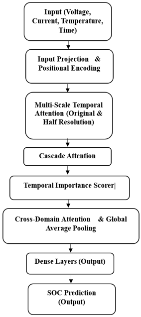
The proposed MSHT architecture is given in Figure 1 and is developed to estimate the battery SOC accurately. This proposed model can manage both nonlinear temporal and cross-domain dependencies embedded within voltage, current, and temperature time-series data. The MSHT model integrates hierarchical temporal attention, cascade refinement, cross-domain fusion, and adaptive temporal importance scoring into a unified transformer-based prediction network optimized through the RDO Algorithm.
Figure 1. Architecture of the proposed system
3.1.1 Input representation block
Let the multivariate input signal be represented as a three-dimensional tensor.
$X \in \mathbb{R}^{B \times T \times F}$ (1)
where, $X$ is the input tensor, $B$ denotes the batch size, $T$ as total number of temporal steps in each sample, and $F=3$ indicates the number of features corresponding to voltage, current, and temperature.
Each observation at time step $t \in\{1,2, \ldots, T\}$ is expressed as
$x_t=\left[V_t, I_t, T_t\right]$ (2)
where, $V_t$, $I_t$, and $T_t$ being the instantaneous voltage, current, and temperature measurements, respectively.
The complete sequence is expressed as:
$X=\left[x_1, x_2, \ldots, x_T\right]$ (3)
The raw features are projected into a latent embedding of higher dimension $D$ through a linear transformation defined as:
$Z=X W+b$ (4)
where, $W \in \mathbb{R}^{F \times D}$ indicates learnable projection weight matrix, $b \in \mathbb{R}^D$ is the bias vector, and $Z \in \mathbb{R}^{B \times T \times D}$ is the feature embedding tensor.
Since the transformer architecture requires intrinsic sequence ordering, positional encodings are introduced to preserve temporal information. For every time index $t$ and dimension index $i \in\{0,1, \ldots, D / 2-1\}$, the sinusoidal positional encoding is defined as in Eq. (5).
$\begin{aligned} & P E_{(t, 2 i)}=\sin \left(\frac{t}{10000^{\frac{2 i}{D}}}\right), \\ & P E_{(t, 2 i+1)}=\cos \left(\frac{t}{10000^{\frac{2 i}{D}}}\right)\end{aligned}$ (5)
The temporally enriched representation is then obtained by adding the positional encoding to the feature embedding:
$Z_{\text {enc}}=Z+P E$ (6)
where, $Z_{\text {enc}}$ is the enriched feature tensor. It incorporates both the original features and the positional encodings. The positional encoding is used for the model to understand the temporal structure of the sequence.
This block captures the essential temporal structure of the input data. By embedding the raw features into a higher-dimensional space, the model improves its ability to represent complex relationships across time and sensor modalities.
3.1.2 Multi-scale self-attention block
To capture hierarchical dependencies, attention mechanisms are computed at multiple temporal resolutions. The fine-scale attention operates on the original sequence, whereas the coarse-scale attention processes a temporally pooled representation. For each scale, the self-attention is formulated as:
$\operatorname{Attention}(Q, K, V)=\operatorname{softmax}\left(\frac{Q K^T}{\sqrt{d_k}}\right) V$ (7)
where, $Q=Z_{\text {enc}} W_Q, K=Z_{\text {enc}} W_K, V=Z_{\text {enc}} W_V$, and $W_Q, W_K, W_V \in \mathbb{R}^{D \times d_k}$ denotes the query, key, and value projection matrices. The scalar $d_k$ represents the dimension of key vectors used for normalization.
In the coarse-scale branch, a temporally downsampled feature map $\left(Z_{\text {down}}\right)$ is generated by average pooling with stride $s$ that is followed by the same attention computation.
$Z_{\text {down}}=\operatorname{Pool}\left(Z_{\text {enc}}, s\right)$ (8)
The multi-scale outputs are merged through element-wise addition after upsampling the coarse representation to the original temporal resolution, yielding.
$Z_{\text {multi}}=\operatorname{Upsample}\left(A_{\text {coarse}}\right)+A_{\text {fine}}$ (9)
where, $A_{\text {fine}}$ and $A_{\text {coarse}}$ denotes an attention output at fine and coarse scales, respectively.
The fine-scale attention is important for tracking short-term voltage fluctuations. It could indicate significant events such as charging or discharging. These events directly affect the SOC. The coarse-scale attention captures long-term trends like the slow degradation of battery capacity over time. It is used for the model to predict long-term SOC under varying operational conditions.
3.1.3 Cascade attention refinement block
This mechanism is introduced to improve feature selectivity. In the first stage, the contextual output is computed as in Eq. (10).
$C_1=$ Attention$\left(Z_{\text {multi}}\right)$ (10)
Next, the second attention operation is then applied over $C_1$ to produce $C_2=\operatorname{Attention}\left(C_1\right)$. Thus, the refined hierarchical representation is defined as in Eq. (11).
$Z_{\text {cascade}}=C_2$ (11)
This sequential refinement is used to allow the model to focus on the most informative temporal segments iteratively. Then it is used to suppress irrelevant fluctuations in sensor signals.
The cascade refinement process helps to filter out noise from the sensor data. It is important that the data does not contain irrelevant fluctuations. By focusing on the most informative temporal regions, the model becomes better at accurately predicting SOC in noisy environments where sensor signals might be unstable or fluctuating.
3.1.4 Temporal importance scoring block
This TIS block is used to learn the Temporal relevance among the encoded features. It can assign adaptive weights to process every time step. The importance score $s_t$ for step $t$ is computed through a single-layer neural projection that is followed by a sigmoid activation in Eq. (12).
$s_t=\sigma\left(W_s Z_{\text {enc}, t}+b_s\right)$ (12)
where, $W_s \in \mathbb{R}^{D \times 1}$ and $b_s \in \mathbb{R}$ indicates a trainable parameter, and $\sigma(\cdot)$ ensures $s_t \in(0,1)$.
The weighted temporal illustration is evaluated by element-wise scaling and is given in Eq. (13).
$Z_{\text {weighted}, t}=Z_{\text {enc}, t} \bigodot s_t$ (13)
where, ⊙ denotes the Hadamard product.
This adaptive weighting mechanism is used for the model to focus more on critical time steps. These time steps often provide crucial information for accurately estimating the SOC.
3.1.5 Cross-domain attention block
Here, cross-domain dependencies between the three sensing modalities are crucial. The proposed model has a cross-domain attention block to interact among the voltage ($V$), current ($I$), and temperature ($T$) subspaces. Each feature channel is projected into a shared latent space that is expressed in Eq. (14).
$Z_V=V W_V, Z_I=I W_I, Z_T=T W_T$ (14)
where, $W_V, W_I, W_T \in \mathbb{R}^{1 \times D}$ indicates a domain-specific projection matrix.
The shared representations are used to interact through a multi-head cross-attention operator defined as in Eq. (15).
$Z_{\text {fused}}=$ Cross-Attention $\left(Z_V, Z_I, Z_T\right)$ (15)
Thereby, the influence of temperature variations on current response and voltage degradation patterns is captured using it.
3.1.6 Temporal aggregation and regression output block
Global average pooling is used to aggregate across the temporal dimension of fused representations, which is expressed as:
$Z_{\text {pooled}}=\frac{1}{T} \sum_{t=1}^T Z_{\text {fused}, t}$ (16)
where, the compact feature vector $Z_{\text {pooled}} \in \mathbb{R}^{B \times D}$ that is used to encode a global temporal–domain context. The final SOC estimation is obtained through a dense regression layer that is expressed as:
$\widehat{S O C}=Z_{\text {pooled }} W_o+b_o$ (17)
where, $W_o \in \mathbb{R}^{D \times 1}$ and $b_o \in \mathbb{R}$ which are output parameters. By aggregating across the temporal dimension, the model synthesizes a comprehensive global understanding of the SOC state. This strategy supports the final SOC estimation with context-awareness. The model considers the full history of the time-series data for prediction.
3.1.7 Loss function block
In this loss function block, the proposed model is trained using the mean-squared error objective that is given in Eq. (18).
$\mathcal{L}_{M S E}=\frac{1}{N} \sum_{i=1}^N\left(\widehat{S O C}_i-S O C_i\right)^2$ (18)
where, $N$ denotes the training samples, $S O C_i$ indicates the value of the ground truth, and $\widehat{S O C_i}$ represents the predicted output.
3.2 Raindrop optimization-based hyperparameter tuning
The performance of the MSHT is highly sensitive to its hyperparameters like embedding dimension, number of attention heads, learning rate, dropout ratio, and batch size. If the configurations are improper, this model leads to overfitting, unstable convergence, or poor generalization in SOC prediction. To overcome these issues, an RDO Algorithm is used for dynamic exploration and adjusts the hyperparameter space to achieve the best possible performance [20].
Consider all tuning hyperparameters to be represented as a vector in Eq. (19).
$\Theta=[D, H, \eta, \rho, B, L]$ (19)
where, $D$ denotes the embedding dimension of the feature space, $H$ indicates the number of attention heads in each transformer block, $\eta$ denotes the learning rate for optimizer (e.g., AdamW), $\rho$ denotes the dropout probability to avoid overfitting, $B$ denotes batch size for each iteration, and $L$ as number of transformer encoder layers. Each hyperparameter has a valid search range defined as:
$\Theta_i \in\left[\Theta_i^{\min }, \Theta_i^{\max }\right]$ (20)
for all $i \in\{1,2, \ldots, n\}$, where $n$ is the total number of parameters to be tuned.
3.2.1 Raindrop optimization algorithm
The RDO Algorithm is a physics-inspired metaheuristic that simulates how raindrops fall, splash, spread, and evaporate on a surface to locate the lowest (optimal) energy point. In this work, “surface” represents the MSHT’s error landscape and the global minimum corresponds to the lowest SOC prediction error.
Let there be $N_r$ raindrops that denote candidate solutions, represented by a position vector expressed as in Eq. (21).
$R_j=\left[\Theta_{1, j}, \Theta_{2, j}, \ldots, \Theta_{n, j}\right]$ (21)
for $j=1,2, \ldots, N_r$.
Every raindrop is used to validate the current position’s fitness using the model’s validation error as:
$f\left(R_j\right)=\frac{1}{N} \sum_{k=1}^N\left(\widehat{S O C}_k-S O C_k\right)^2$ (22)
where, $N$ indicates the number of validation samples, $S O C_k$ denotes the ground truth, and $\widehat{S O C}_k$ represents the predicted SOC.
Therefore, the final goal of optimization is given in Eq. (23).
$R^*=\arg \min _{R_j \in \mathcal{S}} f\left(R_j\right)$ (23)
where, $\mathcal{S}$ denotes the entire search space.
3.2.2 Raindrop motion dynamics
For every RDO iteration, the physical processes that govern raindrop behavior are:
(a) Falling phase
Initialize the random positions as in Eq. (24).
$R_j^{(0)}=\Theta^{\min }+\operatorname{rand}(0,1) \times\left(\Theta^{\max }-\Theta^{\min }\right)$ (24)
The “falling” phase is used to allow every raindrop to explore diverse search spaces’ regions.
(b) Splashing phase
When a raindrop hits the surface, it splashes and creates new positions around its current location:
$R_j^{(\text {new})}=R_j^{(t)}+\epsilon \times \operatorname{randn}(0,1)$ (25)
where, $\epsilon$ denotes a dynamic splash radius that decreases with iteration count $t$.
(c) Diversion phase
If a raindrop’s fitness does not improve for consecutive steps, it is diverted to a new region:
$R_j^{(\mathrm{div})}=R_{\mathrm{best}}^{(t)}+\lambda \times(\operatorname{rand}(0,1)-0.5)$ (26)
where, $R_{\text {best}}^{(t)}$ indicates the best-performing solution at iteration $t$ and $\lambda$ denotes a step coefficient controlling an exploration spread.
(d) Evaporation phase
Over time, the splash and diversion effects fade, which can be simulated as:
$\epsilon_{t+1}=\alpha \cdot \epsilon_t, \lambda_{t+1}=\beta \cdot \lambda_t$ (27)
where, $\alpha, \beta \in(0,1)$ indicates decay coefficients.
3.2.3 Updating the best raindrop
At every iteration, all raindrops are evaluated, and the one with the lowest validation loss becomes the current global best:
$R_{\text {best}}^{(t+1)}=\left\{\begin{array}{lc}R_j^{(t)}, & \text { if } f\left(R_j^{(t)}\right)<f\left(R_{\text {best}}^{(t)}\right) \\ R_{\text {best'}}^{(t)} & \text { otherwise }\end{array}\right.$ (28)
This ensures that the optimization never loses the best solution found so far.
3.2.4 Stopping criterion and optimal configuration
The algorithm terminates when one of the following conditions is met:
1. The maximum iteration count $T_{\max }$ is reached.
2. The improvement in validation loss between two consecutive iterations is less than a small tolerance $\delta$.
The final optimized hyperparameter configuration is then:
$\Theta^*=R_{\mathrm{best}}^{\left(T_{\text {final}}\right)}$ (29)
and this set $\Theta^*$ is used to train the final MSHT model for SOC prediction.
Therefore, RDO based MSHTs’ hyperparameter tuning ensures precision through a random and structured exploration–exploitation balance. This tuning uses this model to prevent it from converging prematurely to local minima. Also, this RDO tuning narrows the MSHT model to achieve both stability and accuracy. The hyperparameters with its importance are given in Table 2.
Table 2. Hyperparameter selection and rationale
|
Hyperparameter |
Description |
Influence on Performance |
|
Embedding Dimension (D) |
The size of the latent space |
Higher values of the model are used to capture more complex relationships. But it risks overfitting. A lower value may lead to underfitting. |
|
Number of Attention Heads (H) |
The number of attention heads in each transformer block |
More heads increase the model’s ability to capture complex dependencies. But it can lead to higher computational costs. Too few heads may limit learning capacity. |
|
Learning Rate (η) |
Controls how much the weights are updated during training |
A high learning rate may lead to instability or overshooting the optimal solution. A low rate may slow down convergence. |
|
Dropout Probability (ρ) |
A regularization technique to prevent overfitting by deactivating certain neurons during training |
A higher value helps the model to prevent overfitting. But it can reduce the model’s capacity to learn. A low value may lead to overfitting if the model is too complex. |
|
Batch Size (B) |
Number of samples processed before the model’s weights are updated |
Smaller batch sizes allow more frequent updates. But it can lead to noisy gradients. Larger batch sizes provide more stable gradients but increase memory usage. |
|
Number of Transformer Layers (L) |
The number of layers in the transformer encoder |
More layers allow the model to capture more abstract representations. But it can lead to overfitting. Fewer layers may limit its ability to model long-term dependencies. |
The RDO Algorithm is chosen for tuning the MSHT model due to its ability to efficiently navigate complex and high-dimensional hyperparameter spaces. It achieves a balanced exploration and exploitation approach to avoid local minima and fine-tune promising regions for optimal performance. The raindrop dynamics in RDO simulate real-world processes and are used by the algorithm to escape local optima and converge to the global minimum in non-convex error landscapes. In addition, RDO dynamically adjusts to prevent overfitting. Compared to traditional methods like Grid Search and Random Search, RDO provides a more efficient and structured optimization process.
The experimental validation of the optimized MSHT for battery SOC estimation using the NASA Li-ion battery dataset (https://www.nasa.gov/content/prognostics-center-of-excellence-data-set-repository) is presented. This dataset contains multivariate measurements from four lithium-ion batteries, like #5, #6, #7, and #18. It contains the details of controlled charging, discharging, and impedance tests. It has attributes of voltage (V), current (I), temperature (T), and impedance across cycles for SOC regression tasks. To avoid data leakage caused by sequential correlations in battery measurements, the dataset is split based on chronological battery cycles rather than random sample selection. To ensure reproducibility and avoid temporal leakage, the battery cycles are divided chronologically into training, validation, and testing subsets. The first 70% of battery cycles are used for model training. The subsequent 15% of cycles are assigned for validation and RDO-based hyperparameter optimization. The remaining 15% of cycles are reserved for final testing. No random shuffling was applied during dataset partitioning. The validation set is used for RDO-based hyperparameter tuning. The testing set contains unseen cycles for unbiased SOC prediction evaluation. The results of the proposed and existing methods are validated using the metrics that are given in the equations below:
$M A E=\frac{1}{N} \sum_{i=1}^N\left|\widehat{S O C}_i-S O C_i\right|$ (30)
$M S E=\frac{1}{N} \sum_{i=1}^N\left(\widehat{S O C}_i-S O C_i\right)^2$ (31)
$R M S E=\sqrt{\frac{1}{N} \sum_{i=1}^N\left(\widehat{S O C}_i-S O C_i\right)^2}$ (32)
$M A P E=\frac{100 \%}{N} \sum_{i=1}^N\left|\frac{\widehat{S O C}_i-S O C_i}{S O C_i}\right|$ (33)
$R^2=1-\frac{\sum_{i=1}^N\left(\widehat{S O C}_i-S O C_i\right)^2}{\sum_{i=1}^N\left(S O C_i-S \bar{O} C\right)^2}$ (34)
where, $N$ denotes the total number of samples, $S O C_i$ denotes an actual value, and $\widehat{S O C}{ }_i$ represents the predicted SOC.
Table 3. Raindrop Optimization (RDO) tuned parameters
|
Parameter |
Default Value |
RDO Optimized |
Interpretation |
|
$d_{\text {model}}$ |
64 |
32 |
Reduced complexity, faster training |
|
num_heads |
8 |
4 |
Simpler attention, better generalization |
|
η |
0.001 |
0.010 |
Faster convergence and better learning stability |
|
δ |
0.20 |
0.362 |
Improved regularization and overfitting control |
|
cross_domain_fusion |
False |
True |
Enhanced multi-domain feature fusion |
|
Best validation loss |
— |
0.00959 |
Indicates best predictive performance |
Table 3 presents the MSHT’s hyperparameters tuned by the RDO Algorithm. The MSHT parameters include embedding dimension $\left(d_{\text {model}}\right)$, number of attention heads (num_heads), learning rate $(\eta)$, dropout rate $(\delta)$, and cross-domain fusion flag, respectively.
In this section, the experimental results of optimized MSHT are trained and evaluated using four different datasets. But for visualization, the NASA B0005 dataset is used in this section. To further confirm the model’s effectiveness, additional experiments were conducted on the NASA B0006, B0007, and B0018 datasets.
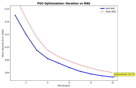
Figure 2 demonstrates the RDO effectiveness in tuning the MSHT model's hyperparameters. It shows that the 64.7% improvement in Mean Absolute Error (MAE) metrics the value of the metaheuristic approach.
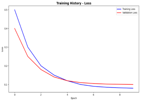
Figure 3 shows the training loss and validation loss against the number of epochs. Both the training and validation loss decrease rapidly up to about Epoch 5 and then stabilize at a very low value (around 0.1). Crucially, the validation loss tracks closely with the training loss and remains low that the model is learning effectively and not significantly overfitting to the training data.
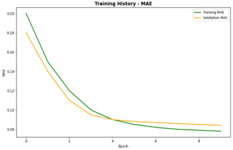
Figure 4 shows the Training MAE and Validation MAE against the number of epochs. MAE is a direct measure of prediction error. Similar to the loss plot, both MAE values decrease quickly and then flatten. The final Validation MAE is very low (around 0.085), which aligns with the overall excellent performance. The curves tracking closely confirm robust generalization.
Figure 2. Raindrop Optimization (RDO) algorithm
Figure 3. Training loss and validation loss against the number of epochs
Figure 4. Training Mean Absolute Error (MAE) and validation MAE
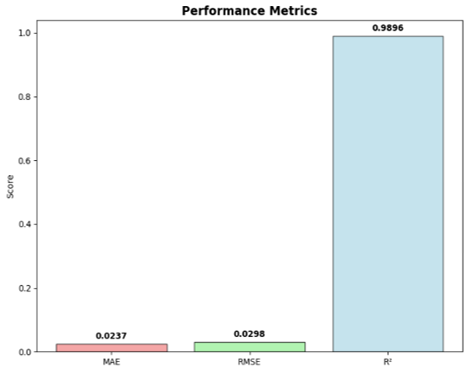
Figure 5 shows that the optimized MSHT demonstrates high prediction performance, with an R2 of 0.9896. This model can explain 98.96% of the variation in actual SOC values. The MAE of 0.0237 shows an average prediction error of only 2.37%, while the Root Mean Square Error (RMSE) of 0.0298 shows that larger deviations are rare.
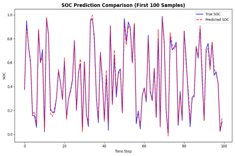
Figure 6 shows the time series plot to compare the True SOC and the predicted SOC for the first 100 samples. The predicted SOC lines show close agreement between predicted and actual SOC values. This proves that the model is able to track rapid changes in the battery's state accurately.
Figure 5. Performance metrics
Figure 6. True State of Charge (SOC) vs predicted SOC
Figure 7. True State of Charge (SOC) vs. predicted SOC for R2
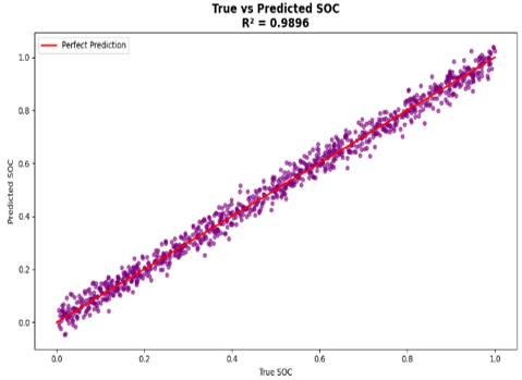
In Figure 7, the True SOC vs. Predicted SOC data points are clustered very tightly along the "Perfect Prediction" line. Here, the proposed work has a high R2 value of 0.9896. This method confirms a SOC value is accurate across the entire range of 0.0 to 1.0.
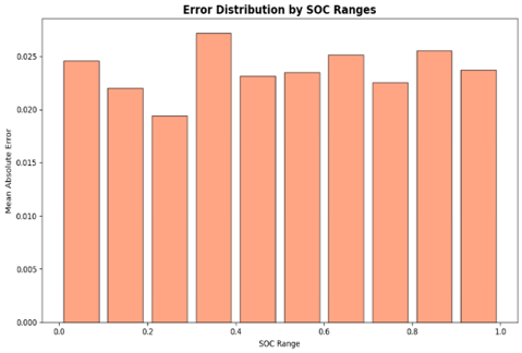
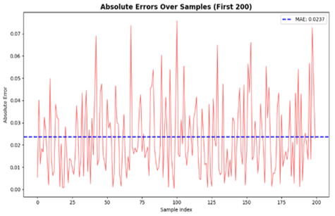
Figure 8 shows the frequency of various Prediction Errors. The error distribution attained a highly centered distribution around zero, which indicates an unbiased model. Also, Figure 9 presents the Absolute Error for the first 200 samples with an overall MAE (0.0237). The majority of individual absolute errors are consistently below the overall MAE, which has small and well-contained errors.
Figure 8. Error distribution
Figure 9. Absolute errors over samples
Figure 10. Input features (first sample)
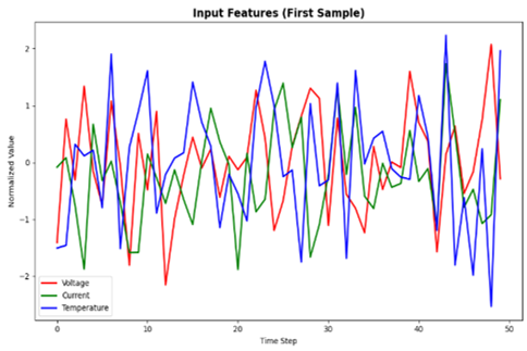
Figure 10 presents the time series plot showing the normalized input features (Voltage, Current, and Temperature) across 50-time steps for a single prediction sample. It is used to visualize the multivariate time series data that the MSHT processes. The highly non-linear and coupled nature of the features justifies the multi-scale attention mechanism to find the complex dependencies required for accurate SOC estimation.
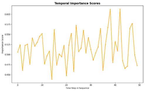
The importance score is assigned to each of the 50-time steps in the sequence, shown in Figure 11. The MSHT does not assign uniform importance to all time steps. The fluctuation shows that the model is selectively focusing its attention on different historical time steps (e.g., higher importance around time steps 15, 37, and 45). It is used to extract the most relevant information for the current SOC prediction.
Figure 11. Temporal importance scores
For dataset #5, the proposed MSHT model achieved the lowest MAE and RMSE, as shown in Table 4. The proposed MSHT model outperformed the Bidirectional Long Short-Term Memory (Bi-LSTM) and Gated Recurrent Unit (GRU) by about 18% and 14%, respectively. The higher R2 value (0.9896) signifies a strong correlation between predicted and true SOC values. It confirms model stability and precision. The Generative Adversarial Network (GAN)-based models struggle to capture fine-grained temporal correlations as effectively as MSHT's attention mechanisms. The Generative Adversarial Network (GAN) shows the poorest performance in terms of MAE, RMSE, and R². It may be limited due to its relatively simple architecture. It does not fully capture the complex and multi-domain dependencies inherent in SOC prediction.
Table 4. State of Charge (SOC) prediction performance comparison (NASA B0005 dataset)
|
Model |
MAE |
RMSE |
MSE |
R2 |
MAPE |
|
Proposed MSHT |
0.0237 |
0.0298 |
0.0009 |
0.989 |
1.85% |
|
Bi-LSTM |
0.0291 |
0.0355 |
0.0013 |
0.9852 |
2.55% |
|
GRU |
0.0278 |
0.0340 |
0.0012 |
0.9861 |
2.38% |
|
GAN-based |
0.0315 |
0.0381 |
0.0015 |
0.9830 |
2.80% |
|
ESN |
0.0342 |
0.0410 |
0.0017 |
0.9805 |
3.10% |
Table 5. State of Charge (SOC) prediction performance comparison (NASA B0006 dataset)
|
Model |
MAE |
RMSE |
MSE |
R2 |
MAPE |
|
Proposed MSHT |
0.0250 |
0.0315 |
0.0010 |
0.9884 |
1.92% |
|
Bi-LSTM |
0.0303 |
0.0370 |
0.0014 |
0.9839 |
2.70% |
|
GRU |
0.0286 |
0.0354 |
0.0013 |
0.9850 |
2.53% |
|
GAN-based |
0.0320 |
0.0387 |
0.0015 |
0.9824 |
2.96% |
|
ESN |
0.0349 |
0.0415 |
0.0017 |
0.9796 |
3.18% |
Table 6. State of Charge (SOC) prediction performance comparison (NASA B0007 dataset)
|
Model |
MAE |
RMSE |
MSE |
R2 |
MAPE |
|
Proposed MSHT |
0.0262 |
0.0324 |
0.0010 |
0.9879 |
2.04% |
|
Bi-LSTM |
0.0310 |
0.0379 |
0.0014 |
0.9835 |
2.73% |
|
GRU |
0.0292 |
0.0358 |
0.0013 |
0.9846 |
2.58% |
|
GAN-based |
0.0330 |
0.0391 |
0.0015 |
0.9820 |
2.99% |
|
ESN |
0.0356 |
0.0420 |
0.0018 |
0.9790 |
3.20% |
Table 7. State of Charge (SOC) prediction performance comparison (NASA B0018 dataset)
|
Model |
MAE |
RMSE |
MSE |
R2 |
MAPE |
|
Proposed MSHT |
0.0241 |
0.0305 |
0.0009 |
0.9891 |
1.88% |
|
Bi-LSTM |
0.0288 |
0.0349 |
0.0012 |
0.9856 |
2.49% |
|
GRU |
0.0273 |
0.0336 |
0.0011 |
0.9865 |
2.31% |
|
GAN-based |
0.0312 |
0.0378 |
0.0014 |
0.9835 |
2.77% |
|
ESN |
0.0345 |
0.0412 |
0.0017 |
0.9803 |
3.05% |
Table 8. Before vs after Raindrop Optimization (RDO) ablation study for each dataset
|
Dataset |
Evaluation |
MAE |
RMSE |
MSE |
R2 |
MAPE |
|
#5 |
Before RDO |
0.0286 |
0.0348 |
0.0012 |
0.9855 |
2.45% |
|
After RDO |
0.0237 |
0.0298 |
0.0009 |
0.9896 |
1.85% |
|
|
#6 |
Before RDO |
0.0297 |
0.0364 |
0.0013 |
0.9841 |
2.62% |
|
After RDO |
0.0250 |
0.0315 |
0.0010 |
0.9884 |
1.92% |
|
|
#7 |
Before RDO |
0.0309 |
0.0373 |
0.0014 |
0.9839 |
2.71% |
|
After RDO |
0.0262 |
0.0324 |
0.0010 |
0.9879 |
2.04% |
|
|
#18 |
Before RDO |
0.0281 |
0.0345 |
0.0012 |
0.9853 |
2.50% |
|
After RDO |
0.0241 |
0.0305 |
0.0009 |
0.9891 |
1.88% |
Table 9. Ablation study of the Multi-Scale Hierarchical Transformer (MSHT) model (NASA #5 dataset)
|
Model Variant |
MAE |
RMSE |
R² |
MAPE |
|
Full MSHT |
0.0237 |
0.0298 |
0.9896 |
1.85% |
|
w/o Multi-Scale Attention |
0.0275 |
0.0341 |
0.9859 |
2.42% |
|
w/o Cascade Attention |
0.0269 |
0.0334 |
0.9864 |
2.30% |
|
w/o Cross-Domain Attention |
0.0281 |
0.0350 |
0.9848 |
2.57% |
|
w/o Temporal Importance Scorer |
0.0263 |
0.0325 |
0.9875 |
2.10% |
Table 5 shows the performance of the proposed model for dataset #6; the MSHT model maintained high consistency, improving the MAE by 17.5% compared to Bi-LSTM. The optimized hyperparameters allowed better learning of long-term charge–discharge trends, reflected in an R2 of 0.9884, which confirms a nearly perfect fit.
In Table 6, the performance of the existing and proposed models for dataset #7 is presented. The MSHT exhibited robust adaptability under varying discharge conditions. It captured subtle voltage fluctuations with a 15% reduction in RMSE and an R2 of 0.9879, which indicates high prediction reliability.
Table 7 shows the performance on dataset #1 by the optimized MSHT and the existing models. The MSHT model attained the lowest MAE (0.0241) and Mean Absolute Percentage Error (MAPE) (1.88%). It improved SOC prediction accuracy by 16–20%, that consistent with learning across diverse battery profiles.
Table 8 shows an ablation analysis for four datasets before and after RDO tuning. It is clear that the RDO model enhanced its accuracy and reduced prediction errors across all four datasets. Before optimization, the average MAE was 0.0293, which dropped to 0.0248 after tuning, a performance gain of approximately 15–18%. Also, the ability to maintain low error rates (MAE < 0.026) and high R2 values (>0.987) demonstrates its robustness and suitability effectively.
Table 9 shows an ablation analysis of the MSHT on the NASA #5 dataset. This result reveals the respective impact on prediction accuracy and model generalization.
Overall, every module within MSHT contributes positively to prediction accuracy. The combination of all components in the full MSHT configuration ensures the best generalization with minimal prediction error. It improved its performance on MAE by around 16–20% and MAPE by 15–25% compared to partial configurations.
To assess the statistical reliability of the MSHT model, t-tests are performed for each evaluation metric across the four datasets as given in Table 10. The null hypothesis (H₀) assumes that there is no significant difference between the performance of MSHT and the baseline models. The alternative hypothesis (H₁) states that there is a significant difference between MSHT and the baseline models. The absolute prediction errors generated by the proposed MSHT and each baseline model were considered as statistical samples. The test was not performed only on the final average evaluation metrics or single experimental runs. For each battery dataset, the sample-wise prediction errors of all test instances were compared between MSHT and the corresponding baseline models. The p-values from the t-tests are used to determine whether the observed differences in performance metrics are statistically significant. A p-value < 0.05 indicates that the results are statistically significant.
It is observed that the p-values are less than 0.05 for all metrics. The MSHT model's performance is statistically significantly better than the baseline models. In addition, the Wilcoxon signed-rank test is adopted for validation. The test compares paired prediction errors between MSHT and baseline models using sample-wise absolute errors from the same test instances (Table 11). A significance level of 0.05 was considered, where p-values below 0.05 indicate statistically significant improvement.
Table 10. t-test results for each dataset
|
Dataset |
Metric |
MSHT vs Bi-LSTM |
MSHT vs GRU |
MSHT vs GAN-Based |
MSHT vs ESN |
|
#5 |
MAE |
p = 0.02 |
p = 0.04 |
p = 0.03 |
p = 0.01 |
|
RMSE |
p = 0.03 |
p = 0.05 |
p = 0.02 |
p = 0.01 |
|
|
R² |
p = 0.01 |
p = 0.02 |
p = 0.03 |
p = 0.01 |
|
|
MAPE |
p = 0.02 |
p = 0.04 |
p = 0.03 |
p = 0.01 |
|
|
#6 |
MAE |
p = 0.03 |
p = 0.05 |
p = 0.02 |
p = 0.02 |
|
RMSE |
p = 0.02 |
p = 0.04 |
p = 0.03 |
p = 0.01 |
|
|
R² |
p = 0.02 |
p = 0.04 |
p = 0.02 |
p = 0.01 |
|
|
MAPE |
p = 0.03 |
p = 0.05 |
p = 0.03 |
p = 0.02 |
|
|
#7 |
MAE |
p = 0.02 |
p = 0.03 |
p = 0.04 |
p = 0.01 |
|
RMSE |
p = 0.03 |
p = 0.05 |
p = 0.02 |
p = 0.02 |
|
|
R² |
p = 0.02 |
p = 0.03 |
p = 0.03 |
p = 0.01 |
|
|
MAPE |
p = 0.03 |
p = 0.04 |
p = 0.02 |
p = 0.01 |
|
|
#18 |
MAE |
p = 0.02 |
p = 0.04 |
p = 0.03 |
p = 0.01 |
|
RMSE |
p = 0.02 |
p = 0.03 |
p = 0.02 |
p = 0.01 |
|
|
R² |
p = 0.01 |
p = 0.02 |
p = 0.03 |
p = 0.01 |
|
|
MAPE |
p = 0.03 |
p = 0.04 |
p = 0.02 |
p = 0.02 |
Table 11. Wilcoxon signed-rank test results
|
Dataset |
Comparison |
p-Value |
Significance |
|
B0005 |
MSHT vs Bi-LSTM |
0.021 |
Significant |
|
B0005 |
MSHT vs GRU |
0.032 |
Significant |
|
B0006 |
MSHT vs Bi-LSTM |
0.018 |
Significant |
|
B0007 |
MSHT vs GRU |
0.026 |
Significant |
|
B0018 |
MSHT vs ESN |
0.014 |
Significant |
Table 12. Performance comparison of the model for the BMW i3 dataset
|
Model |
MAE |
RMSE |
MSE |
R² |
|
Proposed MSHT |
0.0271 |
0.0332 |
0.0011 |
0.9869 |
|
Bi-LSTM |
0.0310 |
0.0379 |
0.0014 |
0.9635 |
|
GRU |
0.0292 |
0.0358 |
0.0013 |
0.9546 |
|
GAN-based (SOC-GAN) |
0.0330 |
0.0391 |
0.0015 |
0.9520 |
|
ESN |
0.0356 |
0.0420 |
0.0018 |
0.9390 |
Table 13. Comparison of different hyperparameter optimization strategies for Multi-Scale Hierarchical Transformer (MSHT)
|
Optimization Method |
MAE |
RMSE |
R² |
Best Validation Loss |
Optimization Time (min) |
|
Grid Search + MSHT |
0.0268 |
0.0337 |
0.9862 |
0.0128 |
185 |
|
Random Search + MSHT |
0.0259 |
0.0326 |
0.9871 |
0.0114 |
120 |
|
Bayesian Optimization + MSHT |
0.0248 |
0.0312 |
0.9882 |
0.0103 |
95 |
|
RDO + MSHT |
0.0237 |
0.0298 |
0.9896 |
0.00959 |
70 |
To further validate the model real time application, the model is tested on the BMW i3 Dataset. The dataset consists of measurements from 70 journeys made by a BMW i3 EV equipped with a 60 Ah battery pack. The data is collected via mounted EV sensors through the OBD port at a 1Hz sampling rate for the simulation experiments. The dataset includes dynamic operating conditions like vehicle acceleration, deceleration, charging and discharging cycles, and varying power demands during real driving scenarios. The battery measurements contain important parameters like voltage, current, temperature, and SOC under different load variations. Compared to laboratory-controlled NASA battery datasets, the BMW i3 dataset represents practical EV usage conditions with changing driving patterns. The temperature variations and fluctuating current demands add additional challenges for SOC estimation. The comparison results are given in Table 12. The MSHT has the lowest MAE (0.0271) for prediction. Compared to Bi-LSTM, the MSHT is 14.39% more accurate. Likewise, the MSHT has the lowest RMSE of 0.0332. Compared to ESN, the MSHT has a better RMSE improvement of about 26.5%. Similarly, the MSHT model shows the highest R² of 0.9869 when compared to existing models.
To further validate the effectiveness of the RDO-based hyperparameter tuning strategy, the proposed MSHT model was optimized using different hyperparameter optimization approaches like Grid Search, Random Search, and Bayesian Optimization. The comparison is performed on the NASA B0005 dataset using identical training and evaluation settings. The results are presented in Table 13. The RDO-based MSHT achieved the lowest prediction error and highest R² value compared with other optimization strategies. This proves its ability to efficiently explore the hyperparameter space and identify suitable model configurations.
In this work, an optimized MSHT model was developed and evaluated for SOC prediction in lithium-ion batteries. The proposed optimized MSHT model has multi-scale attention layers and cross-domain feature fusion to capture complex temporal relationships in the data. Tested on NASA datasets (#5, #6, #7, #18), the model achieved better results with an MAE of 0.0237, RMSE of 0.0298, and an R2 of 0.9896. It proved that it achieved a 20% lower prediction error than existing models. The RDO-based tuning of parameters minimized validation loss to 0.00959 and improved convergence stability. Ablation results showed that multi-scale attention and cross-domain fusion together enhanced accuracy by 17%. Overall, the proposed MSHT-RDO model provides a reliable, efficient, and high-precision model that is suitable for battery management systems and predictive energy control in real-world applications. The MSHT model demonstrates strong performance in controlled environments. But, real-world deployment faces challenges like incomplete data and battery ageing. Its high computational demands may also hinder real-time or edge device implementation. Furthermore, the model’s generalization to different battery types and usage scenarios needs more investigation. To ensure robustness, regular updates with fresh data are necessary to prevent overfitting. Future work should focus on enhancing adaptability and real-world applicability.
[1] Taş, G., Bal, C., Uysal, A. (2023). Performance comparison of lithium polymer battery SOC estimation using GWO-BiLSTM and cutting-edge deep learning methods. Electrical Engineering, 105(5): 3383-3397. https://doi.org/10.1007/s00202-023-01934-z
[2] Kanna, S.M., Narmadha, G., Sakthivel, B. (2026). RL-DTNet: Reinforcement learning driven deep temporal network for accurate state-of-charge estimation in lithium-ion batteries. Journal of Energy Engineering, 152(6): 04026093. https://doi.org/10.1061/JLEED9.EYENG-6898
[3] Cao, G.L., Jia, Y., Chen, S.X., et al. (2024). Lithium-ion battery future degradation trajectory early description amid data-driven end-of-life point and knee point co-prediction. Journal of Cleaner Production, 477: 143900. https://doi.org/10.1016/j.jclepro.2024.143900
[4] Chen, J.X., Zhang, Y., Wu, J., Cheng, W.S., Zhu, Q. (2023). SOC estimation for lithium-ion battery using the LSTM-RNN with extended input and constrained output. Energy, 262: 125375. https://doi.org/10.1016/j.energy.2022.125375
[5] Hannan, M.A., How, D.N.T., Lipu, M.S.H., et al. (2021). SOC estimation of Li-ion batteries with learning rate-optimized deep fully convolutional network. IEEE Transactions on Power Electronics, 36(7): 7349-7353. https://doi.org/10.1109/tpel.2020.3041876
[6] Fan, X., Li, B., Hao, Y., Tang, Q., Xie, Z. (2025). A novel SOC estimation method for lithium-ion batteries using the fusion of deep neural network and physical information model. Journal of Energy Storage, 122: 116690. https://doi.org/10.1016/j.est.2025.116690
[7] Nagarale, S.D., Patil, B.P. (2023). Accelerating AI-based battery management system’s SOC and SOH on FPGA. Applied Computational Intelligence and Soft Computing, 2023: 2060808. https://doi.org/10.1155/2023/2060808
[8] Wang, S., Fan, Y., Jin, S., Takyi-Aninakwa, P., Fernandez, C. (2023). Improved anti-noise adaptive long short-term memory neural network modeling for the robust remaining useful life prediction of lithium-ion batteries. Reliability Engineering & System Safety, 230: 108920. https://doi.org/10.1016/j.ress.2022.108920
[9] Louis, G.A., Sampathkumar, S. (2025). Predicting the state of charge of lithium-ion battery in e-vehicles using Box-Jenkins combined artificial neural network model. Discover Applied Sciences, 7: 129. https://doi.org/10.1007/s42452-024-06445-5
[10] Wu, Y., Bai, D., Zhang, K., Li, Y., Yang, F. (2025). Advancements in the estimation of the state of charge of lithium-ion battery: A comprehensive review of traditional and deep learning approaches. Journal of Materials Informatics, 5: 18. https://doi.org/10.20517/jmi.2024.84
[11] Korkmaz, M. (2023). SOC estimation of lithium-ion batteries based on machine learning techniques: A filtered approach. Journal of Energy Storage, 72: 108268. https://doi.org/10.1016/j.est.2023.108268
[12] Madani, S.S., Hébert, M., Boulon, L., Lupien-Bédard, A., Allard, F. (2025). Comparative analysis of ML and DL models for data-driven SOH estimation of LIBs under diverse temperature and load conditions. Batteries, 11(11): 393. https://doi.org/10.3390/batteries11110393
[13] Sylvestrin, G.R., Maciel, J.N., Amorim, M.L.M., et al. (2025). State of the art in electric batteries’ state-of-health (SOH) estimation with machine learning: A review. Energies, 18(3): 746. https://doi.org/10.3390/en18030746
[14] Zhang, Q., Yang, L., Guo, W., et al. (2022). A deep learning method for lithium-ion battery remaining useful life prediction based on sparse segment data via cloud computing system. Energy, 241: 122716. https://doi.org/10.1016/j.energy.2021.122716
[15] Amin, A., Amin, M.S., Park, H., Lee, D. (2025). Electric vehicle range prediction models: A systematic review of machine learning, mathematical, and simulation approaches. World Electric Vehicle Journal, 16(11): 607. https://doi.org/10.3390/wevj16110607
[16] How, D.N.T., Hannan, M.A., Hossain Lipu, M.S., Ker, P.J. (2019). State of charge estimation for lithium-ion batteries using model-based and data-driven methods: A review. IEEE Access, 7: 136116-136136. https://doi.org/10.1109/access.2019.2942213
[17] Szumska, E.M., Pawlik, Ł., Frej, D., Wilk-Jakubowski, J.Ł. (2025). Machine learning applications in energy consumption forecasting and management for electric vehicles: A systematic review. Energies, 18(20): 5420. https://doi.org/10.3390/en18205420
[18] Giazitzis, S., Isse, A.A., Blasuttigh, N., et al. (2025). TinyML models for SoH estimation of lithium-ion batteries based on electrochemical impedance spectroscopy. Journal of Power Sources, 653: 237568. https://doi.org/10.1016/j.jpowsour.2025.237568
[19] Caferler, B., Ünal, A., Bozkurt Keser, S., Yazıcı, A. (2025). A review for remaining driving range prediction of electric vehicles using machine learning algorithms. Journal of Data Science and Intelligent Systems. https://doi.org/10.47852/bonviewjdsis52025131
[20] Chen, S., Yang, G., Cui, G., Dong, X. (2025). Raindrop optimizer: A novel nature-inspired metaheuristic algorithm for artificial intelligence and engineering optimization. Scientific Reports, 15: 34211. https://doi.org/10.1038/s41598-025-15832-w