Tarun Kumar* | Divya Lohani | Debopam Acharya
© 2026 The authors. This article is published by IIETA and is licensed under the CC BY 4.0 license (http://creativecommons.org/licenses/by/4.0/).
OPEN ACCESS
Accurate and scalable road surface condition monitoring is essential for intelligent transportation systems, yet practical smartphone-based solutions remain challenging due to sensor variability and severe class imbalance in real-world road datasets. This study proposes an imbalance-aware ensemble learning framework for multiclass road surface classification using smartphone inertial sensing. The proposed framework integrates six-channel accelerometer and gyroscope measurements with orientation-robust feature fusion, leakage-free data partitioning, imbalance mitigation, and heterogeneous classifier integration. Temporal and spectral features are extracted from inertial signals, while Synthetic Minority Over-sampling Technique with Edited Nearest Neighbors (SMOTEENN) is applied exclusively to the training data to improve minority-class representation. Four representative machine learning (ML) models, including AdaBoost, Support Vector Machine (SVM), Random Forest (RF), and a stacking ensemble, are systematically evaluated. Experimental results demonstrate that the stacking model achieves the best performance, obtaining an accuracy of 0.9883, macro-F1-score of 0.8843, and weighted-F1-score of 0.9880. The proposed approach improves recognition capability for minority road conditions while maintaining high overall classification reliability. Furthermore, a smartphone-based sensing application is developed to support practical data acquisition and real-time road-condition monitoring. The findings demonstrate the feasibility of combining inertial sensor fusion and imbalance-aware ensemble learning for cost-effective and scalable road surface assessment.
road surface classification, smartphone sensing, inertial sensor fusion, ensemble learning, class imbalance, machine learning
Road transportation infrastructures are regularly subjected to wear and tear resulting from weather conditions, traffic, and lack of maintenance. Road surface characteristics, such as potholes, rumble strips, and speed bumps, affect driving pleasure, vehicle condition, safety incidents, and traffic flow [1]. Although manual inspection procedures are costly and occasional, dedicated surveying vehicles are not always feasible for economic, large-scale, or periodic use. Currently available technologies for road pavement classification include 3D laser scanners and vision-based systems; however, these techniques suffer from high cost and vulnerability to environmental conditions [1]. This limits the scalability of their deployment. These limitations have led to the increasing popularity of smartphone-based sensing systems, where embedded inertial measurement unit (IMU) sensors can capture vibration signals related to road anomalies. Recent studies have demonstrated that combining smartphone sensors with machine learning (ML) can provide cost-effective alternatives to traditional survey vehicles [2, 3]. Advanced mobile-optimized learning platforms [4] have been developed as solutions for real-time road condition assessment, demonstrating classification accuracies exceeding 95% using smartphone IMU sensors [5].
Smartphones provide a convincing platform as they are low-cost, widely available, GPS-capable, and easy to integrate with cloud or edge analytics. However, real-world road anomaly classification from smartphone signals remains difficult because real-world datasets are usually imbalanced, anomaly events are short relative to smooth-road segments, and signals vary with speed, mounting conditions, and device orientation. In multiclass classification, a high overall accuracy can hide poor minority-class performance, making it essential to integrate imbalance-aware techniques [6].
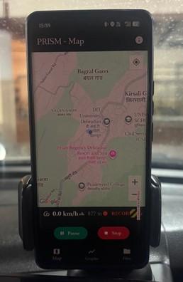
Another research issue is whether a leakage-free [7, 8], imbalance-aware classical ML pipeline can achieve high global accuracy while significantly enhancing performance on minority road-condition classes. Our work, which focuses on using smartphone sensing to collect and track road-condition data in Dehradun, Uttarakhand, India, contributes to both a research-oriented classification pipeline and an application-centric perspective. We utilized the smartphone-based IMU sensor for data acquisition through the Pavement Recognition and Intelligent Surface Monitoring (PRISM) application, which also facilitates road-event interaction and future live prediction. As shown in Figure 1, in our projected smartphone sensing system architecture, the smartphone was mounted on the dashboard of a four-wheeler using a holder, collecting motion data along the X, Y, and Z axes, which is sent to a server for processing and subsequent analytics.
The main contributions of this work are as follows:
(1) A complete smartphone inertial sensing pipeline using accelerometer and gyroscope streams collected through the PRISM application.
(2) Leakage-free training design in which data splitting is performed before imbalance handling.
(3) Sliding-window segmentation with class-purity filtering for event-focused sample construction.
(4) Rich time-domain and frequency-domain feature extraction from six inertial channels plus signal magnitudes.
(5) Augmentation of data to handle imbalance using Synthetic Minority Over-sampling Technique with Edited Nearest Neighbors (SMOTEENN) [9].
(6) Comparative evaluation of AdaBoost [10], Support Vector Machine-Radial Basis Function (SVM-RBF) [11], Random Forest (RF) [12], and Stacking [13].
Compared to the earlier studies outlined in Table 1, the current pipeline is characterized by four interrelated components instead of treating them separately: the integration of a six-channel accelerometer and gyroscope fusion as opposed to relying solely on single-sensor accelerometer data, a strictly leakage-free approach where the training/testing division occurs before any resampling, class-purity-filtered sliding windows that minimize label confusion at event boundaries, and a direct comparison among four different families of classifiers (boosting, kernel-based, bagging, and stacking) within a consistent SMOTEENN-balanced feature space. This combination enables the observed improvements to be attributed to the overall design of the pipeline rather than to an individual modeling decision.
Figure 1. The projected smartphone sensing system architecture
Classification of road surfaces has been widely researched owing to the potential applications for safety, optimal design of transportation infrastructure, and development of intelligent transportation systems. There are several studies that have successfully utilized smartphone sensors and ML algorithms in classifying road surfaces. This literature review summarizes the main approaches, data used, results, and limitations of recent papers dedicated to this topic.
Horizontal positioning of the accelerometer and gyroscope sensors found in smartphones proved highly efficient in the task of classifying road surfaces [14]. The authors of this paper recorded their data at a frequency of 100 Hz, gathering timestamps, three axes of acceleration, gyroscope readings, car speed, and GPS coordinates. These measures allowed attaining a 94% accuracy rate when determining the levels of road roughness. Ecological variables such as light or weather were sources of noise that interfered with the successful implementation of the algorithm. Accelerometer and gyroscope integration into ATVs allows pothole detection and International Roughness Index calculation [14] with an accuracy rate of 90.5% and an error rate of 8.41%, showcasing the utility of sensor-based methods across diverse vehicular conditions. Road condition evaluation using accelerometers and gyroscopes with the International Roughness Index metric was explored by Douangphachanh and Oneyama [15]. The use of AndroSensor in smartphones in different cars in areas around the gearshift led to R² coefficients ranging from 0.721 to 0.869. However, locating devices near the gearshift led to increased levels of engine noise, which may lead to inaccurate data; conversely, the dashboard was a better position to get more vibration data related to the road.
In the study by Ghafoor [16], pothole detection based on data from accelerometers and ultrasonic sensors resulted in impressive performance using Extreme Gradient Boosting (XGBoost); the model achieved an accuracy of 94.56%, recall of 97.41%, precision of 96.40%, and F1-score of 96.90%. In Bengaluru, India, Nericell [17] detected various forms of road surface damage using information from accelerometers in three types of vehicles. Although the number of false negatives decreased to 29% when well-oriented sensors were used, positioning variations continued to pose problems since the false negatives were high above 25 km/h. In the study by Afenika et al. [18], the classification of road surfaces into smooth and damaged conditions based on accelerometer data showed promising results. The authors’ dataset included 300 data sets, 200 sets for smooth roads and 100 for the damaged ones, and was analyzed through the SVM approach, resulting in 93% accuracy and demonstrating the high efficiency of the approach in road condition differentiation.
Classification of the road surface irregularities, such as potholes and bumps, was performed using the K-Nearest Neighbors (KNN) approach in combination with accelerometer sensors, which resulted in 96.03% pothole accuracy and 94.12% bump accuracy [19]. A related research study collected accelerometer and GPS data from an Android application, with a sampling frequency of 10 Hz on the roads of Chandigarh, India. Detection of potholes and bumps based on a Dynamic Time Warping (DTW) approach led to 88.66% accuracy for potholes and 88.89% for bumps; however, high computational costs prevented the authors from scaling up the test set [20]. The same DTW algorithm was implemented by other researchers to detect road markings, cracks, and potholes with the use of a smartphone gyroscope and frequency at 30 Hz [21].
The work [11] detected road conditions in Malaysia using an Android app, including acceleration signals from the 3-axis accelerometer. Their models achieved over 99% accuracy in classifying various road types, highlighting the potential of accelerometer-based classification. The study [22] examined how crowdsourced data from accelerometers and gyroscopes can be used for monitoring the condition of cycleways through GyroTracker software. They classified road segments into true bad, true okay, and true good, achieving a classification rate of about 90%. Another study investigated the use of deep learning algorithms for road surface detection and classification, such as detecting potholes and speed bumps [23]. Reservoir computing, Convolutional Neural Network (CNN), and Long Short-Term Memory (LSTM) achieved excellent results with accuracies up to 98%. However, the real-time implementation faced challenges related to computational requirements and processing speed. A crowdsensing-driven platform that utilizes smartphone GPS and accelerometer data was presented in Texas, USA, by the study [24] for detecting potholes and bumps. The system recorded geo-referenced Z-axis accelerations to evaluate road quality in poor, bad, and good categories. Basavaraju et al. [25] employed multi-class supervised learning approaches to classify road structures using smartphone data. Methods such as SVM, Decision Tree (DT), and Multilayer Perceptron (MLP) models were used to classify smooth roads, cracks, and potholes, with MLP achieving the highest average test accuracy of 91.49%. Limited training data was a key factor affecting accuracy. In another study, researchers focused on analyzing vehicle vibrations to detect humps and potholes, where prediction errors increased with increasing speeds up to 34.8% at 15 km/h and declined to 1.6% at 20 km/h. This study considered only accelerometer data but ignored the extra information that could be obtained from gyroscopes [26].
The study [27] suggested the utilization of accelerometer data and video statistics to detect road surface irregularities. Several approaches, such as thresholding, SVM, RF, LSTM, and joint optimization, have been investigated. Under the condition where the smartphone is fixed within the holder, LSTM and joint optimization resulted in accuracies of 0.82 and 0.92, respectively. For the case where the smartphone was placed within the car door compartment, LSTM and joint optimization yielded accuracies of 0.87 and 0.88, respectively. Table 1 summarizes the methodologies, dataset sizes, accuracies, key features, and limitations of recent studies in road surface classification, highlighting the strengths and gaps the proposed approach addresses.
Research on road anomaly monitoring has evolved from simple accelerometer peak detection and GPS-correlated thresholds to supervised ML and deep learning approaches, though early methods struggled with multiclass discrimination under varying conditions [1]. Subsequent supervised learning studies have improved multiclass separability using engineered temporal, statistical, and spectral features with models such as SVMs, RFs, and boosting algorithms, but class imbalance, where smooth-road samples vastly outnumber potholes and speed bumps, remains a persistent challenge that biases models toward majority classes despite high reported accuracy. Across these previous studies, several recurring limitations can be identified: dependence on a single inertial sensor instead of integrating data from multiple sensors, assessment conducted on insufficiently large datasets to reveal behaviors of minority classes, lack of strategies for managing imbalances with consideration for leakage, and minimal exploration of how the developed model would be implemented on the device as opposed to being evaluated in an offline context. This study also builds on our own progressive line of work on smartphone-based road surface classification. Earlier studies established a baseline for road surface classification using smartphone accelerometer and gyroscope data. Class imbalance was subsequently addressed through Synthetic Minority Over-sampling Technique (SMOTE)-augmented KNN classification, followed by an Adaptive Synthetic Sampling (ADASYN)-driven XGBoost framework for pothole detection [6].
Table 1. Comparison of prior road surface classification studies
|
Study |
Methodology |
Accuracy |
Key Feature(s) |
Limitations |
|
[11] |
Accelerometer, gyroscope, ML |
>99% |
Differentiates multiple road surface types |
Did not address class imbalance |
|
[14] |
Accelerometer, gyroscope |
94% |
3-axis acceleration and gyroscope data |
Sensitive to environmental noise |
|
[15] |
Accelerometer, gyroscope |
R² = 0.72–0.87 |
Uses the IRI metric for road roughness |
Impacted by engine noise due to smartphone placement near the gearshift |
|
[16] |
Accelerometer, XGBoost |
94.56% |
Combines accelerometer and ultrasonic sensors |
Focused only on pothole detection |
|
[17] |
Accelerometer, GPS, Nericell system |
False negative: 29% |
Monitors potholes and bumps |
Sensitive to speed and sensor orientation |
|
[18] |
Accelerometer, SVM |
93% |
Classifies smooth and damaged roads |
Limited to binary classification |
|
[19] |
Accelerometer, KNN |
96.03% (potholes) |
Multi-class road surface classification |
Limited to small-scale experiments |
|
[20] |
GPS, accelerometer, DTW |
88.66% (potholes) |
DTW on 6 smartphones |
Computationally expensive |
|
[23] |
CNN, LSTM, reservoir computing |
98% |
Pothole and bump detection using DL |
High computational requirements for real-time usage |
|
[25] |
Accelerometer, gyroscopes, and GPS |
91.49% |
SVM, DT, and MLP for classification |
A small dataset limits model generalizability |
|
[27] |
Accelerometer, video fusion, ML |
92% |
LSTM and joint optimization for anomalies |
Limited accuracy in smartphone holder setups |
Note: SVM = Support Vector Machine, XGBoost = Extreme Gradient Boosting, CNN = Convolutional Neural Network, LSTM = Long Short-Term Memory, ML = machine learning, DT = Decision Tree, MLP = Multilayer Perceptron, DTW = Dynamic Time Warping, KNN = K-Nearest Neighbors.
This study addresses these gaps through a comprehensive pipeline featuring six-channel inertial sensing (accelerometer + gyroscope feature-level fusion), leakage-free post-split SMOTEENN resampling, and comparative evaluation of heterogeneous ensembles (AdaBoost, SVM-RBF, RF, Stacking), while emphasizing practical mobile app deployment for real-world sensing, annotation, and inference, bridging the critical gap between offline accuracy and end-user deployment scenarios, and complementing the dual-filter deployment-focused study [28] with a broader comparative evaluation of classical imbalance-aware ensemble methods. This work also complies with the United Nations Sustainable Development Goals 9 and 11 [6, 29].
The proposed framework serves as a smartphone-centered road-surface sensing and analytics system. The hardware setup of our experiment is depicted in Figure 2, comprising a car, a smartphone, and a phone holder. The phone holder has been mounted on the car's dashboard near the front wheels to optimize accelerometer performance. Any contact between the road and the vehicle has the most significant impact near the wheels.
Figure 2. Hardware setup
The smartphone collects tri-axial accelerometer and tri-axial gyroscope data while the vehicle is in motion. These classifications are done by our models according to four types of road conditions: smooth road, speed bump, rumble strip, and pothole. The classification is performed through a combination of data obtained from accelerometers and gyroscopes, along with geographical coordinates of the road conditions. There are various processes involved in the workflow of the system as a whole: data acquisition, data segmentation, feature extraction, dealing with class imbalances, model training, and prediction generation. As for the components of the pipeline, the PRISM application on the Android platform is used as the front-end sensing interface, whereas the experimental notebook constitutes the backend for model development. This arrangement allows both offline and online model operation.
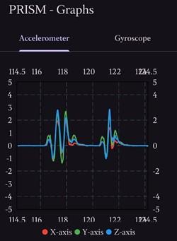
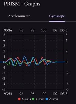
As presented in Figure 3, accelerometer channels primarily capture translational vibration and impact intensity, while gyroscope channels capture rotational motion and directional disturbance. Their joint use creates a richer representation of road-surface events than either modality alone. Table 2 presents the primary modules of the PRISM application.
(a)
(b)
Figure 3. PRISM application screenshots illustrating (a) accelerometer and (b) gyroscope signals
Table 2. Functional modules of the PRISM application
|
Module |
Description |
Sensors/Inputs |
Outputs |
|
Map Screen |
Real-time GPS tracking with IMU overlay and road event prediction |
GPS, Accelerometer, Gyroscope |
CSV recordings with timestamp, predictions, and orientation |
|
Graph Screen |
Live gravity-compensated accelerometer and gyroscope graphs |
Accelerometer, Gyroscope |
Real-time orientation (pitch/roll), sensor validation |
|
File Manager Screen |
CSV export, preview, sharing, Google Drive upload |
File system |
Shareable CSV files for ML pipeline |
|
IMU Sampler |
50Hz IMU sampling with gravity compensation |
AccX/Y/Z, GyroX/Y/Z (gravity-removed) |
6-channel time-series data |
|
Road Predictor |
Multi-sensor fusion prediction (simulation mode) |
Gravity-compensated Acc + Gyro magnitudes |
Class predictions (0 = Smooth, 1 = Speed Bump, 2 = Rumble Strip, 3 = Pothole) |
Note: IMU = inertial measurement unit, PRISM = Pavement Recognition and Intelligent Surface Monitoring.
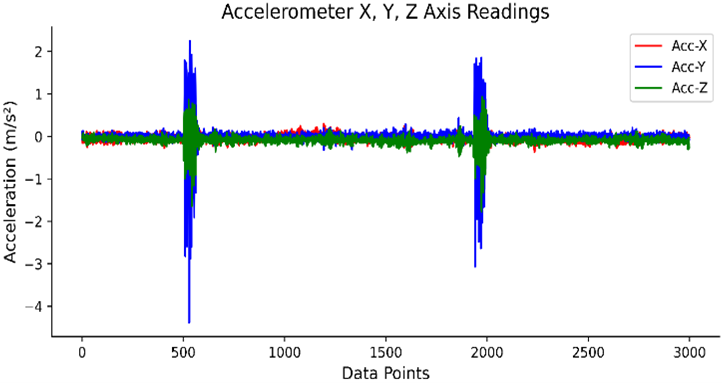
The accelerometers measure the rate at which a moving vehicle accelerates or decelerates in all three axes, giving us insights into peculiarities of the road surface. With a study of the frequency and intensity of vibrations, even minute variations such as bumps and other imperceptible characteristics can be observed. For instance, Figure 4(a) shows that when a vehicle is moving on a normal road, its values in the three axes remain stable. Once the car goes over a speed bump, the data produces a distinctive peak due to the rise of the car over the bump, then another peak indicates the compression of the suspension and the descent. After that, another peak illustrates the recoil of the suspension and the recovery of the car once it passes the speed bump. Conversely, Figure 4(b) represents the readings collected while the car passes through rumble strips. In contrast to speed bumps, rumble strips indicate a pattern of recurring crests and troughs on the sensor readings, where each crest or trough is related to the deflection of each rumble strip.
(a)
(b)
Figure 4. Illustration of accelerometer graphs depicting (a) speed bumps and (b) rumble strips
The recurrent waveform observed corresponds with the recurring nature of the arrangement of the rumble strips that are generally installed in close proximity to each other. The experiments covered a 500-meter section while maintaining an average speed of 30 kmph. The experimental site was selected to gather data encompassing all four class labels. The experiment was replicated over 100 instances on Rajpur Road, Dehradun, Uttarakhand (India), leading to a sizable dataset.
Ground-truth labels were assigned to each recording session during post-processing through a combination of observations made by on-road annotators, GPS-correlated event records, and visual analysis of the accelerometer waveforms. Events were identified using GPS waypoints on the route map for each session. The front-seated annotator pressed a button in the PRISM app at both the beginning and end of every event. Synchronization of GPS timestamps was maintained within approximately ±0.5 seconds around each marked event. Additionally, as part of quality control, all windows drawn from minority classes were re-evaluated post hoc for a visible impulse response in the vertical acceleration channel; any windows that did not display a distinct impulse were relabeled as Smooth Road.
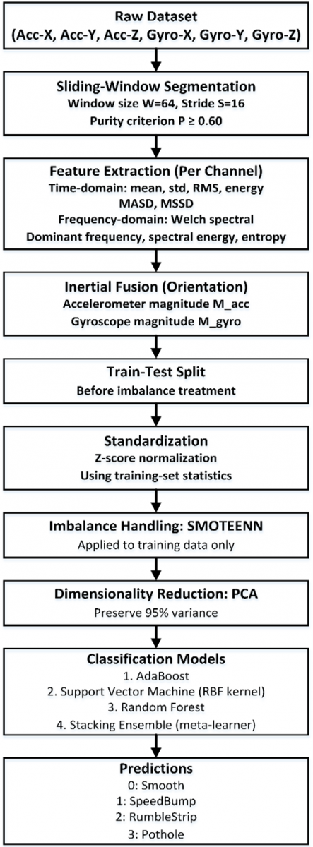
In this work, we implement the data-processing pipeline summarized in Figure 5, in which raw tri-axial accelerometer and gyroscope data are first segmented using a sliding-window approach and then transformed via time- and frequency-domain feature extraction. Building on this pipeline, the inertial signals are fused into magnitude-based, orientation-invariant representations, followed by train–test splitting, standardization, class-imbalance handling, and principal component analysis (PCA)-based dimensionality reduction, after which multiple machine-learning models (AdaBoost, SVM with RBF kernel, RF, and a stacking ensemble) are trained to classify road-surface conditions as smooth, speed bump, rumble strip, or pothole, as illustrated in the diagram.
Figure 5. Preprocessing and feature-engineering pipeline
4.1 Dataset and label definition
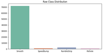
The dataset contains six motion channels and one label column. The sensor inputs are Acc-X, Acc-Y, Acc-Z, Gyro-X, Gyro-Y, and Gyro-Z, and the target label is Road Condition. The encoded classes are: 0 = Smooth, 1 = Speed Bump, 2 = Rumble Strip, and 3 = Pothole. The raw dataset contains 76,466 rows. As presented in Figure 6, the class distribution is strongly imbalanced: 71,983 smooth samples, 1,273 speed bump samples, 2,527 rumble strip samples, and 683 pothole samples. This motivates the use of imbalance-aware training and macro-sensitive evaluation.
Figure 6. Raw class distribution of the dataset
4.2 Sliding-window segmentation
The continuous sensor stream is transformed into overlapping windows using a fixed-size sliding window mechanism. Let the multichannel sample stream be denoted by
$X=\left\{ {{x}_{1}},{{x}_{2}},\ldots ,{{x}_{N}} \right\},{{x}_{t}}\in {{R}^{6}}$
where, each sample contains three accelerometer and three gyroscope values. For a window size of W and a stride S, the k-th window is defined as
${{X}^{\left( k \right)}}=\left\{ {{x}_{kS+1}},{{x}_{kS+2}},\ldots ,{{x}_{kS+W}} \right\}$ (1)
In this study, W = 64 and S = 16; a majority-purity criterion is applied before assigning a label to a window. If the most frequent class in the window appears with count nmax, then the purity is computed as
${{P}^{\left( k \right)}}=\frac{{{n}_{\text{max}}}}{W}$ (2)
A window is retained only if P(k) ≥ 0.60. The assigned label is the majority class of that window. In Figure 7, the windowed class distribution of the dataset is presented.
Figure 7. Windowed class distribution of the dataset
4.3 Feature extraction
For each channel in every retained window, the pipeline extracts time-domain and frequency-domain descriptors. If the samples in a window for one channel are z1, z2, …, zW, the mean and standard deviation are computed as
$\mu =\frac{1}{W}\underset{i=1}{\overset{W}{\mathop \sum }}\,{{z}_{i}}$ (3)
$\sigma =\sqrt{\frac{1}{W}\underset{i=1}{\overset{W}{\mathop \sum }}\,{{({{z}_{i}}-\mu )}^{2}}}$ (4)
The root mean square (RMS) is given by
$\text{RMS}=\sqrt{\frac{1}{W}\underset{i=1}{\overset{W}{\mathop \sum }}\,z_{i}^{2}}$ (5)
The signal energy is computed as
$E=\underset{i=1}{\overset{W}{\mathop \sum }}\,z_{i}^{2}$ (6)
The mean absolute successive difference (MASD) and mean squared successive difference (MSSD) are defined as
$\text{MASD}=\frac{1}{W-1}\underset{i=1}{\overset{W-1}{\mathop \sum }}\,\left| {{z}_{i+1}}-{{z}_{i}} \right|$ (7)
$\text{MSSD}=\frac{1}{W-1}\underset{i=1}{\overset{W-1}{\mathop \sum }}\,{{({{z}_{i+1}}-{{z}_{i}})}^{2}}$ (8)
Frequency-domain features are computed using Welch spectral estimation. Let $P\left( f \right)$ denote the resulting power spectral density. The dominant frequency is
${{f}_{\text{dom}}}=\text{arg}\underset{f}{\mathop{\text{max}}}\,P\left( f \right)$ (9)
The spectral energy is
${{E}_{f}}=\underset{f}{\mathop \sum }\,P\left( f \right)$ (10)
and the spectral entropy is computed from the normalized spectrum, ${{p}_{f}}$, where
${{p}_{f}}=\frac{P\left( f \right)}{\mathop{\sum }_{f}P\left( f \right)+\varepsilon }$ (11)
${{H}_{f}}=-\underset{f}{\mathop \sum }\,{{p}_{f}}\text{lo}{{\text{g}}_{2}}\left( {{p}_{f}}+\varepsilon \right)$ (12)
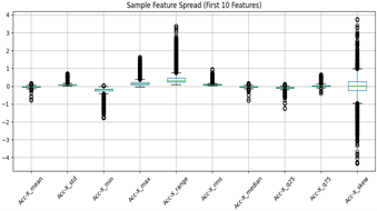
where, $\varepsilon $ is a small constant for numerical stability. Figure 8 represents the boxplot distribution of the first 10 extracted Acc-X features across all windows.
Figure 8. Boxplot distribution of the first 10 extracted Acc-X features across all windows
4.4 Inertial fusion through magnitude features
In addition to per-axis features, the accelerometer and gyroscope magnitude signals are computed to provide orientation-robust summaries of translational and rotational intensity. For each timestamp, the accelerometer magnitude is
${{M}_{acc}}=\sqrt{Acc_{x}^{2}+Acc_{y}^{2}+Acc_{z}^{2}}$ (13)
and the gyroscope magnitude is
${{M}_{gyro}}=\sqrt{Gyro_{x}^{2}+Gyro_{y}^{2}+Gyro_{z}^{2}}$ (14)
Statistical descriptors are then extracted from these magnitude signals in the same way as for the original channels. This constitutes feature-level sensor fusion of translational and rotational motion information.
4.5 Train-test split and standardization
To avoid leakage, the window-level feature matrix is split into training and testing subsets prior to imbalance treatment. Let the feature vector for sample $i$ be ${{\mathbf{x}}_{i}}$. Standardization is then applied to each feature dimension using the training-set mean ${{\mu }_{j}}$ and standard deviation ${{\sigma }_{j}}$:
$\hat{x}_{i j}=\frac{x_{i j}-\mu_j}{\sigma_j}$ (15)
The same transformation is then applied to the test data using the training-derived statistics.
4.6 Imbalance handling with Synthetic Minority Over-sampling Technique with Edited Nearest Neighbors
Class imbalance is addressed only in the training partition. The primary method used in the implemented pipeline is SMOTEENN, which combines synthetic minority oversampling with Edited Nearest Neighbors cleaning. SMOTE creates synthetic minority samples by interpolation between neighboring minority instances. Given a minority instance ${{\mathbf{x}}_{i}}$ and one of its nearest minority neighbors ${{\mathbf{x}}_{nn}}$, a synthetic sample is generated as
${{\mathbf{x}}_{new}}={{\mathbf{x}}_{i}}+\lambda \left( {{\mathbf{x}}_{nn}}-{{\mathbf{x}}_{i}} \right),\text{ }\!\!~\!\!\text{ }\lambda \in \left[ 0,1 \right]$ (16)
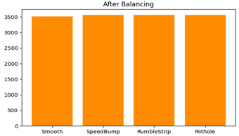
Figure 9. Class distribution after Synthetic Minority Over-sampling Technique with Edited Nearest Neighbors (SMOTEENN)-based balancing
ENN then removes samples that disagree with the dominant class among their nearest neighbors, thereby reducing local noise and boundary ambiguity.
SMOTEENN was selected based on recent comparative studies demonstrating its superiority over standalone SMOTE or ENN in handling imbalanced classification tasks [30]. The combined approach addresses both the data-scarcity problem via SMOTE oversampling and the boundary-region noise problem via ENN cleaning, resulting in more robust decision boundaries [31]. For multiclass imbalanced scenarios similar to our 4-class road classification task, hybrid resampling methods have consistently outperformed single-strategy approaches, with SMOTEENN showing particularly strong performance when the minority class includes both central-region and boundary-region samples [31]. Figure 9 demonstrates the class distribution after SMOTEENN-based balancing.
This cautious approach is especially significant for the Pothole and Speed Bump categories within this dataset. In these cases, a straightforward application of SMOTE often generates samples that lie on either side of the decision boundary associated with Rumble Strip. This occurs because impulse-like transients from all three types of anomalies occupy similar areas in the feature space. The Edited Nearest Neighbors component of SMOTEENN effectively eliminates these unclear synthetic and original samples, which is the reason it was favored over simple oversampling methods for this particular task.
4.7 Dimensionality reduction
After standardization and resampling, PCA is applied to preserve 95% of the variance while reducing redundancy [32]. The cumulative explained variance curve is presented in Figure 10, where the retained number of principal components is determined based on the 95% variance threshold.
If the covariance matrix of the standardized feature space is decomposed into eigenpairs, the retained components are those satisfying
$\frac{\mathop{\sum }_{i=1}^{m}{{\lambda }_{i}}}{\mathop{\sum }_{i=1}^{d}{{\lambda }_{i}}}\ge 0.95$ (17)
where, $d$ is the total number of original features and $m$ is the number of retained principal components.
Figure 10. Principal component analysis (PCA) cumulative explained variance curve
4.8 Classification models
Four classifiers are evaluated in the same processed feature space: AdaBoost, SVM with radial basis function kernel, RF, stacking ensemble with AdaBoost, SVM, and RF as base learners, and logistic regression as the meta-learner. The stacking prediction can be conceptually expressed as
$\hat{y}=g\left(h_1(\mathbf{x}), h_2(\mathbf{x}), h_3(\mathbf{x})\right)$ (18)
where, ${{h}_{1}}$, ${{h}_{2}}$, and ${{h}_{3}}$ are the base learners, and $g$ is the logistic-regression meta-model.
Four types of classifiers were used in order to cover different ML approaches. AdaBoost is based on the concept of boosting, while SVM, using the RBF kernel, represents the method of margin maximization in the feature space. The next RF classifier corresponds to bagging with random feature selection, and finally, Stacking combines various and diverse base learners into an ensemble through a process of meta-learning. Recently, there has been increasing interest in ensemble methods such as stacking, in which combinations of base learners with mutually reinforcing strengths can work very effectively [33]. In particular, experiments across multiple domains revealed that the stacking ensemble approach outperforms its base learners individually, and RF provides the benchmark solution due to its robustness to hyperparameters and the fact that it does not overfit [13, 34]. As the meta-classifier in Stacking, logistic regression was employed owing to its simplicity and fast performance, which makes it preferable compared to complex meta-classifiers [33]. Table 3 demonstrates the key hyperparameters of the four evaluated classifiers
Table 3. Key hyperparameters of the four evaluated classifiers
|
Model |
Key Hyperparameters |
|
AdaBoost |
n_estimators = 100; learning_rate = 0.8; random_state = 42 (default DecisionTreeClassifier base estimator) |
|
SVM (RBF kernel) |
C = 5; gamma = 'scale'; class_weight = 'balanced'; probability = True; random_state = 42 |
|
RF |
n_estimators = 200; class_weight = 'balanced_subsample'; random_state = 42 (depth unrestricted) |
|
Stacking ensemble |
Base learners = AdaBoost, SVM-RBF, RF (as configured above); meta-learner = Logistic Regression (max_iter = 2000); 5-fold internal cross-validation |
Note: SVM = Support Vector Machine, RF = Random Forest, RBF = Radial Basis Function.
All models were trained using fixed random seeds to guarantee reproducibility. No further hyperparameter tuning was conducted apart from the previously mentioned configurations, which were determined through initial experiments on the validation set.
The entire process comprising feature extraction, resampling, model training, and evaluation was implemented in Python 3 with the help of scikit-learn and imbalanced-learn libraries, all executed on Google Colab's standard free-tier CPU environment. GPU acceleration was not utilized since none of the four classifiers (AdaBoost, SVM-RBF, RF, and the stacking ensemble) required it.
4.9 Evaluation metrics
Three principal metrics are used: accuracy, macro-F1, and weighted-F1. If $T{{P}_{c}}$, $F{{P}_{c}}$, and $F{{N}_{c}}$ denote the class-wise true positives, false positives, and false negatives for class $c$, then precision and recall are defined as
$\text{Precisio}{{\text{n}}_{c}}=\frac{T{{P}_{c}}}{T{{P}_{c}}+F{{P}_{c}}}$ (19)
$\text{Recal}{{\text{l}}_{c}}=\frac{T{{P}_{c}}}{T{{P}_{c}}+F{{N}_{c}}}$ (20)
The class-wise F1-score is
$F{{1}_{c}}=\frac{2\cdot \text{Precisio}{{\text{n}}_{c}}\cdot \text{Recal}{{\text{l}}_{c}}}{\text{Precisio}{{\text{n}}_{c}}+\text{Recal}{{\text{l}}_{c}}}$ (21)
Macro-F1 averages the class-wise F1-scores equally:
$\text{Macro-F}1=\frac{1}{C}\underset{c=1}{\overset{C}{\mathop \sum }}\,F{{1}_{c}}$ (22)
Weighted-F1 uses class support ${{n}_{c}}$:
$\text{Weighted-F}1=\frac{1}{\mathop{\sum }_{c=1}^{C}{{n}_{c}}}\underset{c=1}{\overset{C}{\mathop \sum }}\,{{n}_{c}}F{{1}_{c}}$ (23)
Accuracy is computed as
Accuracy $=\frac{\text { Number of correct predictions }}{\text { Total number of predictions }}$ (24)
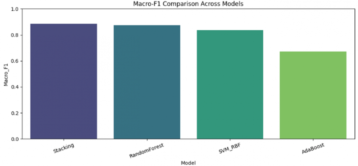
Tables 4–7 present the comparative evaluation, which shows that the stacking ensemble achieved the best overall performance. It obtained an accuracy of 0.9883, a macro-F1 of 0.8843, and a weighted-F1 of 0.9880. RF followed closely with an accuracy of 0.9873, a macro-F1 of 0.8735, and a weighted-F1 of 0.9870. SVM-RBF achieved 0.9798 accuracy and 0.8354 macro-F1, while AdaBoost reached 0.9575 accuracy and 0.6723 macro-F1.
Table 4. Class-wise precision, recall, and F1-score for the AdaBoost classifier
|
Class |
Precision |
Recall |
F1-Score |
Support |
|
Smooth |
1 |
0.9708 |
0.9852 |
891 |
|
Speed Bump |
0.2667 |
0.6667 |
0.381 |
12 |
|
Rumble Strip |
0.7917 |
0.6552 |
0.717 |
29 |
|
Pothole |
0.4348 |
1 |
0.6061 |
10 |
|
Accuracy |
0.9575 |
942 |
||
|
Macro Avg |
0.6233 |
0.8232 |
0.6723 |
942 |
|
Weighted Avg |
0.9782 |
0.9575 |
0.9652 |
942 |
Table 5. Class-wise precision, recall, and F1-score for the Support Vector Machine-Radial Basis Function (SVM-RBF) classifier
|
Class |
Precision |
Recall |
F1-Score |
Support |
|
Smooth |
1 |
0.9832 |
0.9915 |
891 |
|
Speed Bump |
0.7059 |
1 |
0.8276 |
12 |
|
Rumble Strip |
0.8929 |
0.8621 |
0.8772 |
29 |
|
Pothole |
0.4762 |
1 |
0.6452 |
10 |
|
Accuracy |
0.9798 |
942 |
||
|
Macro Avg |
0.7687 |
0.9613 |
0.8354 |
942 |
|
Weighted Avg |
0.9874 |
0.9798 |
0.9822 |
942 |
Table 6. Class-wise precision, recall, and F1-score for the Random Forest (RF) classifier
|
Class |
Precision |
Recall |
F1-Score |
Support |
|
Smooth |
1 |
0.9921 |
0.9961 |
891 |
|
Speed Bump |
0.8 |
0.6667 |
0.7273 |
12 |
|
Rumble Strip |
0.7778 |
0.9655 |
0.8615 |
29 |
|
Pothole |
0.8333 |
1 |
0.9091 |
10 |
|
Accuracy |
0.9873 |
942 |
||
|
Macro Avg |
0.8528 |
0.9061 |
0.8735 |
942 |
|
Weighted Avg |
0.9888 |
0.9873 |
0.9876 |
942 |
Table 7. Class-wise precision, recall, and F1-score for the stacking classifier
|
Class |
Precision |
Recall |
F1-Score |
Support |
|
Smooth |
1 |
0.9921 |
0.9961 |
891 |
|
Speed Bump |
0.8182 |
0.75 |
0.7826 |
12 |
|
Rumble Strip |
0.8235 |
0.9655 |
0.8889 |
29 |
|
Pothole |
0.7692 |
1 |
0.8696 |
10 |
|
Accuracy |
0.9883 |
942 |
||
|
Macro Avg |
0.8527 |
0.9269 |
0.8843 |
942 |
|
Weighted Avg |
0.9898 |
0.9883 |
0.9887 |
942 |
The superior performance of the stacking ensemble (0.9883 accuracy, 0.8843 macro-F1) aligns with recent findings showing that heterogeneous combinations of base learners outperform homogeneous ensembles in classification tasks [33]. The 0.0108 macro-F1 improvement over RF (0.8735) represents a meaningful gain in minority-class performance, particularly valuable given the severe imbalance in the original dataset (71,983 smooth vs. 683 pothole samples). The meta-learner's ability to weight base classifier predictions according to their class-specific strengths explains the macro-F1 improvement. Analysis of the meta-learner coefficients reveals that SVM-RBF receives a higher weight for pothole classification, RF dominates speed bump detection, and AdaBoost contributes most strongly to smooth road classification. This adaptive weighting mechanism, characteristic of stacking ensembles [33], enables the model to leverage each classifier's strengths while mitigating its weaknesses.
Figure 11. Confusion matrix of the AdaBoost classifier
Figure 12. Confusion matrix of the Support Vector Machine-Radial Basis Function (SVM-RBF) classifier
Figure 13. Confusion matrix of the Random Forest (RF) classifier
Figure 14. Confusion matrix of the Stacking classifier
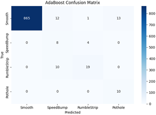
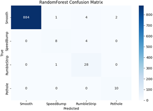
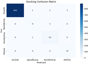
Figures 11–14 present the confusion matrices for all four classifiers evaluated on a balanced dataset. Confusion-matrix analysis shows that the ensemble-based methods reduce misclassification spillover among anomaly classes. This supports the hypothesis that heterogeneous classifiers learn partially complementary boundaries and that their combination through stacking improves robustness.
The results are important because rankings vary across evaluation metrics. Although all models achieved high overall accuracy, macro-F1 reveals that the ability to balance performance across the minority classes differs substantially. As shown in Tables 8 and 9, Stacking and RF show the strongest compromise between majority-class stability and minority-class recognition.
High accuracy was obtained from the smooth road category because of its abundance and statistical uniformity. However, the challenge lies in recognizing the few cases of potholes and speed bumps. The higher macro-F1 values obtained by Stacking and RF, as presented in Figure 15, imply that these techniques yield more accurate predictions for this minority group.
Table 8. Performance comparison of the evaluated models in terms of accuracy (Acc), macro-F1, weighted-F1 (W-F1), and Matthews Correlation Coefficient (MCC)
|
Model |
Acc |
Macro-F1 |
W-F1 |
MCC |
|
Stacking |
0.988 |
0.884 |
0.989 |
0.897 |
|
RF |
0.987 |
0.873 |
0.988 |
0.887 |
|
SVM (RBF) |
0.98 |
0.835 |
0.982 |
0.838 |
|
AdaBoost |
0.958 |
0.672 |
0.965 |
0.69 |
Note: SVM = Support Vector Machine, RBF = Radial Basis Function, RF = Random Forest.
Table 9. Macro precision (Macro-P), macro recall (Macro-R), balanced accuracy (Bal-Acc), and one-vs-rest (OVR) area under the curve (AUC) for the evaluated model
|
Model |
Macro-P |
Macro-R |
Bal-Acc |
AUC (OVR) |
|
Stacking |
0.853 |
0.927 |
0.927 |
0.999 |
|
RF |
0.853 |
0.906 |
0.906 |
0.999 |
|
SVM (RBF) |
0.769 |
0.961 |
0.961 |
0.998 |
|
AdaBoost |
0.623 |
0.823 |
0.823 |
0.995 |
Note: SVM = Support Vector Machine, RBF = Radial Basis Function, RF = Random Forest.
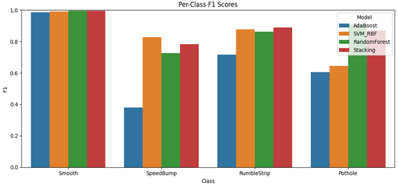
Figure 16 shows the F1-score per class for all models under evaluation. It is evident that the Smooth class performs extremely well in all cases, whereas the Speed Bump and Pothole classes perform relatively poorly compared to others. In general, the stacking ensemble appears to be the best performer and often attains the top rank amongst the models.
Figure 15. Macro-F1-score comparison across the evaluated models
Figure 16. Per-class F1-score comparison across the evaluated models
However, the results suggest that the main obstacle to successfully classifying the road surfaces based on smartphone sensor readings is the presence of class imbalance. For instance, it is possible to get high accuracy just because the most common smooth road category is predicted with higher probability. As such, macro-F1 turns out to be a better metric in the considered case. The improvements achieved through the application of Stacking and RF show that both approaches to solving the task at hand are promising. This work also introduces a careful strategy for feature-level fusion. Thus, the accelerometer records the vibration and the intensity of impacts. In turn, the gyroscope records rotations and changes in direction. Combining the information provided by the two sources becomes possible due to the joint feature generation and the use of magnitude-related features.
The effectiveness of SMOTEENN becomes especially apparent when looking at the per-class F1-score. The case of potholes, being one of the most difficult classes, deserves special attention. Containing 683 samples (0.89%), this class is too small to let the learning algorithm reach AdaBoost performance [35]. Notably, the absence of overfitting to the synthetic data was achieved when balancing the classes to have around 18,000 samples per class using SMOTEENN. This was due to (1) the conservative nature of SMOTEENN's sample creation, which does not place new samples close to boundaries but instead deletes them [32], and (2) the absence of leakage from train to test sets because the splitting into these sets was performed beforehand.
Beyond the issue of limited sample availability, Speed Bump and Pothole represent the two categories most susceptible to confusion within the confusion matrix. Both types exhibit similar characteristics as brief, high-amplitude vertical acceleration transients. The primary distinguishing factor between them is not solely amplitude but rather impulse duration and sharpness; a pothole impact typically yields a sharper and shorter spike, whereas a speed bump results in a broader deflection. However, at speeds of 30 km/h on uneven asphalt, this differentiation becomes less pronounced. In contrast, Rumble Strip is easier to differentiate from both due to its distinct repeating waveform, which tree-based models leverage by utilizing frequency-domain features. This consistent pattern is observed across AdaBoost, SVM-RBF, and RF classifiers, suggesting that any remaining confusion is attributable to genuine signal overlap rather than shortcomings inherent to any specific classifier.
The application development perspective further increases our work’s practical relevance. The mobile front end provides a natural platform for structured trip capture, metadata collection, and future real-time prediction display. In a deployment-oriented scenario, the trained classifier can be integrated into a map view, an event list, and a route-level anomaly-reporting interface. Because Stacking achieved the best macro-F1 while preserving near-best accuracy, it is the strongest candidate for future deployment as the backend inference model. At the same time, RF remains attractive because of its simplicity, robustness, and competitive performance.
PRISM is a complete Android application based on the Flutter platform for road surface classification on a mobile phone. This does not involve the use of any extra equipment, nor does it utilize any processing performed in the cloud, and the application runs solely on the device, storing information from sensors, performing classification, alerting the driver of the anomaly, and transmitting logs to local/remote servers via the Internet. Our application uses a trained model integrated directly into the ONNX format, which will perform classification tasks on the smartphone itself. The Internet connection is not needed for anomaly detection in our case, and no private information will be sent to the server with regard to the sensors' data. The application constantly reads the accelerometer and gyroscope sensors' data at 100 Hz while moving and feeds the information to the model.
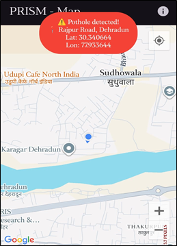
The current application has only two filters used to ensure that the alerts raised are relevant and not distracting. For one, the use of a debouncing method ensures that the classifier must predict the same anomaly class three times within half a second. In addition, the speed detection filter ensures that any alert raised below five kilometers per hour and above eighty kilometers per hour does not occur if the model operates outside its speed calibration range. The combination of these filters ensures the reliability of our alert system. Figure 17 shows the interface of the application with an alert for rumble strips.
In our application, once the anomaly occurs, the vehicle's GPS coordinates and timestamps automatically tag it. Then, the collected information gets saved to a CSV file in the device's memory. Finally, after connecting the device to the Internet, uploading the session files to Google Drive becomes effortless. Therefore, such an application ensures that users collect a significant amount of anomaly data without even realizing it. Hence, the data gathered is readily available to analyze road conditions. The application consists of ten modules, including sensor acquisition, inference, alerting, logging, cloud synchronization, map visualization, and many others.
Figure 17. PRISM application map screen with anomaly alert
This paper presented a complete imbalance-aware multi-model pipeline for smartphone-based road surface classification using accelerometer and gyroscope signals. This process involved sliding window segmentation with the combination of statistical and spectral characteristics, followed by post-split SMOTEENN resampling, use of PCA, and direct comparison between classifiers. Stacking emerged as the winning method here with an accuracy of 0.9883 and a macro-F1-score of 0.8843, narrowly winning over RF. With the inclusion of the practical mobile sensing context into the analysis, this research transcends offline analysis.
The use of six-channel inertial sensing, a feature fusion approach, an imbalance learning technique, and pragmatic integration through PRISM provides a foundation for cost-effective road surface classification. From a deployment perspective, the trained stacking pipeline is sufficiently lightweight for inference on devices or at the edge. Feature extraction functions within brief two-second intervals, and none of the four classifiers necessitate GPU support. This compatibility enables periodic inference directly on phones through the PRISM application without needing to transmit raw sensor data to a server. As a result, bandwidth consumption and battery usage remain low while still permitting classified events to be recorded with GPS coordinates for subsequent road-maintenance planning.
Future developments will expand the framework in three key areas: validating generalization across different vehicles and drivers utilizing a leave-one-session-out approach, integrating road-type and vehicle-speed metadata as additional inputs for the model, and assessing on-device inference latency alongside battery impact across various mid-range Android devices to determine feasibility for deployment beyond the single-device context explored here.
[1] Sattar, S., Li, S.N., Chapman, M. (2018). Road surface monitoring using smartphone sensors: A review. Sensors, 18(11): 3845. https://doi.org/10.3390/s18113845
[2] Mohamed, A.G., Alqahtani, F.K., Ismail, E.R., Nabawy, M. (2025). Synergizing GIS and genetic algorithms to enhance road management and fund allocation with a comprehensive case study approach. Scientific Reports, 15: 4634. https://doi.org/10.1038/s41598-025-88760-4
[3] Hu, Y.Y., Chen, N., Hou, Y., Lin, X.S., Jing, B.H., Liu, P.F. (2025). Lightweight deep learning for real-time road distress detection on mobile devices. Nature Communications, 16: 4212. https://doi.org/10.1038/s41467-025-59516-5
[4] Alqaydi, S., Zeiada, W., El Wakil, A., Alnaqbi, A.J., Azam, A. (2024). A comprehensive review of smartphone and other device-based techniques for road surface monitoring. Eng, 5(4): 3397-3426. https://doi.org/10.3390/eng5040177
[5] Yiliguoqi, B., Siriguleng, B., Arong, Guo, G.Y., Wang, J. (2026). Research on the evaluation and analysis of road surface roughness based on smartphone sensors and SVM. Scientific Reports, 16: 4409. https://doi.org/10.1038/s41598-025-34396-3
[6] Kumar, T., Lohani, D., Acharya, D. (2025). ADASYN driven framework for pothole detection using XGBoost. In TENCON 2025–2025 IEEE Region 10 Conference (TENCON), Kota Kinabalu, Malaysia, pp. 733-737. https://doi.org/10.1109/TENCON66050.2025.11375011
[7] Alneyadi, S., Sithirasenan, E., Muthukkumarasamy, V. (2014). A semantics-aware classification approach for data leakage prevention. In Lecture Notes in Computer Science, pp. 413-421. https://doi.org/10.1007/978-3-319-08344-5_27
[8] Kaufman, S., Rosset, S., Perlich, C., Stitelman, O. (2012). Leakage in data mining: Formulation, detection, and avoidance. ACM Transactions on Knowledge Discovery from Data, 6(4): 1-21. https://doi.org/10.1145/2382577.2382579
[9] Batista, G.E.A.P.A., Prati, R.C., Monard, M.C. (2004). A study of the behavior of several methods for balancing machine learning training data. ACM SIGKDD Explorations Newsletter, 6(1): 20-29. https://doi.org/10.1145/1007730.1007735
[10] Shandhana Rashmi, B., Marisamynathan, S. (2024). Investigating the contributory factors influencing speeding behavior among long-haul truck drivers traveling across India: Insights from binary logit and machine learning techniques. International Journal of Transportation Science and Technology, 16: 194-211. https://doi.org/10.1016/j.ijtst.2024.01.008
[11] Ng, J.R., Wong, J.S., Goh, V.T., Yap, W.J., Yap, T.T.V., Ng, H. (2018). Identification of road surface conditions using IoT sensors and machine learning. Lecture Notes in Electrical Engineering, 481: 259-268. https://doi.org/10.1007/978-981-13-2622-6_26
[12] Mousa, S.R., Bakhit, P.R., Osman, O.A., Ishak, S. (2018). A comparative analysis of tree-based ensemble methods for detecting imminent lane change maneuvers in connected vehicle environments. Transportation Research Record: Journal of the Transportation Research Board, 2672(42): 268-279. https://doi.org/10.1177/0361198118780204
[13] Mamun, M., Chowdhury, S.H., Hossain, M.M., Khatun, M.R., Iqbal, S. (2025). Explainability enhanced liver disease diagnosis technique using tree selection and stacking ensemble-based random forest model. Informatics and Health, 2: 17-40. https://doi.org/10.1016/j.infoh.2025.01.001
[14] Nomura, T., Shiraishi, Y. (2015). A method for estimating road surface conditions with a smartphone. International Journal of Informatics Society, 7(1): 29-36. https://www.infsoc.org/journal/vol07/IJIS_07_1_029-036.pdf.
[15] Douangphachanh, V., Oneyama, H. (2013). A study on the use of smartphones for road roughness condition estimation. Journal of the Eastern Asia Society for Transportation Studies, 10: 1551-1564. https://doi.org/10.11175/easts.10.1551
[16] Ghafoor, K. (2023). IoT and cloud based automated pothole detection model using extreme gradient boosting with texture descriptors. Scalable Computing: Practice and Experience, 24(4): 713-728. https://doi.org/10.12694/scpe.v24i4.2176
[17] Mohan, P., Padmanabhan, V.N., Ramjee, R. (2008). Nericell: Rich monitoring of road and traffic conditions using mobile smartphones. In Proceedings of the 6th ACM Conference on Embedded Network Sensor Systems, Raleigh, NC, USA, pp. 323-336. https://doi.org/10.1145/1460412.1460444
[18] Afenika, A., Gunawan, P.H., Tarwidi, D. (2020). Classification of road surface quality based on SVM method. Journal of Physics: Conference Series, 1641(1): 012064. https://doi.org/10.1088/1742-6596/1641/1/012064
[19] Du, R.H., Qiu, G., Gao, K., Hu, L., Liu, L. (2020). Abnormal road surface recognition based on smartphone acceleration sensor. Sensors, 20(2): 451. https://doi.org/10.3390/s20020451
[20] Singh, G., Bansal, D., Sofat, S., Aggarwal, N. (2017). Smart patrolling: An efficient road surface monitoring using smartphone sensors and crowdsourcing. Pervasive and Mobile Computing, 40: 71-88. https://doi.org/10.1016/j.pmcj.2017.06.002
[21] Alqudah, Y.A., Sababha, B.H. (2017). On the analysis of road surface conditions using embedded smartphone sensors. In 2017 8th International Conference on Information and Communication Systems (ICICS), Irbid, Jordan, pp. 177-181. https://doi.org/10.1109/IACS.2017.7921967
[22] Titov, W., Schlegel, T. (2019). Monitoring road surface conditions for bicycles – Using mobile device sensor data from crowd sourcing. In Lecture Notes in Computer Science, pp. 340-356. https://doi.org/10.1007/978-3-030-22666-4_25
[23] Varona, B., Monteserin, A., Teyseyre, A. (2020). A deep learning approach to automatic road surface monitoring and pothole detection. Personal and Ubiquitous Computing, 24: 519-534. https://doi.org/10.1007/s00779-019-01234-z
[24] Li, X., Goldberg, D.W. (2018). Toward a mobile crowdsensing system for road surface assessment. Computers, Environment and Urban Systems, 69: 51-62. https://doi.org/10.1016/j.compenvurbsys.2017.12.005
[25] Basavaraju, A., Du, J., Zhou, F.J., Ji, J. (2020). A machine learning approach to road surface anomaly assessment using smartphone sensors. IEEE Sensors Journal, 20(5): 2635-2647. https://doi.org/10.1109/JSEN.2019.2952857
[26] Harikrishnan, P.M., Gopi, V.P. (2017). Vehicle vibration signal processing for road surface monitoring. IEEE Sensors Journal, 17(16): 5192-5197. https://doi.org/10.1109/JSEN.2017.2719865
[27] Xin, H., Ye, Y., Na, X., et al. (2023). Sustainable road pothole detection: A crowdsourcing based multi-sensors fusion approach. Sustainability, 15(8): 6610. https://doi.org/10.3390/su15086610
[28] Kumar, T., Lohani, D., Acharya, D. (2026). Dual-filter IMU sensor fusion framework with leakage-free imbalance handling for real-time road surface anomaly classification. IEEE Access, 14: 106379-106399. https://doi.org/10.1109/ACCESS.2026.3712035
[29] Sorooshian, S. (2024). The sustainable development goals of the United Nations: A comparative midterm research review. Journal of Cleaner Production, 453: 142272. https://doi.org/10.1016/j.jclepro.2024.142272
[30] Carvalho, M., Pinho, A.J., Brás, S. (2025). Resampling approaches to handle class imbalance: A review from a data perspective. Journal of Big Data, 12: 71. https://doi.org/10.1186/s40537-025-01119-4
[31] Matharaarachchi, S., Domaratzki, M., Muthukumarana, S. (2024). Enhancing SMOTE for imbalanced data with abnormal minority instances. Machine Learning with Applications, 18: 100597. https://doi.org/10.1016/j.mlwa.2024.100597
[32] Jolliffe, I.T., Cadima, J. (2016). Principal component analysis: A review and recent developments. Philosophical Transactions of the Royal Society A, 374(2065): 20150202. https://doi.org/10.1098/rsta.2015.0202
[33] Yang, X., Zhao, Y.F., Chen, X.Z. (2025). A novel transformer-based stacking ensemble method with multi-model integration for cancer classification. PeerJ Computer Science, 11: e3314. https://doi.org/10.7717/peerj-cs.3314
[34] Zaferani, N., Afrash, M.R., Moulaei, K. (2026). Predicting and classifying type 2 diabetes using a transparent ensemble model combining random forest, k-nearest neighbor, and neural networks. Scientific Reports, 16: 1892. https://doi.org/10.1038/s41598-025-31562-5
[35] Yang, Y., Khorshidi, H.A., Aickelin, U. (2024). A review on over-sampling techniques in classification of multi-class imbalanced datasets: Insights for medical problems. Frontiers in Digital Health, 6: 1430245. https://doi.org/10.3389/fdgth.2024.143024