Mahmoud Baklizi | Mohammad Alkhazaleh | Issa Atoum | Musab Alzghoul* | Hamza Alshawabkeh
© 2026 The authors. This article is published by IIETA and is licensed under the CC BY 4.0 license (http://creativecommons.org/licenses/by/4.0/).
OPEN ACCESS
The Titanic passenger survival data is a common tabular benchmark for binary classification, but evaluation usually focuses on discrimination while missing data is treated as a preprocessing issue. This study is not primarily a prediction study: it uses the dataset as a transparent testbed for a reliability-oriented evaluation protocol, and reports what that protocol reveals when its claims are tested rather than assumed. A missingness-aware pipeline based on Histogram-based Gradient Boosting (HGB) is evaluated with the area under the receiver operating characteristic curve (AUC), probability-quality measures (Brier score, expected calibration error and reliability diagrams) and post-hoc calibration by Platt scaling and isotonic regression. Because the effects at stake are small relative to the sampling variability of 891 records, the primary repeated-evaluation results are averaged over ten independent stratified 5-fold assignments and compared by paired tests. Four findings follow. First, Platt scaling is strictly monotone and leaves within-fold AUC exactly unchanged, whereas isotonic regression can alter AUC only through the ties it introduces; the larger apparent gain attributed to calibration arises from the refitting performed inside the calibration wrapper rather than from the probability transformation itself. Second, isotonic calibration improves probability quality in all ten repetitions, reducing expected calibration error from 0.0643 to 0.0371, whereas Platt scaling improves the Brier score without a detectable effect on calibration error. Third, missingness indicators are informative in isolation but largely redundant once passenger class and fare are observed; removing those two variables makes them significantly useful again (AUC +0.0237, p = 0.002), and where the learner handles missing values natively, they become exactly redundant. Fourth, HGB outperforms six alternative learners on discrimination while three are better calibrated, and every class-imbalance resampling strategy tested degrades probability quality. Reliability and discrimination must therefore be reported and tested separately.
Brier score, expected calibration error, gradient boosting, informative missingness, probability calibration, tabular classification
The sinking of the Royal Mail Ship (RMS) Titanic on April 15, 1912, is one of the best-documented shipwrecks. The sinking of the ship, which carried some 2,224 passengers and crew, resulted in the deaths of over 1,500 people [1]. The Kaggle Titanic dataset, a mixture of passenger features and a binary survival outcome, has become a standard test case for machine learning practitioners working on binary classification problems with tabular data. While small, the dataset presents several modeling challenges like many real-world datasets: mixed (numeric and categorical) attributes, high levels of missingness, class imbalance, and the need to produce interpretable and robust predictions.
Many studies have investigated the prediction of Titanic survival with machine learning methods including logistic regression [2], decision tree [3], random forest [4, 5], k-nearest neighbor (KNN) [2], support vector machine (SVM) [6], and artificial neural network (ANN) [7]. These studies have contributed to gaining insights into the important factors affecting survival, such as sex, social class, age, fare, and family size. However, most of these have primarily focused on reporting accuracy-related measures such as accuracy, F1-score, or area under the receiver operating characteristic curve (AUC) while neglecting the quality of the probability estimates. In many applications of predictive modeling, the reliability of probabilities is crucial as well as discrimination [8, 9].
Two properties of the Titanic dataset motivate the reliability-oriented approach taken here. The first is the extent of its missing data: the cabin field is absent for 77.1% of passengers and age for 19.9%. The second is the size of the sample, 891 records, which makes the uncertainty of any performance estimate large relative to the differences typically reported. Together, these place the dataset in the regime where discrimination measures alone are least informative and where optimistic conclusions are easiest to reach.
Rather than proposing a new learner, this paper contributes an evaluation protocol and the findings it produces. Titanic is used as a case study because it combines jointly uncommon properties, as argued in Section 3.1. The contributions are:
(1). A methodological correction. Platt scaling cannot change the ranking of samples and therefore cannot change the AUC. We show that AUC differences reported for calibrated models arise from the internal resampling of the calibration wrapper rather than from calibration itself, and we quantify the two effects separately.
(2). An ablation-based treatment of informative missingness. We test, rather than assert, whether missingness indicators contribute predictive value, and find that they are informative but redundant with observed socio-economic variables. We give a reusable diagnostic for distinguishing the two cases.
(3). Reliability-oriented evaluation with explicit uncertainty. Probability quality is reported using the Brier score, expected calibration error (ECE), and reliability diagrams; all comparisons use paired bootstrap tests on metric differences rather than inspection of overlapping marginal intervals; and calibrator stability is measured across repeated resampling.
The rest of this paper is organized as follows. Section 2 discusses previous work on Titanic survival prediction, probability calibration, and strategies for dealing with missing data. Section 3 provides an overview of the proposed approach. Section 4 presents the results in terms of quantitative evaluation results, reliability diagrams, and a feature importance study. Section 5 discusses the results and their applications. Section 6 discusses threats to validity, and Section 7 concludes this paper and discusses directions for further research.
2.1 Machine learning for Titanic survival prediction
The Titanic data has been used as a test case for classification problems. Farag and Hassan [3] used the Kaggle data to train decision trees and Gaussian naïve Bayes and achieved 90.01% and 92.52% accuracy, respectively. They highlighted the need for feature selection and found sex to be a key predictor. They also found that including the Ticket feature in the model improved accuracy, and a small tree-based model with naïve Bayes achieved the best accuracy in their experiment.
Huang [4] applied a random forest model and examined the importance of features, finding that age, fare, and sex were the top three predictors of survival. They found an accuracy of 76.0% and touched on the historical significance of the features, such as the fare/passenger class - lifeboat relationship. Al-Hayik and Abu-Naser [7] applied ANN in the Jordan Neural Network (JNN) environment with 78% accuracy after 100 epochs of training, with age and sex as the most significant features.
Li [5] developed a hybrid method of combined feature engineering and ensemble-model optimization (logistic regression, random forest, XGBoost). The authors reported cross-validated accuracies from 0.8204 for XGBoost to 0.8361 for ensemble models, using various hyperparameter tuning approaches. The new features were generated from titles, cabins, and family connections.
Tree-based ensemble methods such as random forests and gradient-boosted trees are widely used for tabular classification because they capture nonlinear interactions and handle heterogeneous predictors effectively [10, 11]. Benchmarks continue to find them competitive with, or superior to, deep architectures on datasets of the scale considered in the study [12], although recent gradient-based tree ensembles narrow the gap [13]. Section 4.10 tests this choice on the present data rather than assuming it.
Li [2] compared the performance of logistic regression and the KNN algorithm, and found that logistic regression had greater accuracy (79.19%) than KNN (77.66%). Gender, status, and class were found to be the most important features for survival. Singh et al. [6] compared Naïve Bayes, decision tree, and SVM and found the significance of gender for predicting survival.
Kakde and Agrawal [14] also conducted exploratory data analysis and employed common machine learning techniques to predict survival on Titanic, further highlighting its role as a classic tabular classification benchmark dataset.
While these works offer valuable insights about predictors and the performance of algorithms on Titanic data, they have two drawbacks. First, they are mostly concerned with accuracy measures and seldom with probability calibration. Second, they usually neglect the treatment of missing values by deleting or imputing them, rather than explicitly modeling them. Our work overcomes these limitations by leveraging missingness-aware feature engineering, probability calibration, and uncertainty-aware reporting.
2.2 Probability calibration and reliability evaluation
Probability calibration transforms classifier predictions to yield better-calibrated probabilities [8, 9], and recent surveys give a systematic account of the available methods and of how calibration should be assessed [15, 16]. Ideally, the survival rate among passengers assigned a probability near 0.70 by a well-calibrated model should be close to 70%. The Brier score [17], the mean squared difference between predicted probabilities and binary outcomes, is a proper scoring rule that combines discrimination and calibration; because it conflates the two, Dimitriadis et al. [18] argued for reporting calibration, discrimination, and overall skill as separate diagnostics, which is the practice adopted here.
Platt [19] proposed the sigmoid transformation that fits a logistic model to map classifier scores to probabilities. Zadrozny and Elkan [20] introduced isotonic-regression calibration, which is a non-parametric method that calibrates in a monotonic manner. In a more comprehensive empirical study, Niculescu-Mizil and Caruana [8] demonstrated that several supervised classifiers (including boosted classifiers) produce probability estimates that can be improved with calibration.
Recently, there has been a focus on neural networks and probabilistic classifiers. Guo et al. [9] demonstrated that deep networks are frequently not well-calibrated, despite impressive accuracy. Naeini et al. [21] developed Bayesian Binning into Quantiles (BBQ), and Kull et al. [22] proposed beta calibration as an extension to logistic calibration. These advances highlight the need for calibration to be considered as a separate aspect of model assessment.
More recent work has explored trainable calibration measures for neural networks and probabilistic classifiers [23], and has examined the interaction between model selection and calibration, showing that the stopping and tuning decisions taken during fitting change how much a post-hoc calibrator can contribute [24]. This bears directly on the tuning ablation reported in Section 4.3.
2.3 Handling class imbalance and missing data in tabular classification
Aragão et al. [25] proposed a dynamic-balancing Automated Machine Learning (AutoML) framework that uses traditional and generative resampling techniques and dynamic thresholding for imbalanced tabular data. Their dataset benchmark included Titanic and 21 other datasets, and they demonstrated significant improvements in weighted F1-score for a number of cases. The Titanic dataset was described as moderate-complexity, low hardness, high-relevance data.
Classical resampling methods such as Synthetic Minority Over-sampling Technique (SMOTE) have been widely used to address class imbalance in supervised learning [26], although their effect on probability quality is less often examined; Section 4.8 measures it directly. On missing data, a growing body of work questions the value of elaborate imputation for prediction. Josse et al. [27] establish consistency results for supervised learning with missing values; Shadbahr et al. [28] report diminishing returns from improved imputation accuracy. Our Section 4.11 provides a limiting case: where the learner handles missing values natively, hand-engineered indicators are exactly redundant.
This suggests that our assumption that preprocessing, missing-data imputation, and class-distribution considerations can lead to better classification performance on Titanic-like tabular data is correct. This work continues in this vein but with a stronger emphasis on probability calibration, reliability assessment, and representation learning with an awareness of missingness, which have been less widely applied in Titanic survival analyses.
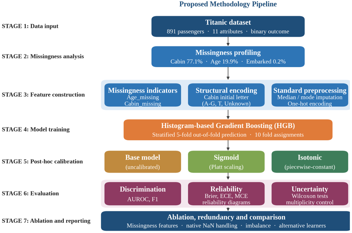
In this section, we present the proposed missingness-aware Histogram-based Gradient Boosting (HGB) pipeline, with post-hoc probability calibration. Our proposed approach is shown in Figure 1.
Figure 1. The methodology pipeline from data input through feature construction, model training and post-hoc calibration to the evaluation, ablation and redundancy analyses
3.1 Dataset description
We adopt the Titanic passenger survival data from Kaggle, which has 891 passenger records and a binary target variable Survived (0 = did not survive, 1 = survived). The classes are fairly balanced, with 549 (61.6%) non-survivors and 342 (38.4%) survivors. We have 11 descriptive attributes for each passenger: PassengerId, Pclass (ticket class: 1, 2 or 3), Name, Sex, Age, SibSp (number of siblings/spouses on board), Parch (number of parents/children on board), Ticket, Fare, Cabin and Embarked (port of embarkation: C, Q or S).
3.1.1 Justification for the choice of dataset
The Titanic dataset is a teaching benchmark, and its use in a research paper requires justification. We use it because it combines four properties that rarely occur together. Its missingness is extreme (77.10% for Cabin) and demonstrably non-random. The mechanism generating that missingness is historically documented rather than inferred, since cabin assignment followed ticket class and fare, so the informative-missingness hypothesis can be examined against a known cause instead of a statistical assumption.
The sample is small enough (891 records) that evaluation uncertainty is large relative to the effects under study, which is precisely the regime in which reliability-oriented reporting matters and in which optimistic conclusions are easiest to reach. Finally, the data are public and fixed, so every number in this paper can be reproduced exactly.
We state explicitly that we do not claim state-of-the-art predictive performance on this dataset, and that no such claim should be read into the comparisons in Section 5.3. The dataset is the instrument, not the object, of this study.
3.2 Missingness profile
A defining characteristic of these data is that several attributes contain values that are missing non-randomly. The missingness profile of all attributes is given in Table 1. Throughout this paper, the term missingness indicator refers to the binary variables Age_missing and Cabin_missing, and the term missingness-aware features refers to those indicators together with the categorical variable Cabin_letter; the distinction matters because Cabin_letter also encodes deck identity for recorded cabins and is therefore only partly a missingness feature.
The Cabin attribute has the highest missingness (77.10%), followed by Age (19.87%). Instead of considering these missing values as noise that can be imputed, this paper assumes that missingness may contain information on socioeconomic status, ticket, and cabin, which historically have been related to survival [1, 3].
Table 1. Missingness profile of the Titanic dataset
|
Attribute |
Missing Count |
Missing Percentage (%) |
|
Cabin |
687 |
77.10 |
|
Age |
177 |
19.87 |
|
Embarked |
2 |
0.22 |
|
Other attributes |
0 |
0.00 |
3.3 Missingness-aware feature engineering
To test the informative-missingness hypothesis, three features are constructed. Age_missing indicates whether age is absent. Cabin_missing indicates whether the cabin field is absent. Cabin_letter is a categorical variable holding the first letter of the cabin identifier (A, B, C, D, E, F, G or T), or Unknown when the field is empty. This retains the deck information available for recorded cabins while also representing the availability of the field itself. Section 4.6 evaluates each of the three separately.
The data preprocessing consists of the following steps. First, numerical attributes (Age, SibSp, Parch, Fare, and the missingness flags) are imputed with the median value and then z-score normalized. Second, categorical features (Sex, Embarked, Pclass, and Cabin_letter) are imputed with the most frequent category and encoded using one-hot encoding (untrained categories will be safely ignored at inference time). Third, these non-informative identifier fields (PassengerId, Name, Ticket, and the original Cabin string) are removed from the final set of features.
3.4 Learning algorithm: Histogram-based Gradient Boosting
The primary learning algorithm is the HGB classifier, using scikit-learn [29] (version 1.5) and similar to histogram-based gradient-boosting algorithms [30]. HGB breaks continuous features into histograms when growing trees, which increases the speed and makes it possible to perform repeated cross-validated experiments on diverse tabular data.
HGB was chosen because it suits heterogeneous tabular data, captures non-linear interactions, and is computationally efficient, which makes the repeated evaluation protocol of Section 3.5 feasible. Section 4.10 tests this choice against six alternatives under an identical protocol. The hyperparameters were left at the scikit-learn defaults for the main results, since the object of study is the evaluation protocol rather than peak predictive performance; Section 4.3 reports what tuning changes.
3.5 Evaluation protocol
To get accurate estimates of performance and avoid overfitting, we use stratified five-fold cross-validation. Stratification means that class proportions are maintained in each fold. The model is trained on four folds and tested on the remaining fold in each iteration. Once all folds are done, we have out-of-fold (OOF) predictions for all the instances, where each prediction is not based on the model that was trained with the instance itself.
Because the effects examined in this paper are small relative to the sampling variability of an 891-record dataset, a single fold assignment is not a sufficient basis for inference. Unless explicitly stated otherwise, every result reported below is obtained by repeating the complete OOF procedure over ten independent fold assignments (seeds 42 to 51) and reporting the mean with the standard deviation (SD) across those repetitions. Comparisons between configurations use the Wilcoxon signed-rank test on the ten paired differences. We adopted this protocol after observing that several conclusions drawn from a single fold assignment reversed under repetition; the point is documented in Section 6 as a finding rather than concealed as a method detail.
Three performance measures are computed. AUC quantifies the model's ability to rank survivors above non-survivors at all possible classification thresholds [31, 32]. F1-score is the harmonic mean of precision and recall at the default threshold of 0.5 and captures the model's performance at a single threshold. The Brier score [17] is defined as
$B S=\frac{1}{N} \sum\left(p_i-y_i\right)^2$
where, pi is the predicted probability, and yi is the binary outcome; a lower value is better.
3.6 Post-hoc probability calibration
Two post-hoc calibration techniques are used to bring predicted probabilities closer to observed frequencies. Platt scaling, also known as sigmoid calibration [19], applies a parametric logistic transformation to the raw classifier scores and suits a miscalibration that is approximately sigmoidal. Isotonic regression [20] fits a non-parametric, monotonic, piecewise-constant function. It is the more flexible of the two but may overfit when the calibration set is small, a concern examined empirically in Section 4.9. Both are monotonic, which has a consequence for discrimination that is developed in Section 4.2.
Both of these calibration approaches are implemented in CalibratedClassifierCV in scikit-learn, using cross-validated calibration on the training folds. The OOF predictions are then used to evaluate the calibration, so that the evaluation of the calibrated and uncalibrated models is performed in the same unbiased way.
3.7 Uncertainty estimation via bootstrap confidence intervals
In order to report statistical uncertainty in the metrics, 95% bootstrap confidence intervals are obtained for 2,000 bootstrap resamples of the OOF predictions [33]. The AUC, F1-score, and Brier score are recomputed for each resample, and the 2.5th and 97.5th percentiles are taken as the confidence-interval bounds. This allows robust reporting of performance with uncertainty, without making strong assumptions about the distributions of the metrics.
4.1 Overall performance and calibration analysis
Table 2 reports the base HGB model and its calibrated variants under OOF prediction, averaged over ten-fold assignments with SD. Alongside the measures used previously, we report the ECE, because the Brier score conflates calibration with discrimination and the two can move differently.
Table 2. Histogram-based Gradient Boosting (HGB) performance with calibration (out-of-fold (OOF), mean and standard deviation (SD) over ten-fold assignments)
|
Method |
AUC (SD) |
F1 (SD) |
Brier Score (SD) |
ECE (SD) |
|
Base (uncalibrated) |
0.8672 (0.0052) |
0.7597 (0.0115) |
0.1361 (0.0036) |
0.0643 (0.0056) |
|
Platt scaling |
0.8706 (0.0064) |
0.7626 (0.0090) |
0.1323 (0.0026) |
0.0604 (0.0092) |
|
Isotonic calibration |
0.8654 (0.0082) |
0.7554 (0.0083) |
0.1313 (0.0033) |
0.0371 (0.0063) |
Averaged over ten-fold assignments, the base model attains an AUC of 0.8672 (SD 0.0052), an F1-score of 0.7597 (0.0115), a Brier score of 0.1361 (0.0036) and an ECE of 0.0643 (0.0056). We note that the single fold assignment used in the earlier version of this work (seed 42) returned an AUC of 0.8787, near the top of the observed range, which illustrates why the repeated protocol was adopted.
Both calibrators improve the Brier score, isotonic by 0.0047 (better in 10 of 10 repetitions, p = 0.002) and Platt scaling by 0.0037 (9 of 10, p = 0.004). On the ECE, the two separate clearly: isotonic reduces it by 0.0272, from 0.0643 to 0.0371, in every repetition (p = 0.002), whereas the Platt-scaling reduction of 0.0039 is not distinguishable from zero (8 of 10, p = 0.275). The ordering by Brier score therefore does not reproduce the ordering by calibration error, and a practitioner selecting a calibrator on Brier score alone would treat the two as near-equivalent when they are not.
The apparent gain of Platt scaling on AUC (+0.0033, 9 of 10, p = 0.014) is not a calibration effect; Section 4.2 shows it to be a consequence of the resampling performed inside the calibration wrapper. Under Bonferroni correction across the 21 tests reported in this paper, the two isotonic results survive (adjusted p = 0.042) while the Platt-scaling Brier score and AUC results do not; all four survive control of the false discovery rate at 5%. We report both adjustments rather than selecting the more favorable one.
4.2 Discrimination is invariant under strictly monotone calibration
Platt scaling is a strictly monotonic transformation of the classifier score and therefore preserves the ordering of samples exactly; AUC, which depends only on that ordering, must be unchanged. Isotonic regression is only weakly monotonic, so the ties it introduces can move AUC in either direction, though only slightly. Any reported increase in AUC following calibration must therefore originate elsewhere.
We verified this by applying both calibrators to an identical frozen base model within each fold. The within-fold AUC under Platt scaling is identical to the uncalibrated value in all five folds, to machine precision, with a Spearman correlation of 1.000000 between raw and calibrated scores. Isotonic calibration moves AUC by at most 0.0092 in either direction (it loses AUC in four folds and gains 0.0008 in the fifth), entirely explained by the roughly 155 ties it creates per fold. Table 3 reports the within-fold values.
The source of the apparent gain is the calibration wrapper. CalibratedClassifierCV with an internal three-fold scheme refits the base estimator on each internal fold and averages the outputs, so the object evaluated as the calibrated model is a three-member ensemble. Separating the two effects shows that a three-fold ensemble with no calibration reaches AUC 0.8816, a gain of +0.0029 over the single model, while adding Platt scaling on top changes AUC by +0.0001 (95% CI [–0.0020, +0.0020]). The discrimination movement belongs to the ensembling, not to the calibration.
One residual subtlety is worth recording. When OOF predictions are pooled across folds, each fold contributes a different monotone map, so the pooled AUC is not strictly invariant even for prefit models; in our experiments this accounts for a shift of below 0.001. Within any single fold, the invariance is exact.
Table 3. Within-fold AUC under monotone calibration applied to the same frozen base model
|
Fold |
AUC (Raw) |
AUC (Platt) |
AUC (Isotonic) |
Spearman |
Ties Added |
|
1 |
0.914032 |
0.914032 |
0.904875 |
1.000000 |
154 |
|
2 |
0.897059 |
0.897059 |
0.888636 |
1.000000 |
166 |
|
3 |
0.819051 |
0.819051 |
0.817580 |
1.000000 |
157 |
|
4 |
0.847193 |
0.847193 |
0.839171 |
1.000000 |
155 |
|
5 |
0.865510 |
0.865510 |
0.866308 |
1.000000 |
155 |
4.3 Hyperparameter tuning ablation
The submitted version of this paper reported a tuning ablation whose search shared folds with the reported evaluation. That table has been recomputed under a nested design. Within each outer training fold, a grid search over the learning rate {0.03, 0.05, 0.1}, the number of boosting iterations {100, 200, 300}, the maximum number of leaf nodes {15, 31, 63} and the L2 regularization {0, 1} is run on an inner three-fold split. Only the selected configuration is applied to the held-out outer fold. Model selection therefore cannot influence the reported OOF predictions. Table 4 supersedes the values given previously.
Table 4. Histogram-based Gradient Boosting (HGB) hyperparameter tuning ablation under nested cross-validation
|
Configuration |
AUC |
F1 |
Brier Score |
ECE |
|
Default HGB |
0.8787 |
0.7795 |
0.1284 |
0.0565 |
|
Tuned HGB |
0.8792 |
0.7827 |
0.1226 |
0.0500 |
|
Tuned + Platt |
0.8797 |
0.7783 |
0.1250 |
0.0544 |
|
Tuned + isotonic |
0.8787 |
0.7747 |
0.1222 |
0.0431 |
Unlike the other tables, this ablation was run on a single fold assignment because of the cost of the nested search; it should be read as indicative.
Under the nested protocol, tuning has a negligible effect on discrimination (AUC +0.0004, 95% CI [–0.0069, +0.0075], p = 0.911) but a significant effect on probability quality: the Brier score falls by 0.0058 ([–0.0114, –0.0005], p = 0.036). Applying either calibrator on top of the tuned model produces no further detectable change (Platt scaling, Brier score +0.0024, p = 0.270; isotonic, –0.0005, p = 0.847). This reverses the conclusion drawn in the earlier version of this work. On a dataset of this size, tuning the base learner and post-hoc calibration address overlapping deficiencies, and tuning should be attempted first.
4.4 Reliability diagrams
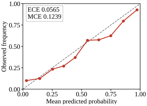
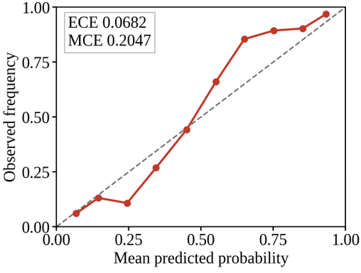
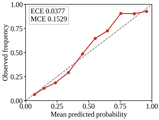
The reliability diagrams in Figures 2–4 are for the uncalibrated and calibrated models. The dashed diagonal line in each diagram indicates perfect calibration (predicted probabilities equal observed survival frequencies).
Figure 2. Reliability diagram for the base (uncalibrated) Histogram-based Gradient Boosting (HGB) model, annotated with expected calibration error (ECE) and maximum calibration error (MCE)
Figure 4. Reliability diagram after isotonic calibration, which tracks the diagonal most closely
The reliability diagrams refine rather than merely confirm Table 2. The panels are drawn from a single fold assignment and are illustrative; the numerical claims rest on the ten repetitions. Figure 2 shows the uncalibrated model deviating from the diagonal mainly in the mid-probability range. Figure 3 shows Platt scaling removing the local irregularity while displacing the curve upward, so survival is over-predicted across much of the range; averaged over repetitions, its net effect on the ECE is small and not distinguishable from zero. Figure 4 shows isotonic calibration tracking the diagonal most closely, consistent with the ECE reduction of 0.0272 observed in every repetition. Each panel is annotated with its ECE and maximum calibration error (MCE) for that fold assignment.
4.5 Feature importance analysis
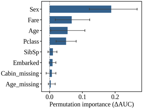
Permutation importances are reported as the change in AUC when a variable is shuffled. Two refinements were necessary. First, all encoded columns derived from the same original variable are permuted together with a common row permutation; permuting one-hot columns individually understates a variable, because the remaining columns of the same variable still carry its information. Second, the computation is repeated inside every fold with 20 repeats, and Figure 5 reports the mean with a 95% interval over the resulting estimates.
Four variables have intervals excluding zero: sex (mean ΔAUC 0.1880, [0.1214, 0.2670]), fare (0.0673, [0.0176, 0.1224]), age (0.0549, [0.0035, 0.1078]) and passenger class (0.0504, [0.0201, 0.0810]). Grouping raises passenger class from 0.0419 to 0.0504 and embarkation port from 0.0034 to 0.0092 relative to the per-column analysis, confirming that the per-column form understates categorical variables. The missingness-derived features remain indistinguishable from zero: Cabin_missing at 0.0069 ([–0.0105, 0.0193]), Age_missing at 0.0035 ([–0.0037, 0.0171]) and Cabin_letter at 0.0002 ([–0.0067, 0.0062]).
A caution is in order about how this figure should be read. Permutation importance measures how much a fitted model relies on a variable, not how much is gained by supplying it. The two can disagree in either direction, and they do here: Cabin_letter has essentially zero permutation importance yet contributes a small but consistent gain in the ablation of Section 4.6. We therefore use the ablation, not this figure, to decide whether a feature earns its place.
4.6 Ablation of the missingness-aware features
The informative-missingness hypothesis is tested by removing each engineered feature and measuring the effect over ten-fold assignments. Configuration M0 carries no missingness information at all: the Cabin column is dropped without replacement, and no indicator is created. Table 5 reports the ablation.
Table 5. Ablation of the missingness-aware features (out-of-fold (OOF), uncalibrated Histogram-based Gradient Boosting (HGB))
|
Configuration |
Features |
AUC (SD) |
Brier Score |
ΔAUC vs. M0 |
p |
|
M0 |
No missingness features |
0.8657 (0.0064) |
0.1365 |
- |
- |
|
M1 |
+ Age_missing |
0.8656 (0.0058) |
0.1364 |
–0.0001 |
0.846 |
|
M2 |
+ Cabin_missing |
0.8678 (0.0047) |
0.1360 |
+0.0021 |
0.020 |
|
M3 |
+ Cabin_letter |
0.8681 (0.0045) |
0.1354 |
+0.0024 |
0.020 |
|
M4 |
+ Age_missing + Cabin_missing |
0.8671 (0.0051) |
0.1361 |
+0.0014 |
0.105 |
|
M5 |
All three (proposed) |
0.8672 (0.0052) |
0.1361 |
+0.0015 |
0.131 |
The pattern is one of small, partly inconsistent gains. Two single-feature configurations improve on M0 by roughly 0.002 AUC in 8 of 10 repetitions (M2 and M3, both p = 0.020 uncorrected). Neither survives Bonferroni correction across the tests reported in this paper. The full combination proposed in the earlier version of this work is not distinguishable from M0 (+0.0015, p = 0.131). The features are therefore redundant with one another as well: adding all three yields less than adding either M2 or M3 alone. We record that on the single-fold assignment used previously, M0 appeared marginally the strongest configuration and the effect appeared absent altogether, which is the clearest illustration in this paper of why the repeated protocol is necessary.
4.7 Why the ablation fails: Redundancy with observed variables
A null ablation admits two explanations: the missingness pattern carries no signal, or it carries signal that is already available elsewhere. These are distinguishable, and the distinction matters for any system that might rely on missingness indicators.
The missingness pattern is strongly associated with the observed socio-economic variables. The probability that the cabin is unrecorded rises from 18.5% in first class to 91.3% in second and 97.6% in third (chi-square 557.3, p < 1e−100, Cramer's V = 0.791). The median fare is 55.22 when the cabin is recorded against 10.50 when it is not (Mann-Whitney p < 1e−50). Survival differs accordingly, at 66.7% against 30.0%, and the association survives stratification by class (odds ratios 0.46, 0.18 and 0.31 in first, second and third class, with p = 0.030, 0.007 and 0.079). Table 6 sets out the two arms of this test.
Table 6. Testing whether missingness is uninformative or informative but redundant
|
Test |
Result |
|
Cabin_missing against Pclass |
Cramer's V = 0.791, p < 1e−100 |
|
Median fare, cabin recorded vs. missing |
55.22 vs. 10.50, p < 1e−50 |
|
Survival, cabin recorded vs. missing |
66.7% vs. 30.0% |
|
Model using missingness features only |
AUC = 0.6426 |
|
Pclass and Fare removed: no indicators |
AUC = 0.8123 |
|
Pclass and Fare removed: indicators only |
AUC = 0.8360, gain +0.0237, 10/10, p = 0.002 |
|
Pclass and Fare removed: Cabin_letter only |
AUC = 0.8340, gain +0.0217, 10/10, p = 0.002 |
|
Pclass and Fare removed: all three |
AUC = 0.8336, gain +0.0213, 10/10, p = 0.002 |
The pattern is genuinely informative. A model using the missingness features alone reaches an AUC of 0.6426. The decisive test is what happens when the variables that duplicate the information are withheld: with passenger class and fare removed, the binary indicators alone raise AUC from 0.8123 to 0.8360, a gain of +0.0237 in every one of ten repetitions (p = 0.002). We separate the arms because Cabin_letter encodes deck identity for recorded cabins and is therefore partly a content feature; supplied alone it yields a comparable +0.0217, and supplying all three yields +0.0213, no more than either alone. The indicators and the deck encoding are substitutes, and the gain is not an artifact of the content feature.
Missingness in this dataset is thus informative but redundant. The indicators carry roughly 0.023 AUC of socio-economic signal, of which the observed class and fare variables absorb around nine tenths, leaving the residual 0.002 measured in Section 4.6. The practical consequence is conditional rather than universal: missingness indicators are worth engineering when the variables that would otherwise carry the same information are unobserved, unreliable or excluded by policy, and are not worth engineering when those variables are present and well measured. The test is inexpensive and generalizes to any dataset.
4.8 Class imbalance
The dataset is moderately imbalanced, with 61.6% non-survivors against 38.4% survivors. Because this paper evaluates probabilities rather than labels alone, imbalance handling is assessed on calibration as well as on discrimination. Table 7 summarizes the outcome.
Every strategy tested degrades probability quality in all ten repetitions. The Brier score worsens in 10 of 10 for each of the three (p = 0.002), as does the ECE, and both results survive Bonferroni correction. No strategy improves F1 significantly, and random oversampling and SMOTE significantly reduce AUC (9 of 10, p = 0.006 and p = 0.004). The mechanism is visible in the final column: resampling alters the class prior of the training sample, so the model no longer estimates the conditional probability on the original population, and the mean prediction drifts from the base rate of 0.3838 to between 0.40 and 0.41. Threshold moving attains a comparable F1 while leaving the probabilities untouched, and is therefore preferable whenever the probabilities themselves are consumed downstream.
Table 7. Imbalance handling
|
Strategy |
AUC |
F1 |
Brier Score |
ECE |
Mean Pred. |
|
None (proposed) |
0.8672 |
0.7597 |
0.1361 |
0.0643 |
0.3805 |
|
Class_weight = balanced |
0.8670 |
0.7622 |
0.1397 |
0.0821 |
0.4120 |
|
Random oversampling |
0.8644 |
0.7569 |
0.1424 |
0.0850 |
0.4009 |
|
SMOTE |
0.8633 |
0.7551 |
0.1417 |
0.0814 |
0.4018 |
4.9 Stability of the calibrators
Isotonic regression is non-parametric and may overfit a small calibration set. To measure this, the entire OOF procedure was repeated over ten independent resampling seeds at three calibration-set sizes, controlled through the number of internal folds.
The concern is partly justified. Isotonic regression is less stable than Platt scaling on the Brier score, and its relative instability grows as the calibration set shrinks, with standard-deviation ratios of 1.27, 1.30 and 1.55 at 237, 142 and 71 calibration samples. On ECE, however, isotonic regression is the more stable of the two.
Table 8. Run-to-run variability of each calibrator over ten resampling seeds
|
Calibration Set |
Method |
Brier Score Mean |
Brier Score SD |
ECE Mean |
ECE SD |
|
- |
Uncalibrated |
0.1361 |
0.0036 |
0.0643 |
0.0056 |
|
237 |
Platt |
0.1323 |
0.0026 |
0.0604 |
0.0092 |
|
237 |
Isotonic |
0.1313 |
0.0033 |
0.0371 |
0.0063 |
|
142 |
Platt |
0.1316 |
0.0023 |
0.0553 |
0.0091 |
|
142 |
Isotonic |
0.1303 |
0.0030 |
0.0373 |
0.0078 |
|
71 |
Platt |
0.1334 |
0.0022 |
0.0562 |
0.0117 |
|
71 |
Isotonic |
0.1314 |
0.0034 |
0.0392 |
0.0081 |
Its improvement is also more consistent than the single-fold analysis of Section 4.1 suggests. Isotonic calibration reduced the Brier score in all ten-fold assignments and the ECE in all ten (Wilcoxon signed-rank p = 0.002 for both), against nine and eight of ten for Platt scaling (p = 0.004 and p = 0.275). The mean reductions for isotonic regression are 0.0047 in Brier score and 0.0272 in ECE, the latter a 42% relative improvement. We note that the three calibration-set sizes in Table 8 are not independent replicates, since they reuse the same ten-fold assignments on the same 891 records; the evidence for consistency rests on ten paired observations, not thirty.
4.10 Comparison with other tabular learners
The choice of HGB is tested rather than asserted. Six alternatives were trained under identical preprocessing, folds, and seed, and compared on discrimination and probability quality. Table 9 reports the comparison.
Table 9. Comparison of learners under an identical evaluation protocol
|
Model |
AUC |
F1 |
Brier Score |
ECE |
|
Gaussian Naïve Bayes |
0.7806 |
0.6925 |
0.2363 |
0.2192 |
|
Extra trees |
0.8365 |
0.7124 |
0.1647 |
0.1166 |
|
KNN |
0.8466 |
0.7224 |
0.1456 |
0.0453 |
|
SVM (RBF kernel) |
0.8481 |
0.7464 |
0.1392 |
0.0271 |
|
Logistic regression |
0.8503 |
0.7366 |
0.1421 |
0.0410 |
|
Random forest |
0.8592 |
0.7289 |
0.1422 |
0.0701 |
|
HGB (proposed) |
0.8672 |
0.7597 |
0.1361 |
0.0643 |
HGB outperforms all six alternatives on AUC in 10 of 10 repetitions (p = 0.002 in every case, all surviving Bonferroni correction), and likewise on the Brier score. The calibration picture is the opposite, and it is the more instructive of the two. Three simpler models are better calibrated than HGB in all ten repetitions: the Radial Basis Function (RBF) SVM (ECE 0.0271 against 0.0643), logistic regression (0.0410), and KNN (0.0453), each with p = 0.002 and each surviving correction. The model that ranks best is thus among the worst calibrated, and a selection procedure that observes only discrimination will systematically choose a system whose probabilities are less trustworthy than those of alternatives it rejects.
4.11 Native missing-value handling
One arm was absent from the earlier version of this work and is decisive for its central question. HistGradientBoosting handles missing values natively, learning at each split the branch to which they are routed. The proposed pipeline imputes the median first, discarding that capability, and then reconstructs part of it by hand through binary indicators. Table 10 contrasts the two arms.
Table 10. Native missing-value handling against median imputation, ten-fold assignments
|
Arm |
Configuration |
AUC (SD) |
Brier Score |
ECE |
|
N0 |
Median imputation, no indicators |
0.8681 (0.0045) |
0.1354 |
0.0639 |
|
N1 |
Native NaN, no indicators |
0.8673 (0.0058) |
0.1362 |
0.0632 |
|
N2 |
Native NaN + indicators |
0.8673 (0.0058) |
0.1362 |
0.0632 |
|
N3 |
Median imputation + indicators |
0.8672 (0.0052) |
0.1361 |
0.0643 |
Arms N1 and N2 produce identical predictions in every repetition. This is not a numerical coincidence: Cabin_missing is by construction identical to the indicator Cabin_letter = Unknown, and Age_missing is identical to the missingness of Age, which the learner already exploits. When the model handles missingness natively, the engineered indicators are exactly redundant, and the trees are unchanged. Neither native handling nor the proposed pipeline improves on plain median imputation without indicators (N0), which attains the highest AUC of the four arms.
5.1 Discrimination versus reliability
The central distinction of this study is between discrimination and reliability. The uncalibrated HGB model ranks well (AUC 0.8672) while assigning probabilities that deviate from observed survival frequencies (ECE 0.0643), which is consistent with the calibration literature [8, 9]. The two properties are not merely different in degree. Section 4.10 shows three models that rank worse than HGB yet are better calibrated than it in every repetition, so no ordering of models by discrimination can be assumed to carry over to reliability.
The two calibrators differ in the flexibility they bring. Platt scaling fits a two-parameter logistic transformation and can correct a globally sigmoidal distortion but not a locally irregular one; averaged over ten-fold assignments, it lowers the Brier score by 0.0037 while its effect on the ECE (–0.0039) cannot be distinguished from zero. Isotonic regression fits a piecewise-constant monotone function, follows the observed distortion more closely, and lowers both by 0.0047 in Brier score and 0.0272 in ECE, in every repetition. The two measures therefore rank the calibrators differently in strength if not in sign, which is the practical argument for reporting a calibration-specific measure alongside the Brier score. Neither calibrator improves discrimination, and Platt scaling cannot: as established in Section 4.2, a strictly monotone transformation cannot alter the ranking on which AUC depends, whereas isotonic regression can move it only through the ties it introduces.
The evidence about calibration is best stated as a distinction between magnitude and direction. On any one-fold assignment, the improvement is small relative to the sampling uncertainty attached to 891 records, and a paired bootstrap on that single assignment does not reach significance. Across ten independent fold assignments, isotonic calibration improves both probability measures every time. These answer different questions: the first asks how large the effect would be on a new sample of this size, and the answer is that it cannot be pinned down; the second asks whether the procedure reliably moves in the right direction, and the answer is that it does. We claim only the second, and we note that the earlier version of this work reported a single-assignment result as though it settled the first.
The tuning ablation of Section 4.3 adds a further qualification. Tuning the base learner significantly improves the Brier score (p = 0.036), and once the model is tuned, neither calibrator produces a further detectable gain. On problems of this size, the deficiency that post-hoc calibration repairs is partly the same deficiency that hyperparameter selection repairs, and the simpler intervention should be tried first. This reverses the position taken in the earlier version of this work, which attributed the reliability gain to calibration after concluding that tuning was not responsible for it.
5.2 Informative missingness
A large proportion of the Cabin field is missing (77.1%), and prior studies generally handle this by deletion, imputation, or simplified encoding [2-7]. The submitted version of this paper concluded from permutation importance that the missingness was informative. Sections 4.5 to 4.7 show that this conclusion was not supported by the evidence offered for it: once uncertainty is attached to the importance estimates, the missingness features are indistinguishable from zero, and a direct ablation finds no benefit from adding them to the full feature set.
The revised conclusion is more specific. Missingness here is informative but redundant. Cabin recording followed ticket class and fare, so the indicators largely restate variables that are fully observed. When those variables are withheld, the indicators recover +0.0237 AUC in every repetition (p = 0.002). When they are present, the residual contribution falls to roughly 0.002 and no longer survives correction for multiple testing. Section 4.11 sharpens the point further: where the learner handles missing values natively, the engineered indicators are exactly redundant and leave the predictions unchanged. Informativeness and incremental value are therefore separate properties, and a permutation-importance plot measures neither reliably, since it reports what a fitted model uses rather than what the analyst gains by supplying a feature.
5.3 Comparison with prior work
Table 11 situates this work among previous Titanic studies. The comparison is contextual and not a benchmark: the studies cited differ in preprocessing, in the construction of their train and test splits, in whether cross-validation is used at all, and in the metrics reported. Accuracy figures obtained under different protocols are not commensurable, and we draw no superiority claim from them. Our own accuracy under stratified five-fold OOF evaluation is 0.8361, given for completeness rather than for ranking. The only comparative claims made in this paper are those of Section 4.10, where every model was trained by us under an identical protocol and differences were tested.
Table 11. Comparison with prior Titanic studies (N/R denotes not reported)
|
Study |
Algorithm |
Accuracy |
Calibration |
|
Li [2] |
Logistic Regression |
79.19% |
No |
|
Farag and Hassan [3] |
naïve Bayes |
92.52% |
No |
|
Huang [4] |
random forest |
76.0% |
No |
|
Li [5] |
Ensemble (Stacking) |
83.61% |
No |
|
Al-Hayik and Abu-Naser [7] |
ANN (JNN) |
78.0% |
No |
|
Aragao, et al. [25] |
AutoGluon + ADASYN |
N/R |
No |
|
This work |
HGB + post-hoc calibration |
83.61% (OOF) |
Yes |
5.4 Practical implications
The evidence in this paper comes from one historical dataset, and we therefore describe the conditions under which the protocol is expected to transfer rather than listing application domains. Those conditions are: a tabular problem small enough that evaluation uncertainty is comparable to the effects of interest, substantial and plausibly non-random missingness, and a downstream decision that consumes probabilities rather than labels. Application to any regulated domain would require validation within that domain, and none is claimed here.
Where probabilities feed a decision rule, reliability is not a refinement of accuracy but a precondition for correct behavior. A rule that acts when expected benefit exceeds expected cost compares a probability against a cost-derived threshold, so a systematically overconfident model acts at the wrong frequency however well it ranks. Two results here bear directly on the design of such systems. First, selecting a calibrator by Brier score alone would, on these data, select the less well-calibrated of the two candidates; reliability should be monitored with a calibration-specific measure such as ECE together with a reliability diagram. Second, resampling for class imbalance shifts the mean prediction away from the base rate and significantly degrades calibration without improving discrimination, so threshold adjustment is the safer instrument when the probabilities themselves are used.
The redundancy test of Section 4.7 also has a governance reading. Determining whether a missingness indicator carries information beyond the fields already collected tells a system designer whether the pattern is a genuine source or a proxy duplicating existing data, which matters when the duplicated fields are restricted by privacy or fairness policy. Our experiment indicates that where such fields are withheld, missingness indicators recover a significant part of the lost signal, a property that is useful for imputation design and a hazard for policies that assume the removal of a field removes its information.
There are a number of threats to validity. First, the Titanic data are historical and could be subject to biases from the original passenger manifests. These can impact observed associations of features with survival and cannot be accounted for retrospectively [1].
Second, the small dataset size leads to greater variance of cross-validated estimates, and isotonic calibration can overfit when the number of calibration data is small [8, 20]. While the cross-validated calibration in the stratified five-fold design mitigates this issue, the sample size (891 cases) is small, and there may still be some variance in the calibration [34].
Third, the F1-score is sensitive to the classification threshold, which is set to the standard value of 0.5 in this paper. Other thresholds might be appropriate, for instance, when costs differ between classes or when class priors are not equal. This is addressed (in part) by using the AUC, which is not threshold-dependent.
Fourth, a small ablation study automatically tuning HGB hyperparameters was conducted to see whether this closes the gap that exists in the miscalibrated method. This grid was minimal and included learning rate, number of boosting iterations, tree complexity, and regularization. While tuning marginally improved discrimination and uncalibrated Brier scores, the calibrated variants still produced more reliable probabilities, suggesting that calibration is valuable even after tuning. A more extensive tuning search could likely improve overall performance, but it will not obviate the need for probability calibration.
Fifth, the empirical basis is a single historical dataset of 891 records, and the findings should be regarded as demonstrated for this case rather than established in general. The redundancy result of Section 4.7 in particular may be specific to a setting in which the variables competing with the missingness indicators happen to be well observed; where class or fare are themselves missing or noisy, the indicators could well carry incremental value. Replication across datasets with differing missingness mechanisms and class ratios is required before the protocol's conclusions can be generalized.
Sixth, the width of the confidence intervals reported throughout is itself a limitation of the evidence and not merely of its presentation. With 891 records, differences below roughly 0.01 in AUC or 0.006 in Brier score cannot be resolved by a paired bootstrap, which is why several comparisons in Section 4 are reported as non-significant rather than as null. The repeated-resampling analysis of Section 4.9 compensates only partially, since it establishes the direction of an effect and not its magnitude.
Seventh, the hyperparameter grid of Section 4.3 is deliberately modest and covers four parameters at two or three values each. A wider search might alter the balance between tuning and calibration, although the invariance result of Section 4.2 is analytical and does not depend on it.
Eighth, ECE computed over ten equal-width bins is sensitive to the binning scheme, and alternative estimators exist. We report MCE and reliability diagrams alongside it so that the conclusions do not rest on a single estimator, but we have not compared binning strategies systematically.
This paper presented a missingness-aware HistGradientBoosting pipeline for Titanic survival prediction with post-hoc probability calibration and uncertainty-aware evaluation. The study makes three contributions: (i) explicit encoding of missingness as potentially informative features; (ii) reliability-oriented evaluation using the Brier score and reliability diagrams in addition to discrimination metrics; and (iii) bootstrap confidence intervals for transparent uncertainty-aware reporting.
The results are as follows. Neither calibrator improves discrimination, and the AUC differences previously attributed to calibration originate in the resampling performed by the calibration wrapper. Isotonic calibration yields the best probability quality, reducing the Brier score from 0.1361 to 0.1313 and the ECE from 0.0643 to 0.0371 in every one of ten-fold assignments; Platt scaling improves the Brier score but not measurably the ECE. HGB outperforms six alternative learners on discrimination in every repetition, while three of them are better calibrated than it, which is the clearest demonstration in this paper that the two properties must be reported separately.
The ablation shows that the missingness-aware features contribute at most about 0.002 AUC in the presence of passenger class and fare, a gain that does not survive correction for multiple testing. The redundancy analysis explains why. The missingness pattern is informative, reaching an AUC of 0.6426 on its own, but restates information those variables already carry. When they are withheld, the indicators become significantly useful again (+0.0237 AUC, p = 0.002), and when the learner handles missing values natively, they become exactly redundant. Separately, tuning the base learner improves the Brier score, after which post-hoc calibration adds nothing detectable, and every class-imbalance resampling strategy tested degrades calibration in every repetition without improving discrimination.
Future work will extend this framework in several directions. First, the pipeline should be evaluated on additional tabular datasets with different missingness rates and class-imbalance profiles. Second, more advanced calibration methods, such as beta calibration and BBQ, should be compared with Platt scaling and isotonic regression. Third, Shapley-based feature-attribution methods, such as SHapley Additive exPlanations (SHAP) values, could provide more granular interpretability than permutation importance. Fourth, the framework could be integrated with AutoML systems to automate feature-engineering and calibration choices while preserving reliability-oriented evaluation.
[1] Frey, B.S., Savage, D.A., Torgler, B. (2011). Behavior under extreme conditions: The Titanic disaster. Journal of Economic Perspectives, 25(1): 209-222. https://doi.org/10.1257/jep.25.1.209
[2] Li, J.L. (2024). Survival prediction and analysis of Titanic based on logistic regression and KNN. Transactions on Computer Science and Intelligent Systems Research, 5: 568-572. https://doi.org/10.62051/6xfdek19
[3] Farag, N., Hassan, G. (2018). Predicting the survivors of the Titanic Kaggle, machine learning from disaster. In Proceedings of the 7th International Conference on Software and Information Engineering (ICSIE), Cairo, Egypt, pp. 32-37. https://doi.org/10.1145/3220267.3220282
[4] Huang, C.T. (2024). The prediction and feature importance investigation in Titanic survival prediction. In Proceedings of the 2nd International Conference on Data Analysis and Machine Learning (DAML), Porto, Portugal, pp. 60-63. https://doi.org/10.5220/0013487400004619
[5] Li, H.Z. (2025). Titanic survival prediction enhanced by innovative feature engineering and multi-model ensemble optimization. In Proceedings of ICIAAI 2025, Advances in Computer Science Research, 122: 207-217. https://doi.org/10.2991/978-94-6463-823-3_19
[6] Singh, A., Saraswat, S., Faujdar, N. (2017). Analyzing Titanic disaster using machine learning algorithms. In 2017 International Conference on Computing, Communication and Automation (ICCCA), Greater Noida, India, pp. 406-411. https://doi.org/10.1109/CCAA.2017.8229835
[7] Al-Hayik, U.H.S., Abu-Naser, S.S. (2023). Chances of survival in the Titanic using ANN. International Journal of Academic Engineering Research (IJAER), 7(10): 17-21. https://philpapers.org/rec/ALHCOS.
[8] Niculescu-Mizil, A., Caruana, R. (2005). Predicting good probabilities with supervised learning. In Proceedings of the 22nd International Conference on Machine Learning (ICML), Bonn, Germany, pp. 625-632. https://doi.org/10.1145/1102351.1102430
[9] Guo, C., Pleiss, G., Sun, Y., Weinberger, K.Q. (2017). On calibration of modern neural networks. In Proceedings of the 34th International Conference on Machine Learning (ICML), Sydney, Australia, pp. 1321-1330. https://proceedings.mlr.press/v70/guo17a.html.
[10] Chen, T.Q., Guestrin, C. (2016). XGBoost: A scalable tree boosting system. In Proceedings of the 22nd ACM SIGKDD International Conference on Knowledge Discovery and Data Mining, San Francisco, USA, pp. 785-794. https://doi.org/10.1145/2939672.2939785
[11] Breiman, L. (2001). Random forests. Machine Learning, 45(1): 5-32. https://doi.org/10.1023/A:1010933404324
[12] McElfresh, D., Khandagale, S., Valverde, J., et al. (2023). When do neural nets outperform boosted trees on tabular data? In Advances in Neural Information Processing Systems, NeurIPS, pp. 76336-76369. https://doi.org/10.52202/075280-3337
[13] Marton, S., Ludtke, S., Bartelt, C., Stuckenschmidt, H. (2024). GRANDE: Gradient-based decision tree ensembles for tabular data. In International Conference on Learning Representations (ICLR), pp. 3811-3837.
[14] Kakde, Y., Agrawal, S. (2018). Predicting survival on Titanic by applying exploratory data analytics and machine learning techniques. International Journal of Computer Applications, 179: 32-38. https://doi.org/10.5120/ijca2018917094
[15] Silva Filho, T., Song, H., Perello-Nieto, M., Santos-Rodriguez, R., Kull, M., Flach, P. (2023). Classifier calibration: A survey on how to assess and improve predicted class probabilities. Machine Learning, 112(9): 3211-3260. https://doi.org/10.1007/s10994-023-06336-7
[16] Wang, C. (2023). Calibration in deep learning: A survey of the state-of-the-art. arXiv preprint arXiv:2308.01222. https://doi.org/10.48550/arXiv.2308.01222
[17] Brier, G.W. (1950). Verification of forecasts expressed in terms of probability. Monthly Weather Review, 78(1): 1-3. https://doi.org/10.1175/1520-0493(1950)078<0001:VOFEIT>2.0.CO;2
[18] Dimitriadis, T., Gneiting, T., Jordan, A.I., Vogel, P. (2024). Evaluating probabilistic classifiers: The triptych. International Journal of Forecasting, 40(3): 1101-1122. https://doi.org/10.1016/j.ijforecast.2023.09.007
[19] Platt, J.C. (1999). Probabilistic outputs for support vector machines and comparisons to regularized likelihood methods. In Advances in Large Margin Classifiers, MIT Press.
[20] Zadrozny, B., Elkan, C. (2002). Transforming classifier scores into accurate multiclass probability estimates. In Proceedings of the 8th ACM SIGKDD International Conference on Knowledge Discovery and Data Mining, Edmonton, Canada, pp. 694-699. https://doi.org/10.1145/775047.775151
[21] Naeini, M.P., Cooper, G., Hauskrecht, M. (2015). Obtaining well calibrated probabilities using Bayesian binning. In Proceedings of the 29th AAAI Conference on Artificial Intelligence, Austin, USA, pp. 2901-2907. https://doi.org/10.1609/aaai.v29i1.9602
[22] Kull, M., Filho, T.M.S., Flach, P. (2017). Beta calibration: A well-founded and easily implemented improvement on logistic calibration for binary classifiers. In Proceedings of the 20th International Conference on Artificial Intelligence and Statistics (AISTATS), pp. 623-631. https://proceedings.mlr.press/v54/kull17a.html.
[23] Kumar, A., Sarawagi, S., Jain, U. (2018). Trainable calibration measures for neural networks from kernel mean embeddings. In Proceedings of the 35th International Conference on Machine Learning (ICML), pp. 2805-2814. https://proceedings.mlr.press/v80/kumar18a.html.
[24] Berta, E., Holzmuller, D., Jordan, M.I., Bach, F. (2025). Rethinking early stopping: Refine, then calibrate. arXiv preprint arXiv:2501.19195. https://doi.org/10.48550/arXiv.2501.19195
[25] Aragão, M.V.C., Pereira, T.M., Carvalho, M.F., Figueiredo, F.A.P., Mafra, S.B. (2025). Dynamic-balancing AutoML for imbalanced tabular data with adaptive resampling and complexity-aware analysis. International Journal of Intelligent Systems, 2025: 3986105. https://doi.org/10.1155/int/3986105
[26] Chawla, N.V., Bowyer, K.W., Hall, L.O., Kegelmeyer, P.W. (2002). SMOTE: Synthetic minority over-sampling technique. Journal of Artificial Intelligence Research, 16: 321-357. https://doi.org/10.1613/jair.953
[27] Josse, J., Chen, J.M., Prost, N., Varoquaux, G., Scornet, E. (2024). On the consistency of supervised learning with missing values. Statistical Papers, 65(9): 5447-5479. https://doi.org/10.1007/s00362-024-01550-4
[28] Shadbahr, T., Roberts, M., Stanczuk, J., et al. (2023). The impact of imputation quality on machine learning classifiers for datasets with missing values. Communications Medicine, 3: 139. https://doi.org/10.1038/s43856-023-00356-z
[29] Pedregosa, F., Varoquaux, G., Gramfort, A., et al. (2011). Scikit-learn: Machine learning in Python. Journal of Machine Learning Research, 12: 2825-2830. https://www.jmlr.org/papers/volume12/pedregosa11a/pedregosa11a.pdf?source=post_page.
[30] Ke, G.L., Meng, Q., Finley, T., et al. (2017). LightGBM: A highly efficient gradient boosting decision tree. In Advances in Neural Information Processing Systems, NeurIPS, pp. 3146-3154.
[31] Bradley, A.P. (1997). The use of the area under the ROC curve in the evaluation of machine learning algorithms. Pattern Recognition, 30(7): 1145-1159. https://doi.org/10.1016/S0031-3203(96)00142-2
[32] Hand, D.J., Till, R.J. (2001). A simple generalisation of the area under the ROC curve for multiple class classification problems. Machine Learning, 45(2): 171-186. https://doi.org/10.1023/A:1010920819831
[33] Efron, B., Tibshirani, R.J. (1993). An Introduction to the Bootstrap. Chapman & Hall, New York, p. 456. https://doi.org/10.1201/9780429246593
[34] Vabalas, A., Gowen, E., Poliakoff, E., Casson, A.J. (2019). Machine learning algorithm validation with a limited sample size. PLOS ONE, 14(11): e0224365. https://doi.org/10.1371/journal.pone.0224365