Shireen A. Lateef | Suror H. Ramadan | Abbas M. Abd* | Ali H. Hameed
© 2026 The authors. This article is published by IIETA and is licensed under the CC BY 4.0 license (http://creativecommons.org/licenses/by/4.0/).
OPEN ACCESS
Accurate construction cost estimation is essential for effective budgeting, planning, and decision-making throughout the project lifecycle. This study evaluates the performance of three boosting-based machine learning (ML) models, including Gradient Boosted Regression Trees (GBRT), Extreme Gradient Boosting (XGBoost), and Adaptive Boosting (AdaBoost), for predicting building project costs using real construction project data. The models were developed using construction cost components extracted from Bills of Quantities and were assessed through multiple evaluation indicators, including coefficient of determination (R²), mean absolute error (MAE), mean squared error (MSE), and root mean square error (RMSE). Five-fold cross-validation and an 80/20 training-testing split were adopted to improve evaluation reliability. The results indicate that GBRT achieved the strongest overall predictive performance, obtaining R² values of 0.992 for the complete dataset and 0.995 for the training dataset, with relatively low prediction errors (MAE: approximately 1.5–2.0% and RMSE: 2.3–2.8% of the target range). XGBoost demonstrated moderate predictive capability (R² = 0.851) but showed a tendency to underestimate high-cost cases and overestimate low-cost cases. AdaBoost achieved excellent training accuracy but exhibited a noticeable generalization gap, indicating possible overfitting. Feature importance analysis further identified beams and aggregated miscellaneous items as major contributors to cost variation. The findings suggest that boosting-based models, particularly GBRT, can provide reliable support for early-stage construction cost estimation while maintaining interpretability for engineering decision-making.
construction cost prediction, machine learning, boosting algorithms, Gradient Boosted Regression Trees, Extreme Gradient Boosting, Adaptive Boosting
Accurate cost prediction is a cornerstone of construction project management, as it has a direct impact on budgeting, bidding, and decision-making processes throughout the lifecycle of a construction project. Construction cost assessment is not only a fiscal exercise, but it is a core element of project feasibility, profitability and sustainability [1]. Moreover, the construction industry requires special attention due to their naturally high-risk nature and the enormous capital expenditures that are needed both in the initiation and completion of such projects [2]. The construction industry is characterized by numerous project requisites, high cost, and complexity. Contemporary massive and multifaceted construction projects involve many stakeholders, complex production procedures, and tight financial constraints. Making sure a project is finished on schedule without sacrificing quality is crucial for achieving incredibly precise cost appraisal and cost control in the construction work [3].
The traditional techniques of cost estimation for building projects are based on historical data, expert opinion, and manual computations. These methods were associated with errors, delays, and overspending, which resulted in deficiencies and financial loss [4]. The traditional approaches have demonstrated that they are insufficient. Therefore, the absence of a methodical way to lower the estimating process's inaccuracy has resulted in studies that, above all, have attempted to use machine learning (ML) techniques, mathematical models, and other methods to overcome imprecise or perhaps incorrect predictions [5]. Since the scope of the work is hardly known, it is actually difficult to gather input data for the cost estimation procedure, which could result in inaccurate and imprecise estimations. Since more project specifications are established, there is a greater likelihood of producing estimates that are more accurate the more the project scope is known. It should be noted, too, that if the project is predicated on erroneous cost estimates, the progressive elaboration process makes cost control more challenging [5].
In recent construction management studies, ML has widely become a trusted tool for early cost estimation, budgetary control, and risk-based decision support. Cutting edge researches suggest that, alongside prediction accuracy, factors such as interpretability, robustness, and model applicability are important for construction managers. Consequently, this study evaluates not only the numerical precision but also residual behavior, and feature importance within a multi-dimensional assessment framework, to bridge the gap between learning models and construction cost drivers.
In the construction industry, ML is a potent tool for improving optimization procedures and making precise and proactive cost predictions. ML is the process by which instructional or predictive approaches analyze vast amounts of data and identify trends [6]. To predict building costs, ML models are built using data from prior construction projects. Complex interdependencies between a number of variables, such as project scope, materials used, initial labor costs, location, building design, and time frames, can be identified by these algorithms [7].
The gradient boosting decision tree algorithm serves as the foundation for the XGB Regressor model. Prediction deviations of the previously trained ensemble in the training set are computed in each iteration. An algorithm is considered the best if it can minimize the error in previous iterations [8]. Adaptive Boosting (AdaBoost) Regressor's primary concept is to merge weak classifiers acquired through an iterative process in which a new model learns at each stage while accounting for the data on the faults of the earlier models [9]. The capacity of boosting-based models to predict complex interactions among project criteria like type, location, contract form, and duration is shown in recent studies that demonstrate its application in cost forecasting for building and infrastructure projects [10]. For example, Extreme Gradient Boosting (XGBoost)'s regularization methods, scalability, and computational economy have made it very well-liked in engineering research [11].
Previous works have adopted many ML methods for construction cost forecasting; these methods include artificial neural networks (ANNs), support vector machines, random forests, and hybrid model optimization. It is well-established that ANN can deal with complex nonlinear problems but requires a large dataset with careful tuning. Random forests are a robust model that reduces variance through bagging, but they may reflect imprecise extrapolation in the case of a highly structured dataset. Furthermore, support vector machine has good performance with small datasets, but they will be sensitive to kernel and penalty selection. In this study, the Boosting models have been selected because of their sequentially correct prediction errors, efficiency for nonlinear relations, and the ability to give interpretable feature importance outputs, which are the key points in decision making for construction management.
In order to expand the advantages of construction, accommodate future change orders, and choose the best bidder to meet the necessary conditions, an ML-based model for predicting building construction costs was developed in this study [5, 9].
The study followed a reproducible, model-agnostic workflow implemented primarily in MATrix LABoratory (MATLAB) using the Statistics and Machine Learning Toolbox, with optional Python/XGBoost support. Project data were imported from an Excel worksheet where the first row contained variable names, and the last column represented the target [12]. Non-numeric fields were converted to numeric codes; rows with missing targets were removed, and missing predictor values were imputed using column medians. All arrays were checked for finiteness before analysis.
A fixed random seed ensured repeatability. Data were split into 80% training and 20% testing via the function (cv-partition function). For each model, besides the 80/20 data splitting, cross-validation with 5-fold was performed. This divided the dataset into 5 folds; in each iteration, four folds were used for training and the fifth for validation. For high robust performance estimate, average validation performance was used. This technique assured the low possibility of results being dependent on a single random split. Three ensemble regressors were trained [13]:
(i) Gradient Boosted Regression Trees (GBRT) (LSBoost) with shallow decision trees and a moderate learning rate;
(ii) XGBoost using the provided trainer; and
(iii) AdaBoost with decision-tree base learners.
Where supported, 5-fold cross-validation provided diagnostic error estimates. Each model generated predictions for the training set, the test set, and the full dataset [14].
The three models, GBRT, XGBoost, and AdaBoost, were selected because of their complexity and regularization levels of boosting strategy representation. This selection provided direct comparison for the traditional gradient boosting, regularized extreme boosting, and adaptive reweighting. Neural networks and Random forests were not adopted because the study objective was to evaluate boosting-based learner models. It is recommended to acknowledge them for future study as important benchmark models.
Performance evaluation for all models was implemented using mean absolute error (MAE), root mean square error (RMSE), mean squared error (MSE), and coefficient of determination (R2). MAE and RMSE were calculated first for original cost, but thereafter were expressed as a percentage of the target range to unify the variation comparison through models. For more clarity, MSE was normalized using the square of the target range. R2 was introduced as a dimensionless evaluator. The percentage values were used for range-scaled errors, and all absolutes refer to the original cost scales. Plots included parity (actual vs. predicted), overlaid time-indexed actual/predicted curves, residuals vs. predicted, residual histograms with a zero line and normal fit, GBRT learning curves, and feature-importance bar charts. Results, figures, and trained models were exported for verification and reporting [15, 16].
2.1 Dataset description and preprocessing
The dataset includes real constructed project costs with a target of the total project cost (measured in Iraqi Dinar ID). From the Bill of Quantities, major construction component costs represented the model predictors, such as final cost as the total project cost and earthwork (cut and fill), as explained in Table 1. The monetary variables were kept with their actual cost to preserve logical interpretability. Missing values were removed, while missing predictor values were replaced with the median of the corresponding variable. Variables with non-numeric values were converted to numerical codes with consistent item encoding. Extreme values may represent really high-cost cases, so they are not automatically removed, but they are checked using residual plots and error diagnostics to evaluate the influence on model performance.
Table 1. Variables and definitions for the collected dataset
|
No. |
Variable |
Definition |
|
1 |
Final costs |
Total project cost |
|
2 |
Earth work |
Cost of cut and fill work |
|
3 |
Foundation |
Foundation related costs |
|
4 |
Columns |
Columns construction cost |
|
5 |
Beams |
Beams construction cost |
|
6 |
Slabs |
Slabs construction cost |
|
7 |
Normal concrete |
Concrete work cost |
|
8 |
Finishing |
Finishing work cost |
|
9 |
Electrical work |
Electrical system cost |
|
10 |
Plumbing work |
Plumbing system cost |
|
11 |
Other items |
Aggregated miscellaneous work cost |
|
12 |
Date |
Project time indicator |
Feature engineering was kept simple and direct to reveal the engineering meaning of the variables within the Bill of Quantities. The predictors were retained on the real scale because there is no need for standardization for tree-based models. Consistent codes were used to numerically encode categorical variables; furthermore, missing predictors were replaced with the median values, and the records of missing targets were removed. Regarding outliers, they were not excluded directly, considering that they may represent valid construction cases; their effects were evaluated using residual histograms, parity plots, and RMSE sensitivity.
2.2 Gradient Boosted Regression Trees
GBRT is a powerful ensemble learning technique that builds predictive accuracy by combining many shallow decision trees in a sequential manner. Each new tree focuses on reducing the residual errors left by the previous ones, gradually improving performance. This boosting strategy makes GBRT highly effective in capturing nonlinear relationships while controlling overfitting through shrinkage and regularization.
In comparison with single decision trees, GBRT provides smoother predictive outputs and better generalization performance, especially in cases of noisy or imbalanced data for regression problems. The inherent flexibility of GBRT in handling heterogeneous variable types, its robustness to outliers, and its ability to incorporate custom loss functions have thus made it a standard methodological choice both for scholarly research and for practical engineering applications.
For reproducibility, an explicit definition was introduced for the principal hyperparameters. LSBoost with 300 learning cycles was used to train the GBRT model, with a learning rate of 0.10, shallow regression trees, and limited splits. Meanwhile, the XGBoost model was trained at a learning rate of 0.1, tree depth of 3, with 300 boosting rounds regularized to minimize overfitting. The third model, AdaBoost, was trained with decision tree-based learners using 300 learning cycles. After preliminary trials, these values were adopted for each model because shallow trees reduce variance, unstable fitting can be prevented by a moderate learning rate, and using 300 cycles enables sufficient convergence without unnecessary model complexity.
2.3 Extreme Gradient Boosting
XGBoost is an extension of traditional boosting algorithms, which adds a series of computational optimizations and regularization techniques to significantly enhance the efficiency and stability of the model. The algorithm makes use of sophisticated tree-building methods in combination with parallel processing, which makes it ideally suited for big data and high-dimensional feature spaces. In contrast to the standard gradient boosting machines, XGBoost incorporates both L1(Regularization Lasso/Alpha) and L2 (Regularization Ridge / Lambda) penalties to limit the complexity of the model, which reduces overfitting of the model and increases the predictability of the results. Furthermore, its constraints on sparsity provide an opportunity for the direct usage of missing values and sparse inputs. These attributes have made XGBoost one of the most competitive algorithms used in data-wise competitions and professional data applications, where speed and accuracy are essential. Its scalability and versatility are the reasons behind its widespread adoption across the different fields of engineering and applied science [12, 17].
2.4 Adaptive Boosting
AdaBoost is one of the first and most important boosting methods based on the idea of boosting the performance of weak learners, mostly shallow decision trees, by successive attention to the most difficult-to-classify individual examples. With each iteration, it adjusts the weights that are given to misclassified instances, thus forcing subsequent learners to give more weight to difficult cases. The final model aggregates all weak learners into a weighted majority vote or sum, yielding a strong predictor. Despite its simplicity, AdaBoost often achieves remarkable accuracy and is less prone to overfitting compared with many single models [18, 19]. It is particularly effective when combined with clean, moderately sized datasets and remains an important benchmark method in both classification and regression contexts.
3.1 Gradient Boosted Regression Trees model
The model assigns the greatest influence to beams, followed by other items, with slabs and normal concrete forming a second tier as shown in Figure 1. Remaining categories (earthwork, foundation, columns, etc.) contribute marginally [16, 20]. This hierarchy implies beam-related and uncategorized costs explain most variance. Validation with permutation/SHAP, checking multicollinearity, and pruning or consolidating weak predictors should be considered to streamline the model.
Figure 1. Predictor importance (bar chart)
Training RMSE drops steeply within the first (50) trees, then transitions to diminishing returns, declining slowly up to 300 trees (as shown in Figure 2). This shape indicates rapid capture of dominant structure early, followed by fine-tuning. Continued reduction of training error may not translate to generalization; early stopping on a validation set and a smaller learning rate with more trees may be consider to balance accuracy and overfitting.
Figure 2. Gradient Boosted Regression Trees (GBRT) learning curve (train)
In construction management, the reinforced concrete beam was costly; this is logical due to the variety of expensive categories within this component, like steel bars, formwork, skilled team, and sequencing constraints. Thus, any change in the cost of this component will be reflected in the total project cost. Furthermore, the role of “other items,” which aggregates many various works, may include indirect or specific costs that are bundled together in the Bill of Quantities. For the future database and to improve clarity and minimize cost uncertainty, this component breakdown into subcategories is required, but it is not a reality in the current database.
The predicted series (for the full set) closely follows the actual curve, with small smoothing around sharp swings (e.g., the high peak near indices 4–6 and the dip/peak around indices 12–14). Deviations are mainly at extremes, suggesting mild under/overestimation due to averaging in boosted trees as in Figure 3. Overall tracking is strong. To tighten fit at turning points, a lower learning rate with more trees, add interaction/ratio features, and outlier review may be considered.
Figure 3. Gradient Boosted Regression Trees (GBRT) actual vs. predicted (all)
On the other hand, in Figure 4, for the training set, the two curves almost overlap, indicating the model captures both global trend and local fluctuations on the training set. Small lags and slight smoothing at peaks/troughs suggest limited averaging bias typical of boosted trees. The quality of the fit is high; to ensure that the model is generalizable, validation should be performed using a held-out dataset. Additionally, early stopping should be used, and the model should take a reduced learning rate and increased number of trees into consideration.
Figure 4. Gradient Boosted Regression Trees (GBRT) actual vs. predicted (train)
The parity plot (Figure 5) shows a strong clustering of data points along the identity line, y = x, across all possible values and thus provides evidence of a strong agreement between the predicted and observed results. The reported metrics (R2 = 0.992, RMSE ≈ 7.17 × 10⁷) reflect high explanatory power with low absolute error. Dispersion is minimal and largely uniform, with only a slight widening at the upper tail. No systematic curvature or offset from the diagonal is evident, consistent with negligible bias and well-calibrated predictions.
Figure 5. Gradient Boosted Regression Trees (GBRT) parity/correlation plot (all)
The training parity plot shown in Figure 6 shows a tight clustering of the data points along the identity line (y = x), thus indicating a good agreement between predicted and observed values for the entire range of magnitude. The model's fit statistics, R2 = 0.995 and RMSE = 5.90 × 10⁷, bear witness to an extremely high explanatory capacity, as well as a low absolute error magnitude. Variability within the data is low and quite uniform; in particular, the low value group (0.45–0.7) and the mid to high values (1.3–2.7) show almost no bias, and no discernible curvature with respect to the identity line.
Figure 6. Gradient Boosted Regression Trees (GBRT) parity (training data)
The bar chart of the all data (Figure 7) shows the error magnitude in percentage of the goal range. The MAE is about 2.0 percent while the RMSE is larger, with a range of 2.7 to 2.8 percent, which indicates the occasional deviations are larger than the average absolute error.
Figure 7. Gradient Boosted Regression Trees (GBRT) performance metrics (all data)
The MSE, in terms of the squared range, is near zero percent, indicating a scale effect of the normalization procedure, but not the total absence of error. Collectively, the metrics denote low relative error over the full variability span of the response.
The training error measures (Figure 8) are expressed relative to the target range. MAE is approximately (1.5%), while RMSE is about (2.3%), indicating occasional larger deviations relative to the typical absolute error. The MSE percentage is near zero because it is normalized by the squared range. Collectively, these values indicate a tight in-sample fit with limited dispersion and modest tail influence.
Figure 8. Gradient Boosted Regression Trees (GBRT) performance metrics (train)
Figures 9–10 show residual histograms (density) for all data and training subsets. In both, mass concentrates near the zero-error line with unimodal, approximately Gaussian shapes. The training distribution (Figure 10) is slightly narrower, indicating lower dispersion than the aggregate (Figure 9). Mild central kurtosis and a modest right tail persist; residuals largely lie within (±1.5 × 10⁸), with no evident multimodality observed.
Figure 9. Gradient Boosted Regression Trees (GBRT) residuals histogram (all data)
Figure 10. Gradient Boosted Regression Trees (GBRT) residuals histogram (train data)
3.2 Extreme Gradient Boosting model figures
The empirical time series forecasts show a comparatively smoothed path in comparison to the observed data (see Figure 11). Systematic underestimation is evident during the early high-amplitude peaks (indices between 1 and 5) and again in the vicinity of the following surge (indices between 12 and 14), while the low-amplitude troughs are overestimated, leading to overprediction of these values. Over the intermediate range (focus on indices of around 6 to 11), forecasted values are concentrated within a narrow interval of (0.6 to 0.8) × 109 and have much less variability than the empirical sequence. Therefore, the model fits the overall direction of the trend, but smooths out extreme amplitudes.
Figure 11. Actual vs. predicted (all data)
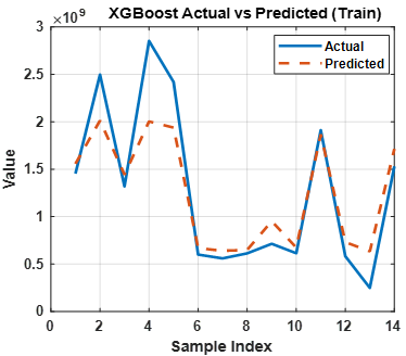
In the training data subset (Figure 12), the fitted curve more or less follows the overall trajectory but has some noticeable smoothing bias. The magnitudes of the upper peaks (indices 1–5) are always smaller than those measured, and the large trough preceding the next spike is flattened, giving values larger than those of the empirical observations. The following ascending (indices around 12–14) is temporally linked, but of smaller amplitude. In the mid-range intervals, the model-observation correspondence is significantly enhanced, signaling greater fidelity in periods of more gradual variation in the signal.
Figure 12. Actual vs. predicted (training data)
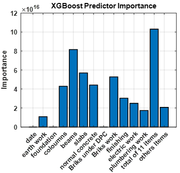
The importance profile is highly skewed (Figure 13). Other items attain the largest score, followed by beams as a clear second tier. A mid-level group comprises slabs, brickwork, normal concrete, and finishing, each contributing appreciably. Lower contributions appear for electric work, plumbing work, and a total of 11 items. Near-negligible influence is observed for date, columns, foundation, and bricks under DPC. In general, the variance explanation is concentrated in some limited set of predictors with diminishing impact in the remaining categories.
Figure 13. Extreme Gradient Boosting (XGBoost) predictor importance
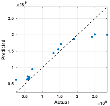
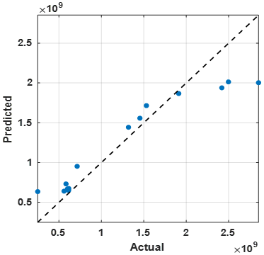
Both parity plots show moderate agreement with the identity line (Figures 14–15), with all measures showing consistent agreement: R2 = 0.851, RMSE ≈ 3.12 × 10⁸, and Train showing R2 = 0.843, RMSE ≈ 3.26 × 10⁸ (values on the target scale). A consistent pattern is observed within the subsets, with observations at low actual values (typically in the range of 0.4–0.7) above the diagonal, a pattern consistent with overprediction, and high-value cases (in the range of 2.2 and above) below the diagonal, a pattern consistent with underprediction. Mid-range points (approximately 1.3–1.9) are close to the diagonal with little dispersion. The absence of significant curvature or isolated outliers and the similarity between the two panels imply rather stable calibration characteristics, whereby the predictions follow the direction closely but show a compression of amplitude at the extreme.
Figure 14. Extreme Gradient Boosting (XGBoost) parity (all set)
Figure 15. Extreme Gradient Boosting (XGBoost) parity (training)
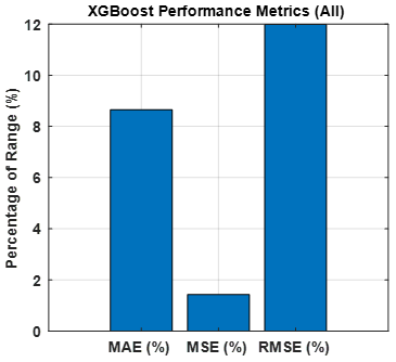
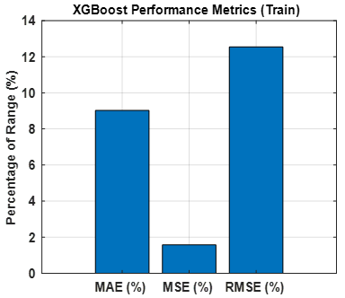
Both panels’ report errors as percentages of the target range and provide a coherent profile (Figures 16–17). The MAE falls within the midrange (around 8–9%), whereas the RMSE is significantly higher (around 12–12.5%), suggesting there are large deviations in comparison to MAE. The market MSE bar is much smaller (around 1–2%) because it is normalized by the squared range and therefore has a compressed scale. Due to the regularization approach and limitation of tree depth, the XGBoost model showed systematic compression. Even though this setting ensures model stability and minimizes overfitting, the model's ability may be restricted to reproduce extreme cost cases. Consequently, this results in overestimating and underestimating for low-cost and high-cost components, respectively. This performance reveals that the XGBoost model works more smoothly for stable trend problems than for holding sharp cost peaks in the case of small datasets.
Figure 16. Extreme Gradient Boosting (XGBoost) performance metrics (all set)
Figure 17. Extreme Gradient Boosting (XGBoost) performance metrics (training)
The similarity of the All and Train charts implies a similar error structure across subsets with just a few differences in magnitude and no indication of disproportionate dispersion clustered around a certain value band.
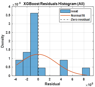
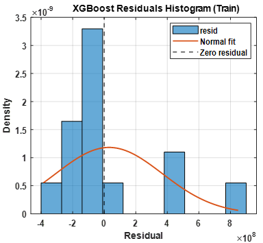
Both density histograms show mass concentration to the left of the zero-error line and a mode at around – (1–2) × 108, thus proving systematic overprediction (Figures 18–19). A pronounced right-hand tail out to about (+8 × 10⁸) is indicative of rare, large underprediction events at high values. The distributions are unimodal but strongly non-Gaussian; the overlaid normal distribution underestimates the tail heaviness. The training subset exhibits similar asymmetry with a slightly narrower spread, indicating the apparent skewness and amplitude to be the features of the fitted mapping rather than effects of the sampling variance. Overall dispersion is on the order of (–4 × 10⁸) to (+8 × 10⁸), with the right skew dominated by the extended right-hand tail.
Figure 18. Extreme Gradient Boosting (XGBoost) residuals histogram (all set)
Figure 19. Extreme Gradient Boosting (XGBoost) residuals histogram (training)
3.3 Adaptive Boosting model
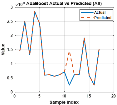
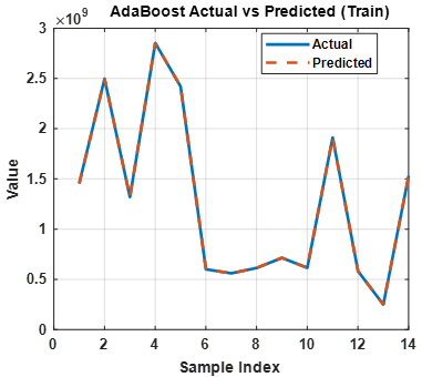
Across both panels, the predicted series mirrors the salient dynamics of the actual sequence, reproducing early high peaks, the sustained mid-range plateau, and the late surge. In the All view (Figure 20), agreement is broadly close with preserved phase alignment; a localized divergence appears around indices (~10–12), where the prediction forms an elevated arch while the actual series remains comparatively flat. Outside this interval, deviations are small and largely symmetric. In the Training view (Figure 21), the two curves are nearly indistinguishable across the entire span, matching both timing and amplitude of oscillations. The juxtaposition indicates highly faithful in-sample reconstruction and generally coherent tracking on the aggregate set, with discrepancies confined to a narrow mid-sequence segment.
Figure 20. Adaptive Boosting (AdaBoost) actual vs predicted (all set)
Figure 21. Adaptive Boosting (AdaBoost) actual vs predicted (training)
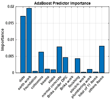
The importance profile is distinctly left-skewed (Figure 22), with date and earth work exhibiting the largest contributions to the fitted mapping. A secondary tier is formed by other items, slabs, brickwork, and normal concrete, which together account for a meaningful share of explanatory power. Moderate but smaller weights appear for finishing. Minimal influence is assigned to columns, beams, bricks under DPC, electric work, plumbing work, and a total of 11 items. Overall, variance attribution is concentrated in a limited subset of predictors, with a clear drop-off across the remaining features.
Figure 22. Adaptive Boosting (AdaBoost) predictor importance
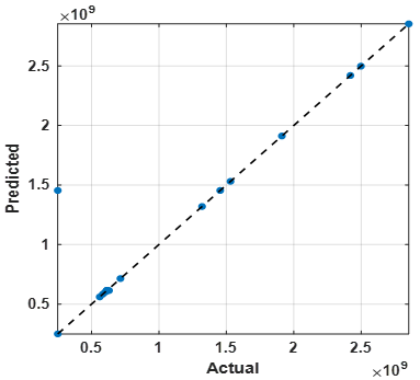
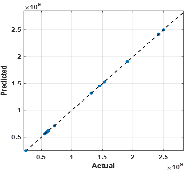
Both parity plots show predictions tightly aligned with the identity line. On all data (Figure 23), points across the full scale $\left(\times 10^9\right)$ cluster near $y=x$, with $\left(\mathrm{R}^2=0.869\right)$ and RMSE $\approx 2.92 \times 108$; alignment is strongest at low $(\approx 0.45-$ $0.7)$ and high $(\approx 2.3-2.7)$ magnitudes, with no visible curvature. On the Training set (Figure 24), the markers lie exactly on the diagonal, yielding $\mathrm{R}^2=1.000 \mathrm{~h}$ and $\mathrm{RMSE}=0$. The visual patterns across both panels are consistent, showing near-identity mapping of predicted to observed values with minimal dispersion and no systematic offset.
Figure 23. Actual vs. predicted (all set)
Figure 24. Actual vs. predicted (training)
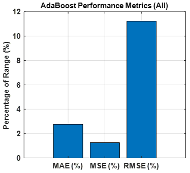
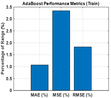
The All panel shows MAE at roughly 2.7% of the target range, MSE near 1.2% (normalized by the squared range), and a markedly higher RMSE of about 11%. This indicates the presence of infrequent but large deviations that increase the RMSE and MSE values relative to MAE (Figures 25-26). In comparison, the training panel shows a compact profile, with MAE of approximately 1%, RMSE of approximately 1.6%, and MSE of approximately 2.3%, which is consistent with a tight in-sample fit. The disparity between panels is similar to previous results on parity and overlay: out-of-sample errors are concentrated in a small number of cases, while in-sample errors are small and equally distributed throughout the response range.
Figure 25. Adaptive Boosting (AdaBoost) performance metrics (all set)
Figure 26. Adaptive Boosting (AdaBoost) performance metrics (training)
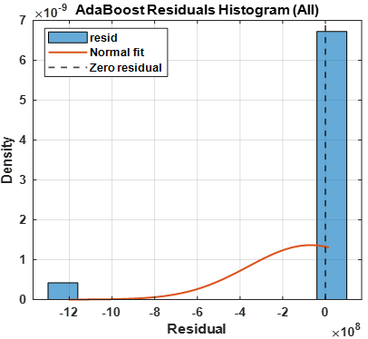
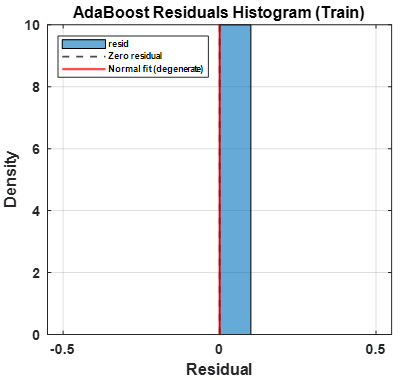
The All histogram concentrates almost all mass at residuals near zero, with a conspicuous single left-tail bar around ( $-1.2 \times 10^9$, units $\times 10^8$ ), producing a strongly skewed, non-Gaussian shape; the normal overlay fails to capture this tail (Figures 27-28). The Training histogram collapses to a vertical spike at zero, yielding a degenerate distribution consistent with perfect in-sample fit. Taken together, the panels indicate predominantly near-zero errors punctuated by a rare, large negative residual out of sample, while training residuals exhibit virtually no dispersion and align exactly with the zero-error line.
Figure 27. Adaptive Boosting (AdaBoost) residuals histogram (all set)
Figure 28. Adaptive Boosting (AdaBoost) residuals histogram (training)
As shown in Table 2, the residual percentile ranges (5th – 95th) were defined to support uncertainty interpretation. They serve as an empirical error band. GBRT model showed the balanced and narrowest residual interval. XGBoost exhibited asymmetric uncertainty due to its tendency to underestimate high-cost components. Conversely, AdaBoost showed a low median error with significant sensitivity to rare extreme residuals.
Table 2. Residual uncertainty summary for all models
|
Model |
GBRT |
XGBoost |
AdaBoost |
|
Mean residual |
2.79 × 10⁷ |
–1.8 × 10⁸ |
–3.97 × 10⁸ |
|
Standard deviation of residuals |
1.35 × 10⁸ |
1.79 × 10⁸ |
6.99 × 10⁸ |
|
5th percentile |
–1.26 × 10⁸ |
–3.86 × 10⁸ |
–1.20 ×10⁹ |
|
95th percentile |
1.23 × 10⁸ |
–5.37 × 10⁷ |
1.59 × 10⁷ |
|
Interpretation |
Residuals are centrally distributed around zero with moderate variance; this indicates stable predictive performance with a marginal tendency toward underprediction. |
Predominantly negative residuals that confirm a systematic overprediction and reflect biased prediction performance throughout most of the dataset. |
The residuals exhibit a strong negative bias with significant dispersion; this reflects a substantial overprediction tendency and poor generalization stability. |
Within the scope and size of the current dataset, the GBRT model showed the most considerable performance among the other adopted models. With low scaled error, GBRT achieved high precision for actual costs. XGBoost model provided stable predictions but overestimated low values and underestimated high values of cost cases. Furthermore, the AdaBoost model revealed a clear generalization gap even with perfect training performance; this reflects an overfitting risk. These conclusions support the GBRT model as a perfect one for this limited dataset. More validation with larger and external databases will be required to generalize the application of these models.
Feature attribution reveals a consistent signal: construction cost drivers dominate. In GBRT and XGBoost, beams and other items carry the greatest importance, with slabs and normal concrete secondary; AdaBoost highlights date and earthwork, then converges on other items, slabs, brickwork, and normal concrete.
The results of feature importance identify structural components, particularly beams, as a primary strong predictor of total construction cost. Moreover, these results reflect a model-based association and do not strictly imply that these features cause the cost variations. These findings prove that boosting-based models effectively provide a trusted tool for early-stage estimation of construction cost, especially when the purpose is to handle the nonlinear relations among the principal cost components. It provides useful evidence that structural components and aggregated items played critical roles for project managers during early cost planning and development of the Bill of Quantities.
[1] Bettini, C.R., Longo, O.C., Alcoforado, L.F., Maia, A.C.G. (2016). Method for estimating of construction cost of a building based on previous experiences. Open Journal of Civil Engineering, 6(5): 749-763. https://doi.org/10.4236/ojce.2016.65060
[2] Yalçın, G., Bayram, S., Çıtakoğlu, H. (2024). Evaluation of earned value management-based cost estimation via machine learning. Buildings, 14(12): 3772. https://doi.org/10.3390/buildings14123772
[3] Sharma, V., Zaki, M., Jha, K.N., Krishnan, N.M.A. (2022). Machine learning-aided cost prediction and optimization in construction operations. Engineering, Construction and Architectural Management, 29(3): 1241-1257. https://doi.org/10.1108/ECAM-10-2020-0778
[4] Pham, T.Q.D., Le-Hong, T., Tran, X.V. (2023). Efficient estimation and optimization of building costs using machine learning. International Journal of Construction Management, 23(5): 909-921. https://doi.org/10.1080/15623599.2021.1943630
[5] Kothapalli, S. (2025). Deep neural networks for predictive construction cost modeling: A multi-algorithm comparative framework with real-time implementation validation. International Journal of Multidisciplinary Research and Growth Evaluation, 6(2): 1898-1905. https://doi.org/10.54660/.ijmrge.2025.6.2.1898-1905
[6] Almahameed, B.A., Bisharah, M. (2024). Applying machine learning and particle swarm optimization for predictive modeling and cost optimization in construction project management. Asian Journal of Civil Engineering, 25: 1281-1294. https://doi.org/10.1007/s42107-023-00843-7
[7] Li, J.L., Wang, Z.T., Zhang, S., et al. (2022). Machine-learning-based capacity prediction and construction parameter optimization for energy storage salt caverns. Energy, 254: 124238. https://doi.org/10.1016/j.energy.2022.124238
[8] Antoniou, F., Konstantinidis, K. (2025). Client-oriented highway construction cost estimation models using machine learning. Applied Sciences, 15(18): 10237. https://doi.org/10.3390/app151810237
[9] Chen, G.L., Zheng, S.M., He, X.R., Liang, X., Liao, X.H. (2025). Machine learning-based cost estimation models for office buildings. Buildings, 15(11): 1802. https://doi.org/10.3390/buildings15111802
[10] Uysal, F., Sonmez, R. (2023). Bootstrap aggregated case-based reasoning method for conceptual cost estimation. Buildings, 13(3): 651. https://doi.org/10.3390/buildings13030651
[11] Jadhav, J.M., Shinde, J.M. (2025). Artificial intelligence and machine learning applications in construction cost forecasting: Model evaluation and web-based deployment. Journal of Xidian University, 19(9): 359-366. https://doi.org/10.5281/zenodo.17129583
[12] Wang, R., Salleh, H., Lyu, J., Abdul-Samad, Z., Radzuan, N.F.M., Wen, K.C. (2025). Application and prospect of machine learning techniques in cost estimation of building projects. Engineering, Construction and Architectural Management, 32(12): 8445-8471. https://doi.org/10.1108/ECAM-05-2024-0595
[13] Park, U., Kang, Y., Lee, H., Yun, S. (2022). A stacking heterogeneous ensemble learning method for the prediction of building construction project costs. Applied Sciences, 12(19): 9729. https://doi.org/10.3390/app12199729
[14] Ugur, L.O., Kanit, R., Erdal, H., et al. (2019). Enhanced predictive models for construction costs: A case study of Turkish mass housing sector. Computational Economics, 53: 1403-1419. https://doi.org/10.1007/S10614-018-9814-9
[15] Tijanić Štrok, K. (2026). Potential of different machine learning methods in cost estimation of high-rise construction in Croatia. Information, 17(1): 91. https://doi.org/10.3390/info17010091
[16] Alshboul, O., Shehadeh, A., Almasabha, G., Almuflih, A.S. (2022). Extreme gradient boosting-based machine learning approach for green building cost prediction. Sustainability, 14(11): 6651. https://doi.org/10.3390/su14116651
[17] Ulfa, Z.M., Prasetyo, A.D. (2020). Financial feasibility study of the construction of new high school building (Case study of XYZ Foundation). European Journal of Business and Management Research, 5(4): 1-6. https://doi.org/10.24018/ejbmr.2020.5.4.467
[18] Elsayed, M., Khalil, A., Mohammed, S., Attia, T. (2023). Developing a model for enhancing cost monitoring and control in the construction firms. International Journal of Advanced Engineering and Business Sciences, 4(2): 110-143. https://doi.org/10.21608/ijaebs.2022.165191.1053
[19] Velumani, P., Nampoothiri, N.V.N. (2019). Analysis of construction cost prediction studies—Global perspective. International Review of Applied Sciences and Engineering, 10(3): 275-281. https://doi.org/10.1556/1848.2019.0032
[20] Zhang, M., Tang, G. (2023). Project construction cost control under the mode of bill of quantities. Frontiers in Science and Engineering, 3(4): 7-11. https://doi.org/10.54691/fse.v3i4.4750