Mohammad A. N. Al-Azawi* | Ali Hamad Al-Badi | Bacem Mbarek
© 2026 The authors. This article is published by IIETA and is licensed under the CC BY 4.0 license (http://creativecommons.org/licenses/by/4.0/).
OPEN ACCESS
Brain abnormality detection from magnetic resonance imaging (MRI) remains challenging due to the large variation in brain anatomy among individuals. Conventional approaches often rely on direct comparison between different subjects, which may reduce diagnostic reliability because of anatomical differences. This study proposes a symmetry-based framework for brain abnormality detection by exploiting the inherent bilateral structure of the human brain. Eighteen first-order statistical (FOS) features were extracted from the differences between corresponding regions of the left and right brain hemispheres to quantify structural asymmetry. Feature relevance was evaluated using correlation analysis, mutual information (MI), and machine-learning-based assessment methods to identify the most discriminative feature subset. The selected features were subsequently classified using four machine learning algorithms, including Random Forest (RF), Support Vector Machine (SVM), Logistic Regression, and Bernoulli classifiers. The proposed framework was evaluated on a dataset consisting of 3,053 axial MRI images, including 1,445 abnormal cases and 1,608 normal cases. Among the evaluated classifiers, the RF model achieved the best performance, with an accuracy of 95.85%, precision of 96%, recall of 96%, and F1-score of 96%. The results demonstrate that bilateral symmetry analysis combined with statistical feature evaluation provides an interpretable and computationally efficient approach for MRI-based brain abnormality classification.
brain magnetic resonance imaging, features, bilateral symmetry, first-order statistical features, feature selection, machine learning, computer-aided diagnosis
Computer-aided diagnostic (CAD) systems are systems developed to help radiologists and specialists interpret medical images using specialised computer systems to improve diagnostic accuracy, save effort and time, and minimise errors. Such systems use various computer technologies, such as image processing and artificial intelligence, to perform their functions. Medical image analysis and processing techniques are important parts of CAD systems as they are used to analyse medical images such as magnetic resonance imaging (MRI) and computed tomography (CT) images and produce results that can help specialists make appropriate decisions. In addition, artificial intelligence techniques are widely used in these systems due to their speed and accuracy in obtaining accurate results.
The identification of brain anomalies using MRI has gained considerable attention over the past few decades due to advances in computer technologies, particularly in digital image processing and artificial intelligence techniques. These advancements have encouraged researchers to explore, develop, and publish innovative approaches in this field. Most MRI analysis approaches involve five stages of processing: (i) pre-processing, (ii) feature extraction, (iii) feature selection, (iv) classification, and (v) segmentation. In this research, our focus is placed on the second and third stages, namely, feature extraction and feature selection.
The considerable variation in brain shape among individuals represents a major challenge in the computer-based diagnosis process. Therefore, the process of diagnosing a person’s brain based solely on others’ brain images may not be sufficiently reliable.
This study is a continuation of our previous work in this field, where we demonstrated the potential of using the symmetry between the two brain hemispheres for accurate abnormality detection. Brain tumours can alter the shape and structure of one hemisphere, resulting in a disruption of the natural bilateral symmetry of the brain [1, 2]. In this study, we investigated 18 first-order statistical (FOS) features and evaluated their significance in enhancing brain abnormality identification accuracy using various feature evaluation measures, including mutual information (MI), correlation analysis, and machine learning-based evaluation methods.
Unlike conventional MRI-based brain abnormality detection methods, the proposed framework exploits the inherent bilateral symmetry of the brain to quantify structural abnormalities. Furthermore, rather than employing all extracted features, this study systematically evaluates the discriminative capability of eighteen FOS features using correlation analysis, MI, and machine learning-based evaluation to identify the most informative subset for classification. This combination provides a simple, interpretable, and computationally efficient framework for brain abnormality detection. The proposed framework contributes to intelligent information processing in medical imaging by transforming brain MRI data into discriminative symmetry-based representations for automated brain abnormality detection. By integrating statistical feature extraction, feature evaluation, and machine learning, the framework provides an efficient information processing pipeline that supports CAD and enhances the capability of medical information systems to analyse brain MRI data.
The remainder of this paper is structured as follows: Section 2 presents the necessary theoretical background and reviews state-of-the-art studies. The proposed approach is presented in Section 3. In Section 4, a thorough discussion and evaluation of the obtained results are presented. Finally, conclusions are presented in Section 5.
2.1 Magnetic resonance imaging analysis
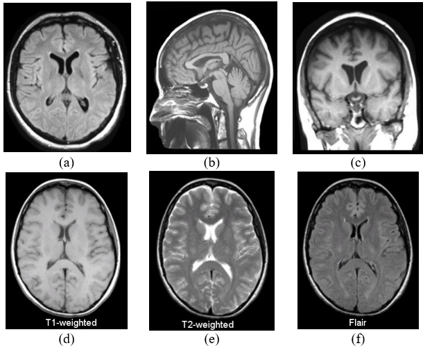
MRI is widely used in neurology, neurosurgery, and many other medical fields because it offers excellent visualisation of the brain. MRI can visualise the brain in three planes: axial, sagittal, and coronal, as shown in the samples in Figures 1(a)–(c). Furthermore, three sequences are commonly used in MRI, namely T1-weighted (T1W), T2-weighted (T2W), and FlAIR. The difference between the various types of sequences results from the selection of Time to Echo (TE) and Repetition Time (TR), where T1W images are produced using short TE and short TR, while T2W images are generated using longer TE and TR times. The Flair sequence is similar to T2W but with very long TE and TR values. The three forms of sequences are shown in Figures 1(e)–(g) [3].
2.2 Brain abnormality identification techniques
Brain abnormality identification is a challenging task because of the structural complexity of brain tissue. Usually, this can be done in one of three ways, depending on the level of human intervention: manual, semi-automatic, and fully automatic [4, 5]. In the first method, the entire process is performed by the radiologist, whereas in the second method, the specialist interacts with the automatic segmentation system by specifying and initialising some parameters, providing feedback on the system output, and finally evaluating the results. Finally, in fully automatic systems, the machine performs all the operations without user intervention.
Brain tumour identification has been the focus of many studies over the past few decades. Due to the availability of resources and the large amount of published work, many reviews have been published that list the methods and techniques used. The reviews focused primarily on two approaches: non-AI-based approaches that do not utilise AI algorithms, such as thresholding, image segmentation, and clustering [6] and artificial intelligence-based approaches that use AI algorithms such as machine learning, which learns discriminative patterns from MRI-derived features for automated classification [7]; transformer-based models, which employ self-attention mechanisms to capture long-range spatial dependencies in brain images [8]; transfer learning, which adapts knowledge learned from large pre-trained models to improve performance on limited MRI datasets [9]; hybrid AI models, which combine multiple AI techniques to exploit their complementary strengths [10]; and deep learning, which automatically learns hierarchical feature representations directly from MRI images for accurate detection and classification [11, 12].
Despite the considerable progress achieved by both conventional image processing and AI-based techniques, there remains a need for efficient and interpretable methods that maintain high classification performance while reducing computational complexity.
Motivated by this need, the proposed framework utilises bilateral brain symmetry and systematic feature evaluation to develop an effective brain abnormality identification approach.
Figure 1. Brain magnetic resonance imaging (MRI) shows the three planes and the three sequences: (a) axial plane, (b) sagittal plane, (c) coronal plane, (d) T1-weighted (T1W) sequence, (e) T2-weighted (T2W) sequence, and (f) Flair sequence [5]
2.3 Feature extraction (first-order statistics)
FOS features are derived from the histogram, which is a well-known representation of an image and is used to describe the probability density function of the pixel intensities in the image. The histogram consists of bins representing the grey levels and the probability of occurrence of each grey level. The histogram itself cannot be used as a feature; however, a set of statistical features can be extracted from it, known as FOS. The most widely used features are as follows.
1. Central tendency features, which include the mean (F1), median (F2), and mode (F3), can be calculated using Eqs. (1)–(3), respectively.
$\begin{gathered}M=\sum_{x=0}^{N-1} h(x), p(x)=\frac{h(x)}{M} \\ F 1=\sum_{x=0}^{N-1} x \cdot p(x)\end{gathered}$ (1)
$\begin{gathered}h s=Sort(h), n=\frac{N}{2} \\ F 2=h s(n)\end{gathered}$ (2)
$\begin{aligned} n & =Max(\operatorname{Count}(p(x))) \\ F 3 & =p(x) correspondingn\end{aligned}$ (3)
where, $M$ is the number of pixels in the image, $N$ is the number of grey levels (bins), $h(x)$ is the number of pixels which have $x$ value, $p(x)$ is the probability of occurrence of the grey level $x$, and hs is the sorted histogram.
2. Dispersion is another important measure that indicates the extent to which numerical data are likely to vary around an average value. Variance, standard deviation, and coefficient of variation are the most commonly used measures to describe dispersion. These measures describe the spread of the grey levels over the bins and the extent to which each grey level is from the mean. The variance (F4), standard deviation (F5), and coefficient of variation (F6) are calculated as given in Eqs. (4)–(6), respectively.
$F 4=\sum_{x=0}^{N-1}(x-F 1)^2 \cdot p(x)$ (4)
$F 5=\sqrt{F 4}$ (5)
$F 6=\frac{F 5}{F 1}$ (6)
3. Skewness (F7) and kurtosis (F8): The skewness measure describes the distortion that deviates the histogram from the symmetrical normal distribution curve. On the other hand, kurtosis measures the presence of extreme values in the tails of the distribution. Histograms with significant kurtosis show tail data that exceeds that of the normal distribution and vice versa. The skewness (F7) and kurtosis (F8) can be calculated using Eqs. (7) and (8), respectively.
$F 7=\left(\frac{1}{F 5^3}\right) \sum_{x=0}^{N-1}(x-F 1)^3 \cdot p(x)$ (7)
$F 8=\left(\frac{1}{F 5^4}\right) \sum_{x=0}^{N-1}(x-F 1)^4 \cdot p(x)$ (8)
4. Energy (F9) and entropy (F10): These measures are widely used to describe the randomness and information content of a histogram. They can be calculated using the formulas given in Eqs. (9) and (10), respectively.
$F 9=\sum_{x=0}^{N-1}(p(x))^2$ (9)
$F 10=-\sum_{x=0}^{N-1} p(x) \log _2 p(x)$ (10)
5. Ranges and percentiles: The range (F13) is the difference between the maximum (F12) and minimum (F11) values of the histogram, where the maximum and minimum values are the maximum and minimum heights of the histogram. The minimum, maximum, and range can be calculated using Eqs. (11)–(13), respectively:
$F 11=\min _x h(x)$ (11)
$F 12=\max _x h(x)$ (12)
$F 13=F 12-F 11$ (13)
6. The Kth percentile is the percentage of values below a specific K in the histogram. In this work, we consider the 10th, 25th, 75th, and 90th percentiles, which are denoted as (F14, F15, F16, F17), respectively. The 50th percentile was not considered because it represents the median (F2). Finally, the histogram width (F18) is the difference between the 90th and 10th percentiles and is calculated using Eq. (14).
$F 18=F 17-F 13$ (14)
Table 1 summarises the features discussed above.
Table 1. First-order statistical (FOS) feature summary
|
Feature |
Feature Name |
Eq. |
Feature |
Feature Name |
Eq. |
Feature |
Feature Name |
Eq. |
|
F1 |
Mean |
(1) |
F7 |
Skewness |
(7) |
F13 |
Range |
(13) |
|
F2 |
Median |
(2) |
F8 |
Kurtosis |
(8) |
F14 |
10th Percentiles |
|
|
F3 |
Mode |
(3) |
F9 |
Energy |
(9) |
F15 |
25th Percentiles |
|
|
F4 |
Variance |
(4) |
F10 |
Entropy |
(10) |
F16 |
75th Percentiles |
|
|
F5 |
Standard deviation |
(5) |
F11 |
Minimal Value |
(11) |
F17 |
90th Percentiles |
|
|
F6 |
Coefficient of variation |
(6) |
F12 |
Maximal Value |
(12) |
F18 |
Width of Histogram |
(14) |
2.4 Feature evaluation
2.4.1 Correlation factors
The correlation coefficient is a descriptive statistical number that describes the strength and direction of the relationship between variables. It takes values between –1 and 1, where the magnitude indicates the strength of the relationship and the sign reflects its direction. Pearson, Kendall, and Spearman coefficients are the most commonly used correlation factors. The following discussion provides a simple explanation of the three types of correlation factors.
1. The Pearson correlation factor assumes that the relationship between the two variables is linear, both variables are normally distributed, and the data are equally distributed about the regression line. Pearson correlation factor can be calculated using Eq. (15).
$C_p=\frac{\left(\left(n \sum_{i=0}^{n-1} x_i y_i\right)-\left(\sum_{i=0}^{n-1} x_i \sum_{i=0}^{n-1} y_i\right)\right)}{\sqrt{n \sum_{i=0}^{n-1} x_i^2-\left(\sum_{i=0}^{n-1} x_i\right)^2} \sqrt{n \sum_{i=0}^{n-1} y_i^2-\left(\sum_{i=0}^{n-1} y_i\right)^2}}$ (15)
where, $C_p$ is Pearson correlation factor, $n$ is the number of observations, and $x_i$ and $y_i$ are the $i$-th elements of the two variables $X$ and $Y$.
2. Spearman rank correlation, which is given in Eq. (16), is non-parametric, does not carry any assumptions about the distribution of the data, and is appropriate when the variables are measured on a scale that is at least ordinal.
$C_s=1-\frac{\left(6 \sum_{i=0}^{n-1} d_i^2\right)}{n\left(n^2-1\right)}$ (16)
where, $C_s$ is the Spearman correlation factor, $d_i$ is the difference between the ranks of corresponding variables, and $n$ is the number of observations.
3. Kendall correlation coefficient, which is usually referred to as Kendall’s Tau measure, is non-parametric and is used to measure the relationships between columns of ranked data and takes values between 0 and 1, where zero means no relationship and 1 means a perfect relationship. Kendall’s Tau can be calculated using Eq. (17).
$C_c=\frac{C-D}{C+D}$ (17)
where, $C_c$ is Kendall's Tau coefficient, $C$ is the number of concordant pairs and $D$ is the number of discordant pairs.
2.4.2 Mutual information contents
MI $I(X ; Y)$ can be defined as the amount of information that variable $X$ contains about variable $Y$, where $X$ and $Y$ are two discrete random variables. It indicates the level of shared information between the two random variables. In other words, if the value of $I(X ; Y)$ is large, the variables are more related to each other and vice versa [13]. Based on the previous observation, MI has been utilised to select the best feature in classification problems in many studies [14,15].
The most commonly used measure of information content is the entropy from Shannon’s information theory, which is given in Eq. (18).
$H(X)=-\sum_{i=0}^n P(x \mid i) \log _2 P(x \mid i)$ (18)
where, $X$ is a discrete random variable expressed as $X=\left\{x_0, x_1, \ldots, x_n\right\}$ and $P(x \mid i)$ is the probability of occurrence of the variable $x_i$.
Further, let us define a second discrete random variable $Y=\left\{y_0, y_1, \ldots, y_m\right\}$, then the conditional entropy of the variable $Y$, which measures the amount of uncertainty left in the variable $Y$ after the variable $X$ is introduced is calculated using Eq. (19).
$H(Y \vee X)=-\sum_{x_i \in X} \sum_{y_i \in Y} P\left(y_j, x \mid i\right) \log _2 P\left(y_j \vee x \mid i\right)$ (19)
The joint entropy $H(Y, X)$ of $X$ and $Y$ which is defined as the uncertainty that occurs simultaneously with two variables, is calculated as given in Eq. (20).
$\begin{gathered}H(Y, X)=-\sum_{x_i \in X} \sum_{y_i \in Y} P\left(y_j, x \mid i\right) \log _2 P\left(y_j, x \mid i\right) \\ H(Y, X)=H(X)+H(Y \vee X)\end{gathered}$ (20)
Finally, the MI between variable $Y$ and variable $X$ can be calculated using Eq. (21).
$\begin{gathered}I(Y ; X)=\sum_{x \in X} \sum_{y \in Y} P(y, x) \log _2\left(\frac{P(y, x)}{P(x) P(y)}\right) \\ I(X ; Y)=H(X)+H(Y)-H(X, Y)\end{gathered}$ (21)
2.4.3 Machine learning-based
Machine learning can be used to evaluate features by relating independent variables to dependent variables. This is done by dividing the dataset into two sets, one for training and the other for testing. The first set is used to train the model, whereas the second set is used to evaluate the performance and accuracy of the model. Based on the problem under study, it is categorised as a supervised classification problem where the images need to be classified as either normal or abnormal brain images.
Machine learning can be used to evaluate features or assign importance to a particular feature when it is trained on it and to evaluate its accuracy. Although many different models can be used for this purpose, we have considered only four models, namely, Random Forest Classifier (RFC), Naive Bayes Classifier (NBC), Logistic Regression Classifier (LRC), and Support Vector Machine Classifier (SVMC) because of their accuracy and wide use.
RFC was selected because of its robustness to nonlinear feature relationships and its ability to reduce overfitting through ensemble learning. NBC provides a simple probabilistic baseline, while LRC serves as an interpretable linear classifier for assessing feature separability. SVMC was included because of its strong generalisation capability in binary classification problems. The objective of employing these classifiers is not to compare machine learning algorithms, but to validate the effectiveness and robustness of the proposed symmetry-based feature extraction and feature evaluation framework.
This section presents the proposed framework and consists of two main stages: dataset preparation and the proposed system architecture.
3.1 Dataset and experimental environment
The proposed algorithm was implemented in Python 3.10 using JupyterLab 3.4.4. All experiments were executed on a MacBook equipped with an Apple M2 processor comprising an 8-core CPU, a 10-core GPU, and 8 GB of RAM.
As no single publicly available dataset adequately satisfied the requirements of the proposed algorithm, a dataset was constructed by the authors using images collected from the public datasets reported in the studies [16-19]. The resulting dataset comprises 3,053 axial brain MRI images, including 1,445 images with brain cancer and 1,608 normal brain images [20]. The dataset includes T1W, T2W, and Flair MRI sequences. All images are single-channel greyscale images with 256 grey levels and were standardised to a spatial resolution of 200 × 200 pixels prior to processing. When machine learning algorithms were applied, the dataset was randomly divided into 70% training data and 30% testing data using stratified sampling to preserve the proportions of normal and cancer cases in both subsets.
3.2 Proposed framework
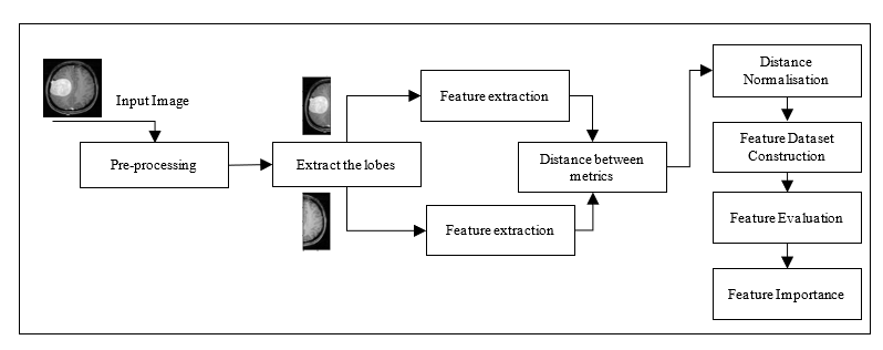
The implementation of the model is illustrated in Figure 2. In this flowchart, the image undergoes preprocessing operations such as image restoration, skull removal, and other pre-processing operations [2]. After the pre-processing stage, the image $J_i$ is divided around the vertical axis into two sub-images which are the left lobe image $L_i$ and the right lobe image $R_i$. No image registration was performed as the images were axial MRI that had already been spatially standardised in their source datasets. Each image was divided along its vertical axis before proceeding with the rest of the processes. Next, the features are extracted from each sub-image $M L_i$ and $M R_i$ and the distances between the opposite features are calculated to obtain the distance vector $\left(d_i=\left\{\delta_{i, 1}, \delta_{i, 2}, \ldots, \delta_{i, n}\right\}\right)$. The distance vector is then normalised to be in the range of $(0,1)$ which produces the normalized distance vector $\left(\dot{d}_l=\left\{\delta_{l, 1}^{\prime}, \delta_{l, 2}^{\prime}, \ldots, \delta_{l, n}^{\prime}\right\}\right)$. Finally, the feature dataset is constructed after adding the class $\left(c_i\right)$ corresponding to each normalised vector $\dot{d}_{\imath}$, which results in the vector $D_C=$ $\left\{\left(\dot{d}_1, c_1\right),\left(\dot{d}_2, c_2\right), \ldots,\left(\dot{d}_N^{\prime}, c_N\right)\right\}$.
The proposed architecture constitutes an intelligent information processing framework that converts raw MRI images into clinically meaningful information through symmetry-based feature extraction, feature evaluation, and machine learning-based classification.
The second part of the algorithm is to study the importance of each feature and its role in identifying the features that have a larger impact on the classification process. Three methods of feature evaluation have been studied, namely: correlation, MI, and machine-learning-based techniques.
When machine learning algorithms were employed, the dataset was randomly divided into two sets: one for training, which consists of 70% of the data, and the other for testing and includes 30% of the images in the dataset. This splitting was performed using stratified sampling to preserve the proportions of normal and abnormal cases in both subsets.
Figure 2. Model implementation
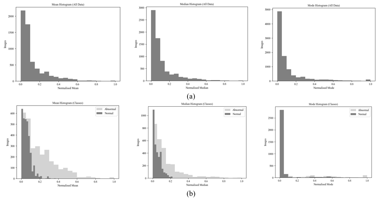
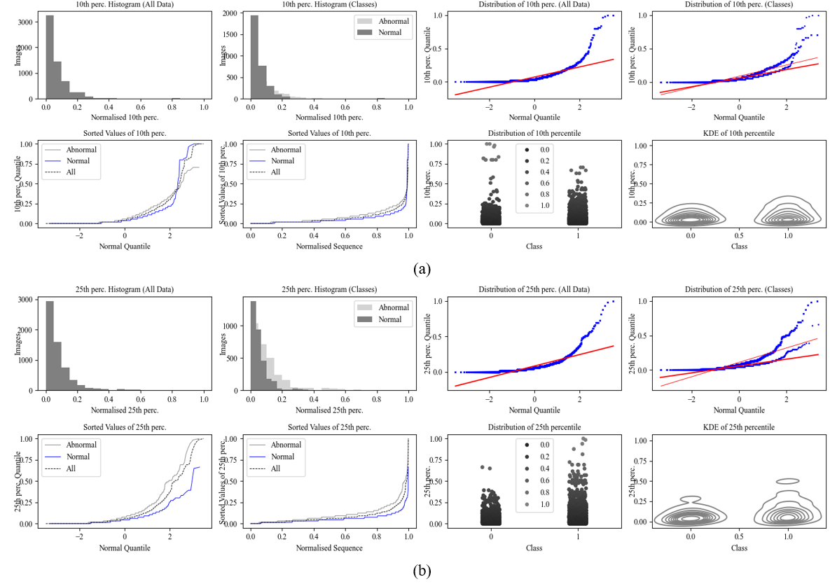
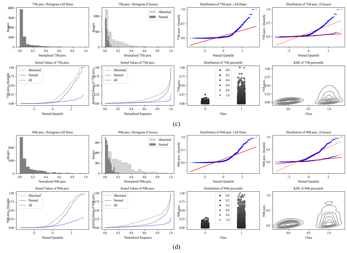
In this section, we discuss the results obtained by applying the proposed method to a standard dataset containing 3053 brain images [20]. In this discussion, several graphs were used to illustrate the results in addition to the listed values. The first graph used is the histogram, which shows the frequency of data items in successive numerical intervals of equal size. In our problem, there are no fixed values for the variables; hence, the interval was divided into 20 bins of equal intervals. Quantile-Quantile plot (Q-Q plot), which is a graphical tool that helps evaluate whether a data set is close to a theoretical distribution such as a normal distribution, is the second graph used to describe the result. The points in the graph are extracted by determining the differences between the dataset and a normal distribution at a specific point. In this illustration, the ideal case is when the data in the dataset is normally distributed, where the relationship represents a straight line; in other words, the more linear the relationship, the fewer the anomalies. In addition to the previous graphs, a strip plot was used in the discussion; the strip plot is a scatter plot that has a single axis and is used to represent the distribution of many individual one-dimensional values. The values are plotted as small filled circles along one axis, with circles with similar values overlapping. Two strip plots, one for each class, were placed side-by-side to compare the distributions of data points between the two classes (normal and abnormal). Finally, the Kernel Distribution Estimation (KDE) plot) was used as well. The KDE plot is a method for representing and visualizing the distribution of the data in a dataset in a manner similar to a histogram. The KDE represents data using a continuous probability density curve in one or more dimensions.
In the following discussion, to save space and avoid unnecessary redundancy, we will discuss the graphs for central tendency only, as the rest of the features follow similar descriptions.
4.1 Central tendency
The central tendency features, which include the mean (F1), median (F2), and mode (F3), were calculated using Eqs. (1)–(3). The histograms of the obtained results for the three features, mean, median, and mode, are given in Figure 3, where Figure 3(a) gives the histograms of the three features for all data and Figure 3(b) displays their histograms according to the classes (Normal and Abnormal). It is clear from the figure that the normalised values of the mean, median, and mode of the abnormal cases are more widely distributed than in the normal cases because the differences between the features in the first class are greater than those in the second class.
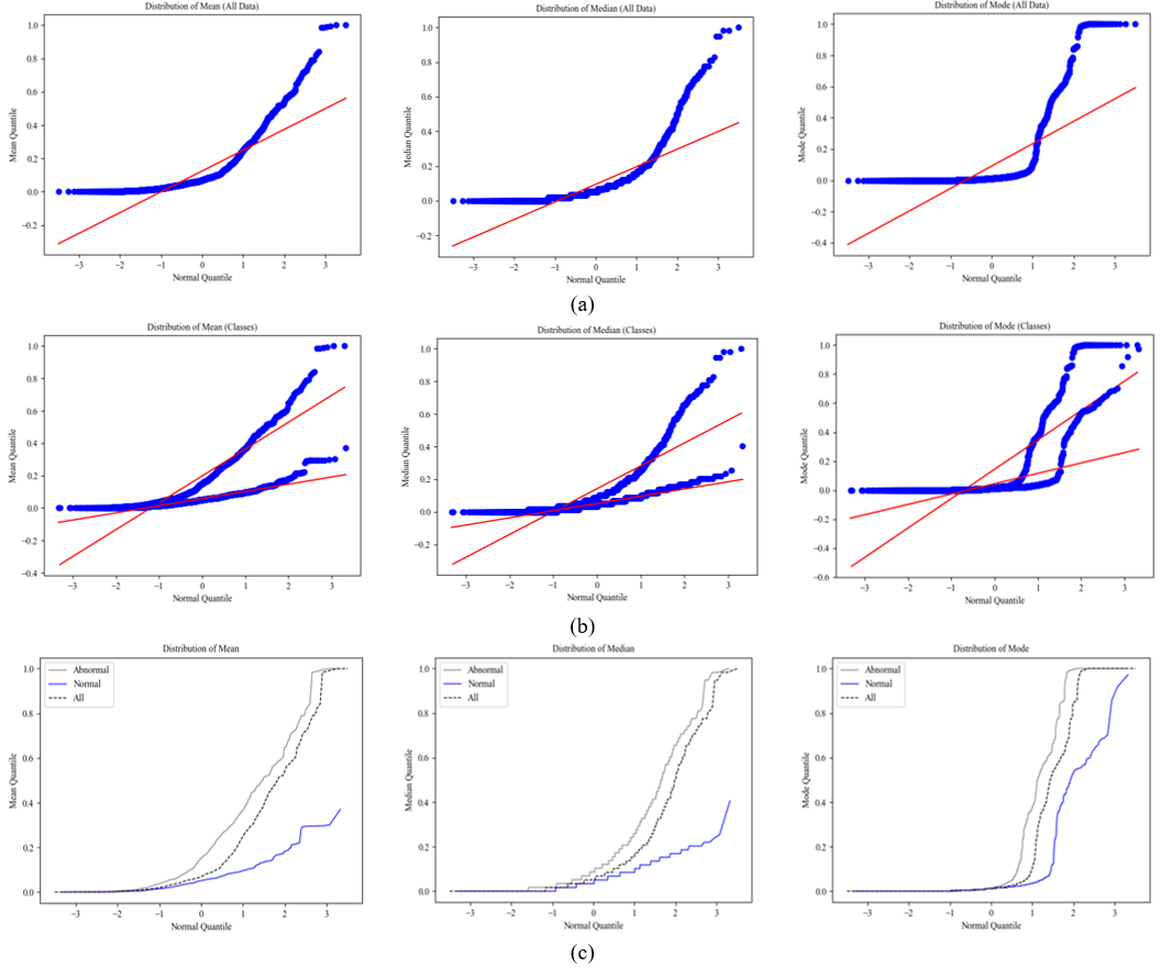
Figure 4 shows the Q-Q plot of the central tendency features. Figure 4(a) shows the Q-Q plot of the entire data in the dataset; Figure 4(b) gives the Q-Q plot of the two classes separately, and Figure 4(c) shows the comparison of the Q-Q plots of the entire dataset, the normal brain data, and the abnormal brain data.
In Figure 4(a), the graph shows that there is a clear difference between the data in the dataset and the normal brain distribution, whereas the best case is with the median. On the other hand, the feature distribution of normal brains is closer to the normal distribution, as there are fewer anomalies compared to the features of abnormal brains, which is evident from the straight-line approximation of the feature curves for both classes as shown in Figure 4(b).
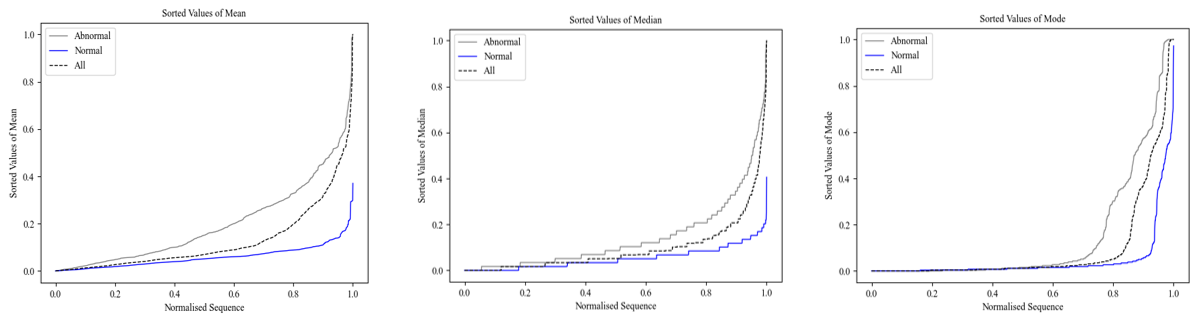
Figure 5 shows the sorted normalised values of the mean, median, and mode for the three cases, which are all data (All), normal brain data (Normal), and abnormal brain data (Abnormal). From this figure, it is obvious that the values of the features of the abnormal brain data are larger than those of the normal brain data, and this indicates that the difference between the features of the two lobes is greater.
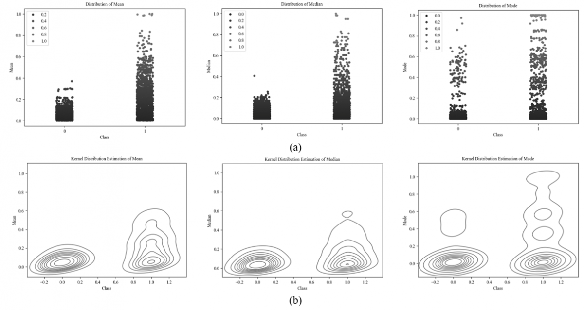
Figure 6 shows the strip plot Figure 6(a) and the KDE Figure 6(b) of the three features. From the figure, it is clear that the distribution of the mean and median of normal brains is in the range of 0 to 0.2, while the mode has some anomalies, and the values may exceed 0.2. On the other hand, the distribution of abnormal brain features is between 0 and 1 and is larger than that of normal brains. The same applies to Figure 6(b), which shows the KDE distribution.
4.2 Dispersion
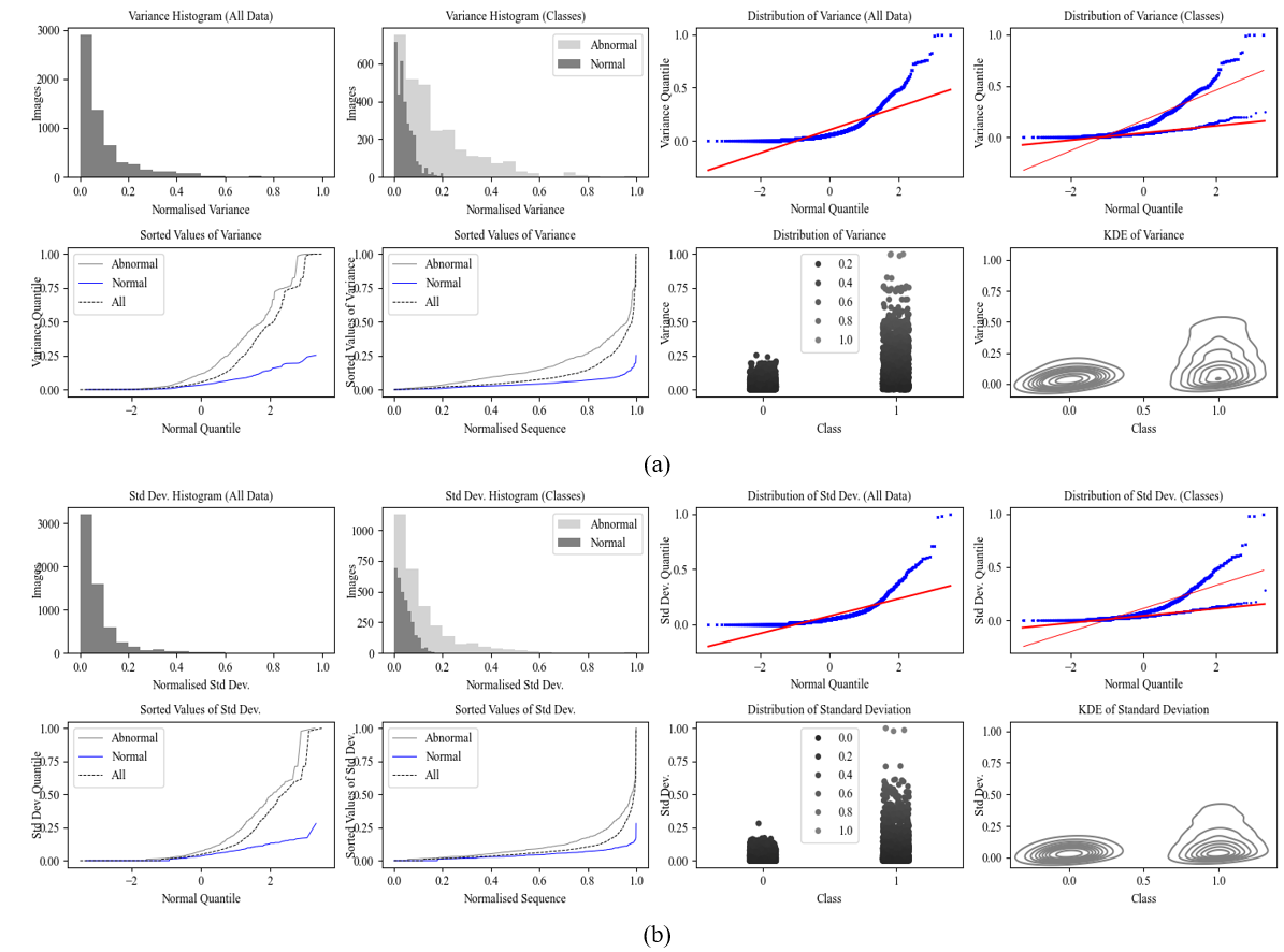
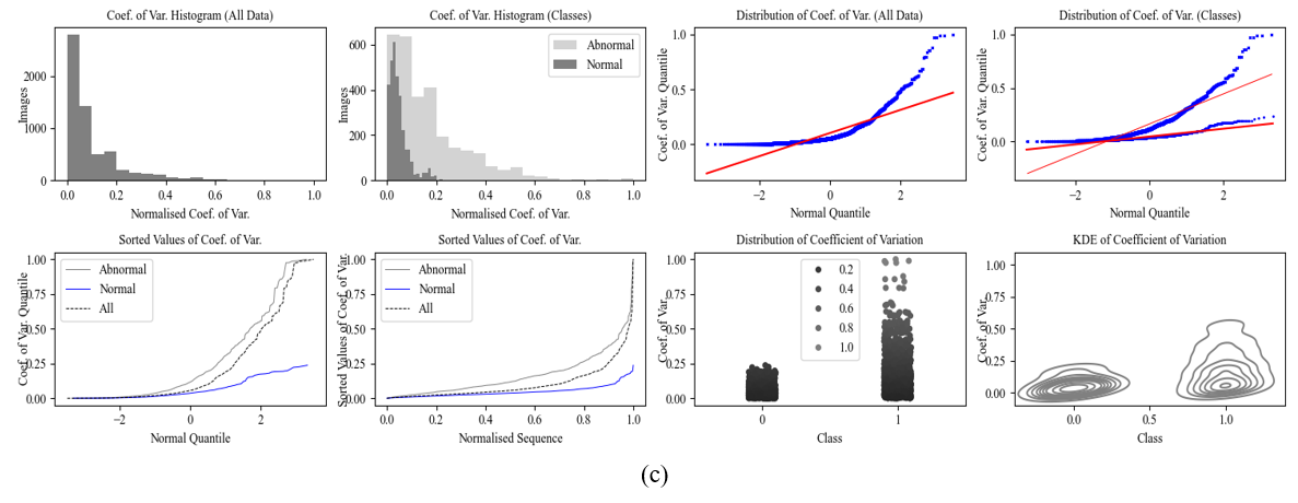
The dispersion features, which include the variance (F4), standard deviation (F5), and coefficient of variation (F6), are calculated using Eqs. (4)–(6), respectively. The graphical representation of these features is given in Figure 7, where Figure 7(a) shows the graphical representation of the variance, Figure 7(b) shows the graphs of the standard deviation, and Figure 7(c) shows the coefficient of variation. The distribution of the data for all features is somewhat similar to that of the central tendency features. However, the main observation here is that the distribution of the normal brain data is close to being normal, while that of the abnormal brain data has dispersion.
Figure 3. Histogram representation of the central tendency features (mean, median, and mode respectively): (a) histograms of all images, (b) histograms according to the classes: normal and abnormal
Figure 4. Probability distribution representation of the central tendency features (mean, median, and mode respectively): (a) probability distribution of all images, (b) probability distribution according to the class, (c) probability distribution representation of all brain images (All), normal brain images (Normal), and abnormal brain images (Abnormal)
Figure 5. The sorted values of the central tendency features (mean, median, and mode respectively) of all brain images (All), normal brain images (Normal), and abnormal brain images (Abnormal)
4.3 Skewness and kurtosis
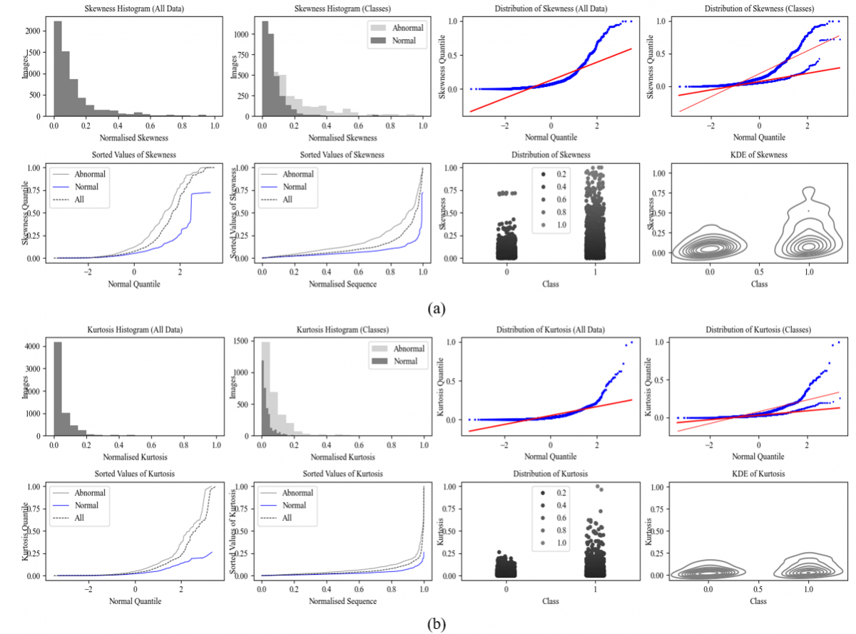
The Skewness (F7) and Kurtosis (F8) can be calculated using Eqs. (7) and (8), respectively. Figure 8 shows these two features, in which Figure 8(a) represents skewness and Figure 8(b) represents kurtosis. From the figure, it is evident that the values of the measurements extracted from the normal brain data are lower than those of the abnormal brain data; however, the distribution of the data follows a normal distribution to a lesser extent than in the previous features.
Figure 6. Results’ distribution of central tendency features (mean, median, and mode respectively): (a) strip plot, (b) Kernel Distribution Estimation (KDE) plot
Figure 7. Graphical representation of the dispersion features: (a) variance, (b) standard deviation, (c) coefficient of variation
Figure 8. Graphical representation of skewness and kurtosis features: (a) skewness and (b) kurtosis
4.4 Energy and entropy
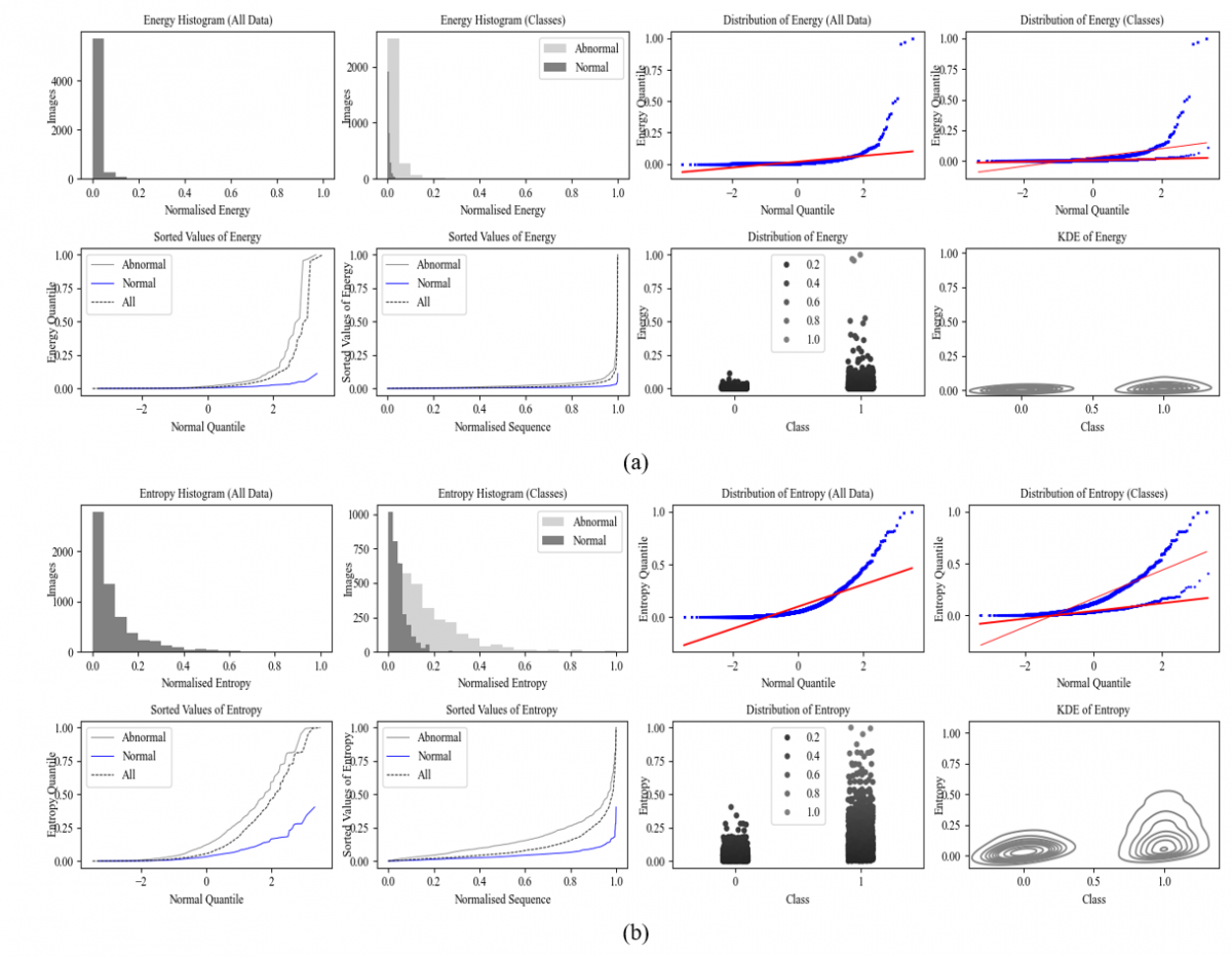
The Energy (F9) and entropy (F10) were evaluated using Eqs. (9) and (10), as shown in Figure 9, where Figure 8(a) shows the energy and Figure 8(b) shows the entropy.
4.5 Ranges
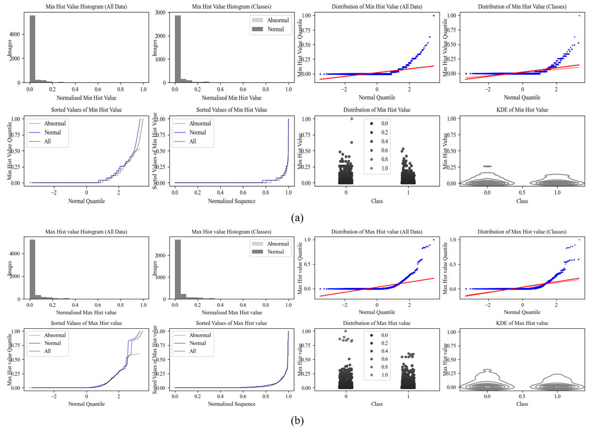
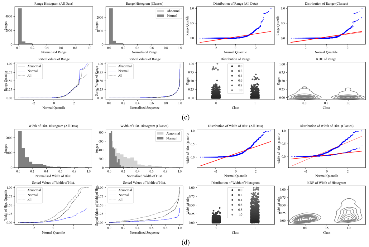
The minimal value (F11), maximal value (F12), range (F13), and width of the histogram (F18) are evaluated using Eqs. (11)–(14), respectively. The visual representations of the aforementioned features are shown in Figure 10, where Figure 10(a) shows the minimal histogram values, Figure 10(b) shows the maximal histogram values, Figure 10(c) is the range of the histogram, and Figure 10(d) is the width of the histogram.
4.6 Percentiles
The last features used are the percentiles, which include the10th, 25th, 75th, and 90th percentiles and are denoted as (F14, F15, F16, and F17). The graphical representation of the percentiles features is shown in Figure 11, where the10th, 25th, 75th, and 90th percentiles are represented by the graphs in Figures 11(a)–(d), respectively.
Figure 9. Graphical representation of energy and entropy features: (a) energy and (b) entropy
Figure 10. Graphical representation of range features: (a) minimal value, (b) maximal value, (c) range, (d) width of the histogram
Figure 11. Graphical representation of percentile features: (a) 10th percentile, (b) 25th percentile, (c) 75th percentile, (d) 90th percentile
4.7 Features evaluation
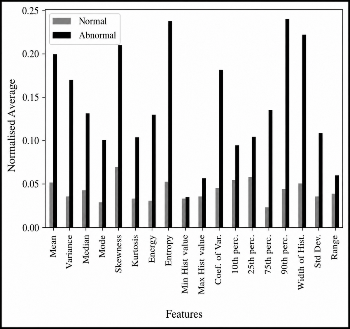
This section presents the analysis and discussion of feature evaluation using the aforementioned methods, namely, correlation, MI content, and machine learning. First, to obtain an overview of the extracted feature values, the average values of the 18 extracted features for normal, abnormal, and overall datasets are presented in Table 2. From the table, it is evident that the values of the features obtained from abnormal brain datasets are generally higher than those obtained from normal brain datasets. From the table, it is evident that the values of the features obtained from the abnormal brain dataset are very much higher than those obtained from the normal brain dataset; this is also explained in Figure 12.
Table 2. Feature averages from the dataset
|
Feature |
Normal |
Abnormal |
All |
|
F1 |
0.052 |
0.199 |
0.126 |
|
F2 |
0.042 |
0.131 |
0.087 |
|
F3 |
0.028 |
0.1 |
0.064 |
|
F4 |
0.035 |
0.17 |
0.103 |
|
F5 |
0.035 |
0.107 |
0.071 |
|
F6 |
0.045 |
0.181 |
0.113 |
|
F7 |
0.069 |
0.22 |
0.145 |
|
F8 |
0.033 |
0.103 |
0.068 |
|
F9 |
0.03 |
0.129 |
0.08 |
|
F10 |
0.052 |
0.237 |
0.145 |
|
F11 |
0.032 |
0.056 |
0.034 |
|
F12 |
0.035 |
0.035 |
0.046 |
|
F13 |
0.039 |
0.059 |
0.049 |
|
F14 |
0.054 |
0.094 |
0.074 |
|
F15 |
0.057 |
0.104 |
0.08 |
|
F16 |
0.022 |
0.134 |
0.079 |
|
F17 |
0.043 |
0.237 |
0.142 |
|
F18 |
0.05 |
0.222 |
0.136 |
Figure 12. Averages of features
4.7.1 Correlation
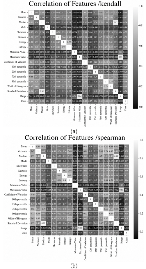
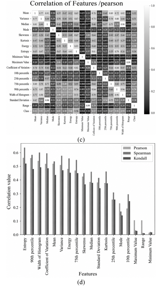
The first evaluation is the correlation, which is used to relate the extracted features to the output class. The three correlation methods, namely Pearson, Kendall, and Spearman correlation coefficients, have been studied and analysed. The correlation values between the extracted features and the class labels using Pearson, Kendall, and Spearman correlation coefficients are summarised in Table 3. The heatmaps of the three types of correlation are presented in Figure 13, where Figure 13(a) shows the heatmap of the Kendall correlation, and Figure 13(b) and Figure 13(c) show the heatmaps of Spearman and Pearson correlations, respectively.
Figure 13. Correlation heatmaps: (a) Kendall, (b) Spearman, (c) Pearson, (d) values of feature correlation with the class
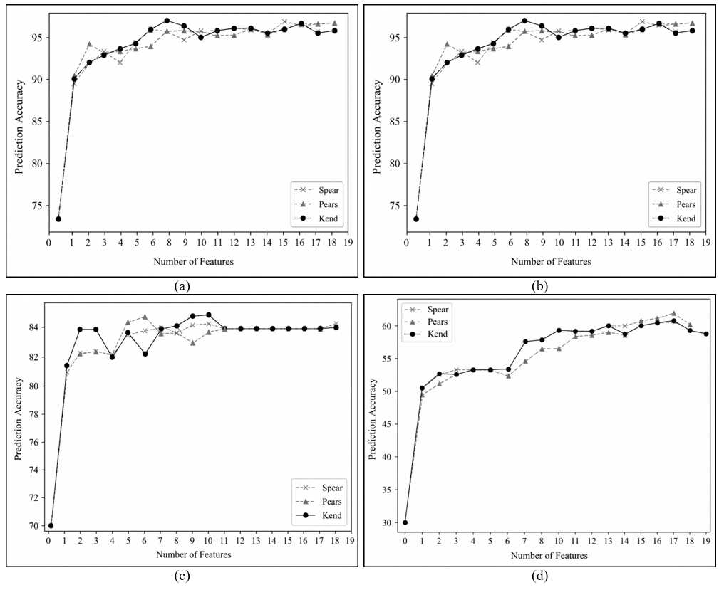
In addition to the statistical correlation analysis, the effect of percentile-based feature selection on the classification performance was investigated using the four machine learning classifiers. Figure 14 illustrates the prediction accuracy obtained using different percentile values for the RFC, Support Vector Machine (SVM), Logistic Regression, and Bernoulli classifiers. The results show that the classification accuracy does not continuously increase with the percentile value; instead, the optimal percentile depends on the employed classifier. This indicates that percentile selection has an important influence on the discriminative capability of the extracted features.
Table 3. Correlation values
|
Feature |
Pearson |
Feature |
Kendall |
Feature |
Spearman |
|
Entropy |
0.585357 |
Entropy |
0.531897 |
Entropy |
0.650814 |
|
90th percentile |
0.579747 |
Coefficient of variation |
0.52079 |
Coefficient of variation |
0.637223 |
|
Width of histogram |
0.555244 |
Width of histogram |
0.508222 |
Width of histogram |
0.618127 |
|
Coefficient of variation |
0.547017 |
90th percentile |
0.495832 |
90th percentile |
0.602158 |
|
Mean |
0.531279 |
Variance |
0.474194 |
Variance |
0.580213 |
|
Energy |
0.522218 |
Mean |
0.459235 |
Mean |
0.561907 |
|
Variance |
0.51684 |
Energy |
0.453498 |
Energy |
0.554886 |
|
75th percentile |
0.478632 |
75th percentile |
0.450132 |
75th percentile |
0.543297 |
|
Skewness |
0.45314 |
Kurtosis |
0.388448 |
Kurtosis |
0.475293 |
|
Kurtosis |
0.40837 |
Skewness |
0.382132 |
Skewness |
0.467565 |
|
Median |
0.372269 |
Median |
0.3797 |
Median |
0.456345 |
|
Standard deviation |
0.366918 |
Standard deviation |
0.325704 |
Standard deviation |
0.396348 |
|
25th percentile |
0.214527 |
10th percentile |
0.261663 |
10th percentile |
0.312299 |
|
Mode |
0.206795 |
25th percentile |
0.23982 |
25th percentile |
0.288604 |
|
10th percentile |
0.186052 |
Mode |
0.13115 |
Mode |
0.156768 |
|
Maximum value |
0.175648 |
Range |
0.085913 |
Range |
0.101458 |
|
Range |
0.174069 |
Maximum value |
0.081438 |
Maximum value |
0.09391 |
|
Minimum value |
0.051351 |
Minimum value |
0.080956 |
Minimum value |
0.086166 |
|
Average |
0.585357 |
|
0.531897 |
|
0.650814 |
Figure 14. Prediction accuracy vs. percentile for (a) Random Forest Classifier (RFC), (b) Support Vector Machine (SVM), (c) Logistic Regression, and (d) Bernoulli
4.7.2 Mutual information contents
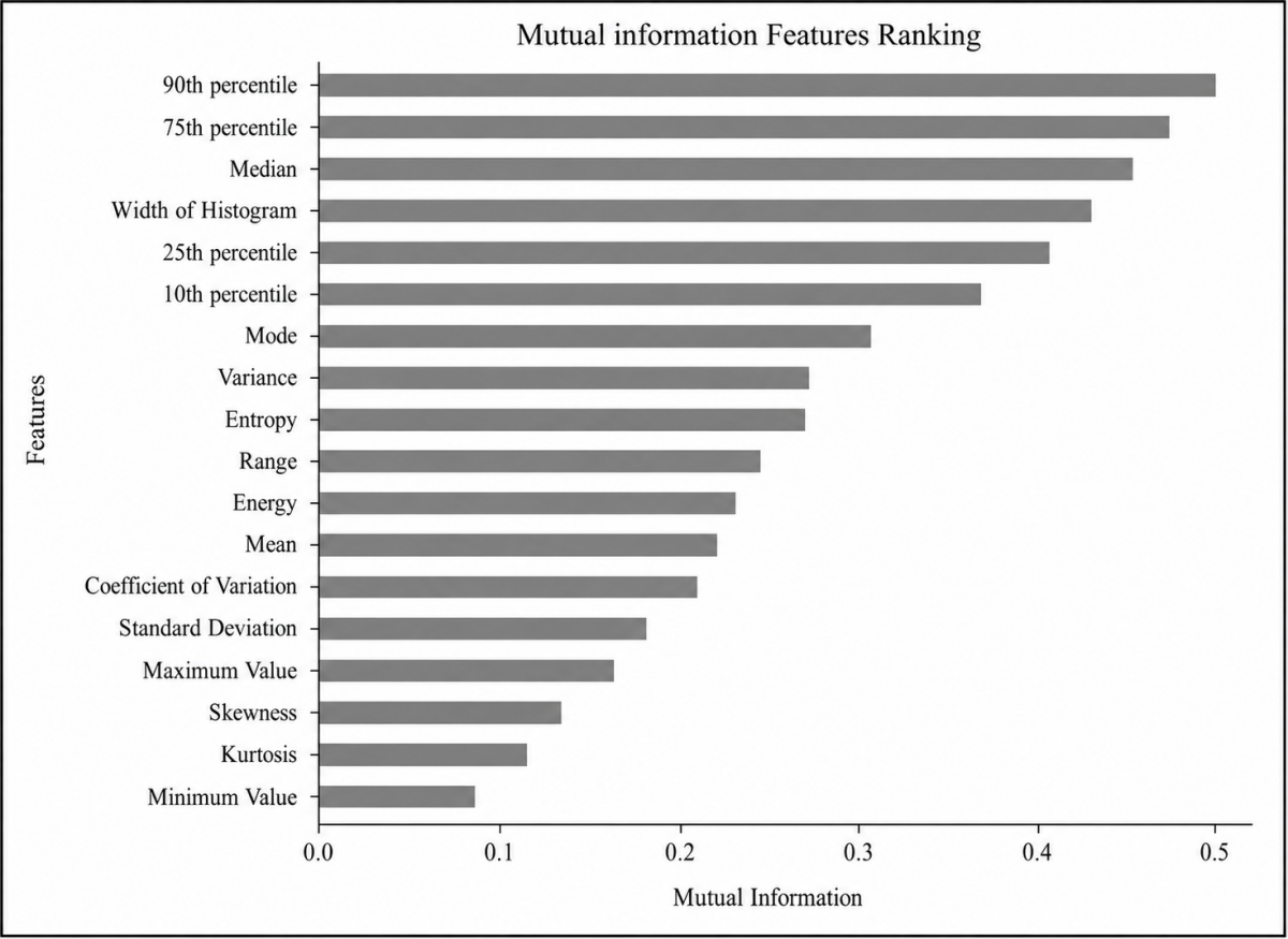
The MI content values are given in Table 4 and Figure 15, from which the values range between 0.526 and 0.094. The highest-ranked feature is the 90th percentile, whereas the lowest-ranked feature is the minimum value.
Table 4. Feature ranking based on mutual information (MI)
|
Feature |
MI |
|
90th percentile |
0.52617 |
|
75th percentile |
0.50563 |
|
Median |
0.48077 |
|
Width of histogram |
0.46100 |
|
25th percentile |
0.43423 |
|
10th percentile |
0.41629 |
|
Mode |
0.36142 |
|
Variance |
0.29201 |
|
Entropy |
0.28956 |
|
Range |
0.25540 |
|
Energy |
0.23739 |
|
Mean |
0.23456 |
|
Coefficient of variation |
0.22194 |
|
Standard deviation |
0.19941 |
|
Maximal value |
0.19409 |
|
Skewness |
0.15512 |
|
Kurtosis |
0.14225 |
|
Minimal value |
0.09406 |
Figure 15. Feature ranking based on mutual information (MI)
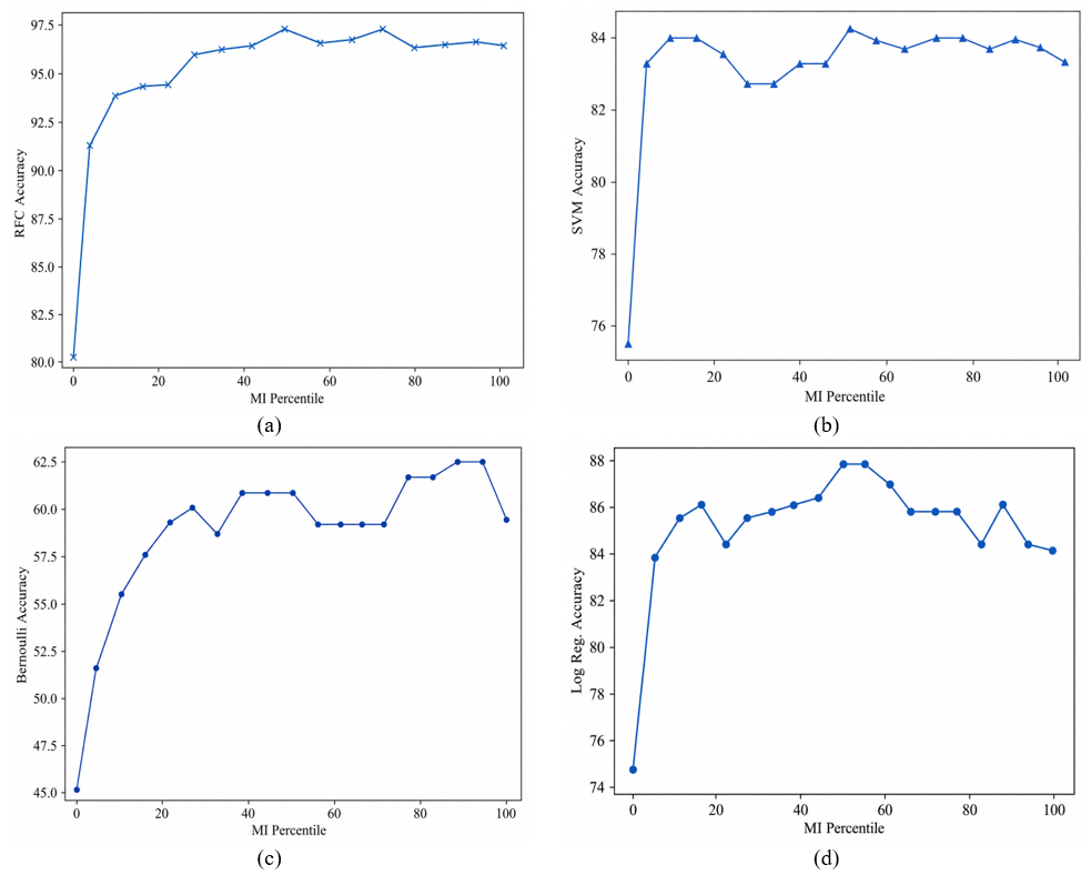
The accuracy of using different percentiles with the four models is illustrated in Figure 16, where Figure 16(a) gives the accuracy using RFC, Figure 16(b) shows the accuracy using SVM, Figure 16(c) gives the accuracy using Bernoulli, and Figure 16(d) gives the accuracy using Logistic Regression. From the graphs in this figure, it is clear that the curves are not monotonically increasing and, in some cases, the increase in the percentile caused a decrease in the accuracy. The majority of the models gave the best result at the 50% percentile, and the best performance was achieved with RFC.
Figure 16. The accuracy of the models according to the percentile: (a) Random Forest Classifier (RFC), (b) Support Vector Machine (SVM), (c) Bernoulli, (d) Logistic Regression
4.7.3 Machine learning
The last feature ranking method used is based on machine learning models, namely, RFC, SVM, Bernoulli, and Logistic Regression models. Each feature is used solely to train the models, and the accuracy is evaluated. Table 5 presents the results obtained using the aforementioned approach to evaluate the features. From the table, it is clear that the best performance was associated with RFC and the worst performance was associated with Bernoulli.
Table 5. The accuracy of the four models used with respect to features
|
Feature |
RFC |
Feature |
SVM |
Feature |
Ber |
Feature |
Log Reg |
|
Width of histogram |
0.942 |
90th percentile |
0.831 |
Median |
0.550 |
90th percentile |
0.829 |
|
90th percentile |
0.914 |
Width of histogram |
0.815 |
Standard deviation |
0.550 |
Entropy |
0.807 |
|
75th percentile |
0.901 |
Entropy |
0.809 |
Mode |
0.544 |
Width of histogram |
0.807 |
|
25th percentile |
0.887 |
Coefficient of variation |
0.790 |
75th percentile |
0.541 |
Variance |
0.801 |
|
Median |
0.884 |
Variance |
0.787 |
Width of histogram |
0.525 |
Coefficient of variation |
0.785 |
|
Mode |
0.848 |
Mean |
0.782 |
10th percentile |
0.519 |
Mean |
0.779 |
|
10th percentile |
0.831 |
Energy |
0.735 |
Range |
0.519 |
Energy |
0.749 |
|
Standard deviation |
0.754 |
75th percentile |
0.710 |
90th percentile |
0.514 |
75th percentile |
0.746 |
|
Variance |
0.738 |
Standard deviation |
0.696 |
25th percentile |
0.511 |
Standard deviation |
0.693 |
|
Entropy |
0.729 |
Skewness |
0.685 |
Coefficient of variation |
0.503 |
Median |
0.691 |
|
Coefficient of variation |
0.715 |
Median |
0.680 |
Energy |
0.503 |
Skewness |
0.691 |
|
Mean |
0.715 |
Kurtosis |
0.657 |
Entropy |
0.503 |
Kurtosis |
0.669 |
|
Energy |
0.713 |
10th percentile |
0.610 |
Kurtosis |
0.503 |
25th percentile |
0.655 |
|
Range |
0.707 |
25th percentile |
0.597 |
Mean |
0.503 |
Mode |
0.649 |
|
Maximum value |
0.663 |
Mode |
0.577 |
Skewness |
0.503 |
10th percentile |
0.613 |
|
Skewness |
0.644 |
Maximum value |
0.541 |
Variance |
0.503 |
Maximum value |
0.544 |
|
Kurtosis |
0.613 |
Range |
0.541 |
Maximum value |
0.494 |
Range |
0.541 |
|
Minimum value |
0.575 |
Minimum value |
0.503 |
Minimum value |
0.481 |
Minimum value |
0.519 |
Note: RFC = Random Forest Classifier, SVM = Support Vector Machine.
4.7.4 Overall feature importance
The final stage is to find the overall feature ranks based on the four aforementioned methods; the final rank can be determined by finding the sum of all ranks. The three methods were used because they assess feature relevance from different perspectives. For instance, correlation analysis measures the statistical association between individual features and the class label, MI quantifies the amount of shared information regardless of linearity, and machine learning-based evaluation assesses the discriminative capability of each feature when used independently. These evaluation measures are therefore considered complementary indicators of feature relevance rather than direct measures of predictive ability. By considering these complementary evaluation criteria together, the proposed framework provides a comprehensive assessment of feature relevance and reduces the possibility of selecting features based on a single evaluation measure. Table 6 lists the overall feature ranks.
Based on the combined evaluation criteria, the features with the highest overall relevance scores were selected for the final classification stage. These features consistently demonstrated stronger statistical association, higher information content, and greater discriminative capability than the remaining features. Their final predictive performance was subsequently validated using the machine learning classifiers.
The proposed approach initially evaluates the features independently to determine their individual importance. However, the final classification models are trained using the selected features as a combined feature vector, allowing the classifiers to implicitly capture the interactions and complementary information among the selected features. Higher-order feature interactions analysis is beyond the scope of this study and is considered for future work.
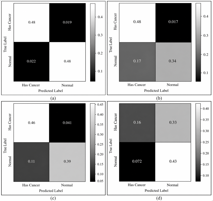
Table 7 and Figure 17 show the results obtained when using the aforementioned features to train the models. Precision/recall/accuracy measures were adopted as they are widely used in the literature. For more information about these measures, please refer to the previous study [1]. From Table 7 and Figure 17, which show the confusion matrices of the four models, we can observe that the best performance was achieved with the RFC, for which the accuracy reached 95.85%.
Table 6. Feature ranking based on the three evaluation methods
|
Feature |
Pearson |
Kendall |
Spearman |
MI |
RFC |
SVM |
Ber |
Log Reg |
All |
|
90th percentile |
0.580 |
0.496 |
0.602 |
0.526 |
0.914 |
0.831 |
0.514 |
0.829 |
5.292 |
|
Width of histogram |
0.555 |
0.508 |
0.618 |
0.461 |
0.942 |
0.815 |
0.525 |
0.807 |
5.231 |
|
Entropy |
0.585 |
0.532 |
0.651 |
0.290 |
0.729 |
0.809 |
0.503 |
0.807 |
4.906 |
|
75th percentile |
0.479 |
0.450 |
0.543 |
0.506 |
0.901 |
0.710 |
0.541 |
0.746 |
4.875 |
|
Coefficient of variation |
0.547 |
0.521 |
0.637 |
0.222 |
0.715 |
0.790 |
0.503 |
0.785 |
4.720 |
|
Variance |
0.517 |
0.474 |
0.580 |
0.292 |
0.738 |
0.787 |
0.503 |
0.801 |
4.692 |
|
Mean |
0.531 |
0.459 |
0.562 |
0.235 |
0.715 |
0.782 |
0.503 |
0.779 |
4.566 |
|
Median |
0.372 |
0.380 |
0.456 |
0.481 |
0.884 |
0.680 |
0.550 |
0.691 |
4.493 |
|
Energy |
0.522 |
0.453 |
0.555 |
0.237 |
0.713 |
0.735 |
0.503 |
0.749 |
4.467 |
|
Standard deviation |
0.367 |
0.326 |
0.396 |
0.199 |
0.754 |
0.696 |
0.550 |
0.693 |
3.982 |
|
Skewness |
0.453 |
0.382 |
0.468 |
0.155 |
0.644 |
0.685 |
0.503 |
0.691 |
3.980 |
|
Kurtosis |
0.408 |
0.388 |
0.475 |
0.142 |
0.613 |
0.657 |
0.503 |
0.669 |
3.856 |
|
25th percentile |
0.215 |
0.240 |
0.289 |
0.434 |
0.887 |
0.597 |
0.511 |
0.655 |
3.826 |
|
10th percentile |
0.186 |
0.262 |
0.312 |
0.416 |
0.831 |
0.610 |
0.519 |
0.613 |
3.751 |
|
Mode |
0.207 |
0.131 |
0.157 |
0.361 |
0.848 |
0.577 |
0.544 |
0.649 |
3.475 |
|
Range |
0.174 |
0.086 |
0.101 |
0.255 |
0.707 |
0.541 |
0.519 |
0.541 |
2.926 |
|
Maximum value |
0.176 |
0.081 |
0.094 |
0.194 |
0.663 |
0.541 |
0.494 |
0.544 |
2.788 |
|
minimum value |
0.051 |
0.081 |
0.086 |
0.094 |
0.575 |
0.503 |
0.481 |
0.519 |
2.390 |
Note: MI = mutual information, RFC = Random Forest Classifier, SVM = Support Vector Machine.
Table 7. Precision, recall, F1-score, and accuracy of the four models using the optimal features
|
Model |
|
Precision |
Recall |
F1-Score |
Accuracy % |
|
RFC |
Normal |
0.96 |
0.96 |
0.96 |
95.85 |
|
Abnormal |
0.96 |
0.96 |
0.96 |
||
|
Macro average |
0.96 |
0.96 |
0.96 |
||
|
Weighted average |
0.96 |
0.96 |
0.96 |
||
|
SVM |
Normal |
0.74 |
0.97 |
0.84 |
81.76 |
|
Abnormal |
0.95 |
0.67 |
0.79 |
||
|
Macro average |
0.85 |
0.82 |
0.81 |
||
|
Weighted average |
0.85 |
0.82 |
0.81 |
||
|
Logistic Regression |
Normal |
0.80 |
0.92 |
0.86 |
84.80 |
|
Abnormal |
0.90 |
0.78 |
0.84 |
||
|
Macro average |
0.85 |
0.85 |
0.85 |
||
|
Weighted average |
0.85 |
0.85 |
0.85 |
||
|
Bernoulli |
Normal |
0.69 |
0.33 |
0.45 |
59.39 |
|
Abnormal |
0.56 |
0.86 |
0.68 |
||
|
Macro average |
0.63 |
0.59 |
0.56 |
||
|
Weighted average |
0.63 |
0.59 |
0.56 |
Note: RFC = Random Forest Classifier, SVM = Support Vector Machine.
Figure 17. Confusion matrix of the models: (a) Random Forest Classifier (RFC), (b) Support Vector Machine (SVM), (c) Logistic Regression, and (d) Bernoulli
Table 8. Results benchmarking
|
# |
Research |
Approach |
Dataset |
Number of Images |
Accuracy % |
|
1. |
ELD [21] |
PCA, KNN |
Harvard Medical School (HMS) |
70, 10 normal and 60 abnormal |
98 |
|
2. |
ZO [22] |
SVM |
Bayer Schering Pharma dataset (BSP) |
101 |
85 |
|
3. |
ZN [23] |
FMC, SRG, JSC |
- |
- |
90 |
|
4. |
CUI [24] |
LFC |
- |
- |
83 to 95 |
|
5. |
SAC [25] |
ANN PCA-ANN |
Custom |
55 patients |
77 to 91 |
|
6. |
ELD [26] |
PCNN |
Harvard Medical School (HMS) |
101, 14 normal and 87 abnormal |
99 |
|
7. |
KV [27] |
PCA, RBF, SVM |
Harvard Medical School (HMS) |
- |
94 |
|
8. |
DR [28] |
ANN |
- |
- |
85 |
|
9. |
AM [29] |
K-means, SOM-NN, KNN |
Custom |
40 60 70 |
85 96. 6 94. 28 |
|
10. |
BAH-1 [30] |
BWT, SVM, ANFIS, BP-ANN, KNN |
Custom |
135 images of 15 patients |
80.29 to 96.51 |
|
11. |
GIL [31] |
Gabor, SVM |
Harvard Medical School (HMS) |
101, 14 normal/ 87 abnormal 75, 15 normal/ 60 abnormal 70, 10 normal/ 60 abnormal |
100 100 100 |
|
12. |
BAH-2 [32] |
GA |
Custom Digital Imaging and Communications in Medicine (DICOM) Brain Web dataset (BWD) |
15 patients 22
44 |
92.03 |
|
13. |
OZ [33] |
CNN and SVM CNN and KNN |
Cancer Genome Atlas (TCGA) |
500 |
93.1 87.5 |
|
14. |
RZ [34] |
machine-learning classification |
Public brain MRI datasets |
7023 |
95.56 |
|
15. |
TM [35] |
KNN, SVM and neural-network classifiers |
Public brain MRI dataset |
660 |
95.86 |
|
16. |
KK [36] |
HOG, LBP and image-based feature representations with RF, SVM, LR, KNN, NB and DT |
Two public Kaggle MRI datasets |
Not clearly stated |
99.00 |
|
17. |
MM [37] |
Statistical and CNN-derived features with one-class SVM |
Public binary brain MRI dataset |
Not clearly stated |
94.83 |
|
18. |
Proposed |
Symmetry, FOS-RFC |
|
3053 |
95.85 |
Note: PCA = Principal Component Analysis; KNN = K-Nearest Neighbors; SVM = Support Vector Machine; FMC = Fuzzy Mean Clustering; SRG = Seeded Region Growing; JSC = Joint Sparse Coding; LFC = Local Feature Clustering; ANN = Artificial Neural Network; PCA-ANN = Principal Component Analysis–Artificial Neural Network; PCNN = Pulse-Coupled Neural Network; RBF = Radial Basis Function; SOM-NN = Self-Organizing Map–Neural Network; BWT = Backward Weight Transfer; ANFIS = Adaptive Neuro-Fuzzy Inference System; BP-ANN = Backpropagation Artificial Neural Network; GA = Genetic Algorithm; CNN = Convolutional Neural Network; HOG = Histogram of Oriented Gradients; LBP = Local Binary Pattern; RF = Random Forest; LR = Logistic Regression; KNN = K-Nearest Neighbors; NB = Naive Bayes; DT = Decision Tree; RFC = Random Forest Classifier; MRI = magnetic resonance imaging, FOS = first-order statistics.
4.8 Benchmarking
The results obtained in this study were benchmarked with the following some state-of-the-art methods: El-Dahshan et al. (ELD) [21], Zöllner et al. (ZO) [22], Zanaty (ZN) [23], Cui et al. (CUI) [24], Sachdeva et al. (SAC) [25], El-Dahshan et al. (ELD) [26], Kumar and Vijayakumar (KV) [27], Damodharan and Raghavan (DR) [28], Anitha and Murugavalli (AM) [29], Bahadure et al. (AM) [30], Gilanie et al. (GIL) [31], Bahadure et al. (BAH-2) [32], Özyurt et al. (OZ) [33], Rasheed et al. (RZ) [34], Tahosin et al. (TM) [35], Kumar et al. (KK) [36], and Mjahad and Munaz (MM) [37].
In our discussion, we mainly considered the accuracy and number of images used in the dataset to benchmark our results using the selected methods. From Table 8, it is clear that the proposed algorithm has provided very good accuracy values with RFC. Although some methods have reported accuracy values above 95% and some reached 100%, such as ELD [21], ELD [26], AM [29], and GIL [31], there is a certain limitation with these algorithms, which is the small number of images used in testing, where the number of images was 70, 101, 60, and 101, 75, and 70 images, respectively.
The proposed framework achieved a competitive accuracy using a consolidated dataset of 3,053 MRI images, which indicates the robustness of the proposed approach. Nevertheless, the comparative results should be interpreted in the context of differences in dataset composition, MRI sequences, preprocessing procedures, class distributions, and evaluation protocols. Based on that, Table 8 is intended to demonstrate the competitiveness of the proposed method within the reported literature rather than provide a strictly controlled head-to-head comparison.
This study demonstrated the effectiveness of symmetry-based analysis combined with FOS features in detecting brain abnormalities using MRI images. By evaluating 18 statistical metrics through correlation, MI, and machine learning-based methods, the research identified the most impactful features for classification. The integration of these selected features with an RFC achieved a high accuracy of 95.85%. The proposed approach achieves competitive performance compared with many state-of-the-art approaches, particularly considering the larger dataset used. The results validate the potential of symmetry-driven, feature-optimised CAD systems in supporting reliable and scalable brain abnormality detection. Future work may explore the incorporation of higher-order statistical features and deep learning models to further enhance diagnostic precision.
The utilisation of a consolidated dataset constructed from diverse public MRI datasets has provided greater variability and diversity than a single-source dataset and has enhanced the robustness of the proposed framework by testing it under more heterogeneous conditions. Future work will focus on validating the proposed method using additional independent clinical and multi-centre MRI datasets.
From a practical perspective, the proposed framework can be integrated into CAD systems as an automated decision-support module for brain MRI analysis. By exploiting bilateral brain symmetry and a compact set of discriminative FOS features, the framework can assist radiologists in identifying suspicious abnormalities, prioritizing cases for further examination, and improving diagnostic consistency while maintaining low computational complexity.
Beyond its classification performance, the proposed framework demonstrates the applicability of intelligent information processing techniques to medical image analysis. The proposed symmetry-based framework provides an efficient and interpretable approach that can support CAD and future medical information systems for automated brain MRI analysis.
[1] Al-Azawi, M.A.N. (2023). Symmetry-based brain abnormality identification in magnetic resonance images (MRI). Multimedia Tools and Applications, 82(2): 2563-2586. https://doi.org/10.1007/s11042-022-12197-4
[2] Al-Azawi, M. (2021). Saliency-based brain abnormality identification in magnetic resonance images. Scientific Visualization, 13(2): 24-49. https://doi.org/10.26583/sv.13.2.03
[3] Hu, X.Y., Rajendran, L., Lapointe, E., et al. (2019). Three-dimensional MRI sequences in MS diagnosis and research. Multiple Sclerosis Journal, 25(13): 1700-1709. https://doi.org/10.1177/1352458519848100
[4] Li, Q., Yu, Z., Wang, Y., Zheng, H. (2020). TumorGAN: A multi-modal data augmentation framework for brain tumor segmentation. Sensors, 20(15): 4203. https://doi.org/10.3390/s20154203
[5] Tomasila, G., Rahardjo Emanuel, A.W. (2020). MRI image processing method on brain tumors: A review. AIP Conference Proceedings, 2296(1): 020023. https://doi.org/10.1063/5.0030978
[6] Mohammed, Y.M.A., El Garouani, S., Jellouli, I. (2023). A survey of methods for brain tumor segmentation-based MRI images. Journal of Computational Design and Engineering, 10(1): 266-293. https://doi.org/10.1093/JCDE/QWAC141
[7] Ghorbian, M., Ghorbian, S., Ghobaei-Arani, M. (2024). A comprehensive review on machine learning in brain tumor classification: Taxonomy, challenges, and future trends. Biomedical Signal Processing and Control, 98: 106774. https://doi.org/10.1016/J.BSPC.2024.106774
[8] Iratni, M., Abdullah, A., Aldhaheri, M., et al. (2025). Transformers for neuroimage segmentation: Scoping review. Journal of Medical Internet Research, 27: e57723. https://doi.org/10.2196/57723
[9] Valverde, J.M., Imani, V., Abdollahzadeh, A., et al. (2021). Transfer learning in magnetic resonance brain imaging: A systematic review. Journal of Imaging, 7(4): 66. https://doi.org/10.3390/jimaging7040066
[10] Netshamutshedzi, N., Netshikweta, R., Ndogmo, J.C., Obagbuwa, I.C. (2025). A systematic review of the hybrid machine learning models for brain tumour segmentation and detection in medical images. Frontiers in Artificial Intelligence, 8: 1615550. https://doi.org/10.3389/frai.2025.1615550
[11] Dorfner, F.J., Patel, J.B., Kalpathy-Cramer, J., Gerstner, E.R., Bridge, C.P. (2025). A review of deep learning for brain tumor analysis in MRI. npj Precision Oncology, 9: 2. https://doi.org/10.1038/s41698-024-00789-2
[12] Khalighi, S., Reddy, K., Midya, A., Pandav, K.B., Madabhushi, A., Abedalthagafi, M. (2024). Artificial intelligence in neuro-oncology: Advances and challenges in brain tumor diagnosis, prognosis, and precision treatment. npj Precision Oncology, 8: 80. https://doi.org/10.1038/s41698-024-00575-0
[13] Vergara, J.R., Estévez, P.A. (2014). A review of feature selection methods based on mutual information. Neural Computing and Applications, 24(1): 175-186. https://doi.org/10.1007/s00521-013-1368-0
[14] Pascoal, C., Oliveira, M.R., Pacheco, A., Valadas, R. (2017). Theoretical evaluation of feature selection methods based on mutual information. Neurocomputing, 226: 168-181. https://doi.org/10.1016/j.neucom.2016.11.047
[15] Mielniczuk, J. (2022). Information theoretic methods for variable selection—A review. Entropy, 24(8): 1079. https://doi.org/10.3390/e24081079
[16] Feltrin, F. (2023). Brain tumor MRI images. Kaggle. https://www.kaggle.com/datasets/fernando2rad/brain-tumor-mri-images-44c.
[17] Pradeep. (2022). Brain MRI. Kaggle. https://www.kaggle.com/datasets/pradeep2665/brain-mri.
[18] Yeaf, A. (2023). Brain MRI images. Kaggle. https://www.kaggle.com/datasets/ashfakyeafi/brain-mri-images.
[19] Bhuvaji, S., Kadam, A., Bhumkar, P., Dedge, S., Kanchan, S. (2025). Brain tumor classification (MRI). Kaggle. https://doi.org/10.34740/KAGGLE/DSV/12745533
[20] Al-Azawi, M. (2022). Brain cancer MRI images, lobes symmetry dataset. Kaggle. https://doi.org/10.34740/KAGGLE/DSV/4710773
[21] El-Dahshan, E.S.A., Hosny, T., Salem, A.B.M. (2010). Hybrid intelligent techniques for MRI brain images classification. Digital Signal Processing, 20(2): 433-441. https://doi.org/10.1016/j.dsp.2009.07.002
[22] Zöllner, F.G., Emblem, K.E., Schad, L.R. (2012). SVM-based glioma grading: Optimization by feature reduction analysis. Zeitschrift für Medizinische Physik, 22(3): 205-214. https://doi.org/10.1016/j.zemedi.2012.03.007
[23] Zanaty, E.A. (2012). Determination of gray matter (GM) and white matter (WM) volume in brain magnetic resonance images (MRI). International Journal of Computer Applications, 45(3): 16-22. https://doi.org/10.5120/6759-9021
[24] Cui, W., Wang, Y., Fan, Y., Feng, Y., Lei, T. (2013). Localized FCM clustering with spatial information for medical image segmentation and bias field estimation. International Journal of Biomedical Imaging, 2013: 930301. https://doi.org/10.1155/2013/930301
[25] Sachdeva, J., Kumar, V., Gupta, I., Khandelwal, N., Ahuja, C.K. (2013). Segmentation, feature extraction, and multiclass brain tumor classification. Journal of Digital Imaging, 26(6): 1141-1150. https://doi.org/10.1007/s10278-013-9600-0
[26] El-Dahshan, E.A.S., Mohsen, H.M., Revett, K., Salem, A.B.M. (2014). Computer-aided diagnosis of human brain tumor through MRI: A survey and a new algorithm. Expert Systems with Applications, 41(11): 5526-5545. https://doi.org/10.1016/j.eswa.2014.01.021
[27] Kumar, P., Vijayakumar, B. (2015). Brain tumour MR image segmentation and classification using by PCA and RBF kernel based support vector machine. Middle-East Journal of Scientific Research, 23(9): 2106-2116. https://doi.org/10.5829/idosi.mejsr.2015.23.09.22458
[28] Damodharan, S., Raghavan, D. (2015). Combining tissue segmentation and neural network for brain tumor detection. The International Arab Journal of Information Technology, 12(1): 42-52. https://www.ccis2k.org/iajit/PDF/vol.12,no.1/5430.pdf.
[29] Anitha, V., Murugavalli, S. (2016). Brain tumour classification using two-tier classifier with adaptive segmentation technique. IET Computer Vision, 10(1): 9-17. https://doi.org/10.1049/iet-cvi.2014.0193
[30] Bahadure, N.B., Ray, A.K., Thethi, H.P. (2017). Image analysis for MRI based brain tumor detection and feature extraction using biologically inspired BWT and SVM. International Journal of Biomedical Imaging, 2017: 9749108. https://doi.org/10.1155/2017/9749108
[31] Gilanie, G., Bajwa, U.I., Waraich, M.M., Habib, Z., Ullah, H., Nasir, M. (2018). Classification of normal and abnormal brain MRI slices using Gabor texture and support vector machines. Signal, Image and Video Processing, 12(3): 479-487. https://doi.org/10.1007/s11760-017-1182-8
[32] Bahadure, N.B., Ray, A.K., Thethi, H.P. (2018). Comparative approach of MRI-based brain tumor segmentation and classification using genetic algorithm. Journal of Digital Imaging, 31(4): 477-489. https://doi.org/10.1007/s10278-018-0050-6
[33] Özyurt, F., Sert, E., Avci, E., Dogantekin, E. (2019). Brain tumor detection based on convolutional neural network with neutrosophic expert maximum fuzzy sure entropy. Measurement, 147: 106830. https://doi.org/10.1016/j.measurement.2019.07.058
[34] Rasheed, Z., Ma, Y. K., Ullah, I., et al. (2023). Brain tumor classification from MRI using image enhancement and convolutional neural network techniques. Brain Sciences, 13(9): 1320. https://doi.org/10.3390/brainsci13091320
[35] Tahosin, M.S., Sheakh, M.A., Islam, T., Lima, R.J., Begum, M. (2023). Optimizing brain tumor classification through feature selection and hyperparameter tuning in machine learning models. Informatics in Medicine Unlocked, 43: 101414. https://doi.org/10.1016/j.imu.2023.101414
[36] Kumar, K., Jyoti, K., Kumar, K. (2024). Machine learning for brain tumor classification: Evaluating feature extraction and algorithm efficiency. Discover Artificial Intelligence, 4: 112. https://doi.org/10.1007/s44163-024-00214-4
[37] Mjahad, A., Rosado-Muñoz, A. (2025). Optimizing tumor detection in brain MRI with one-class SVM and convolutional neural network-based feature extraction. Journal of Imaging, 11(7): 207. https://doi.org/10.3390/jimaging11070207