Kunj Modi | Hitansh Mehta | Vidit Thakkar | Darshana Sankhe | Paresh Nasikkar* | Ankita Gupta | Deepali Patil | Pratik Kanani
© 2026 The authors. This article is published by IIETA and is licensed under the CC BY 4.0 license (http://creativecommons.org/licenses/by/4.0/).
OPEN ACCESS
Inventory control in multi-echelon supply chains remains challenging due to stochastic demand, uncertain lead times, and the coupling between production and procurement decisions. This study proposes a cooperative Multi-Agent Reinforcement Learning (MARL) framework for two-echelon inventory management, where finished-goods production and raw-material procurement are modeled as interacting decision-making agents under a shared cost-minimization objective. A two-stage training strategy is developed by combining behavioral cloning (BC) from heuristic demonstrations with Proximal Policy Optimization (PPO) fine-tuning. In addition, a monotonicity-based regularization term is introduced into the PPO objective to incorporate fundamental inventory principles and improve policy consistency. The proposed framework is evaluated in a simulated multi-product inventory environment and compared with a dynamic base-stock policy. Experimental results demonstrate an improvement in total system cost of 2.2% for the learned policy while maintaining a service level of 99.1%, between inventory holding costs and shortage risks. Further analyses, including ablation studies and disruption scenarios, where demonstration-based initialization and monotonicity constraints contribute to more stable and economically reasonable decision policies. The proposed approach provides a data-driven solution for adaptive inventory control in complex supply chain systems.
Multi-Agent Reinforcement Learning, inventory control, two-echelon supply chains, behavioral cloning, Proximal Policy Optimization, adaptive decision-making
A supply chain consists of customers and suppliers working together to deliver finished products to end customers, beginning with raw materials (RMs). Its primary goal is to maintain product availability while minimizing inventory holding costs and the amount of capital tied up in stock [1]. A major challenge is the lack of effective, data-driven information systems (IS) for inventory management. Poor inventory decisions can lead to excessive holding costs and capital tied up in surplus stock, while shortages may result in lost sales and customer dissatisfaction. Recent research has shown that predictive analytics, real-time operational data, and intelligent decision-support technologies can support more responsive inventory planning and reduce both overstocking and critical shortages [2]. As global markets become increasingly volatile, intelligent Enterprise Resource Planning (ERP) modules are becoming increasingly important for managing inventory-related risks and the opportunity costs associated with stock shortages. Under such conditions, the effectiveness of conventional static inventory models is significantly reduced [1].
In this context, Deep Reinforcement Learning (DRL) has emerged as a strong method to solve challenging decision-making problems in a sequential setting under uncertainty [3]. Different from classical optimization or supervised learning, DRL agents learn an effective control policy by interacting with a dynamic environment through trial and error [4]. Therein lies the exceptional suitability of DRL for engineering modern enterprise systems, allowing the development of adaptive, data-driven IS architectures that autonomously process supply chain data streams to outperform conventional heuristics [3].
A multi-echelon supply chain-with its naturally distributed decision points and interdependencies is best conceptualized as a Multi-Agent Reinforcement Learning (MARL) problem [5]. Decisions at one level, such as Finished Goods (FGs) production, create a demand signal and constraints for other preceding levels, such as RM procurement. Such a system modeled by distinct, interacting agents captures the decentralized reality of supply chain operations [5]. This study considers a cooperative setting in which the agents share a common objective: the minimization of the total system-wide costs. The alignment is enforced through a unified reward signal that compels agents to learn coordinated strategies benefiting the whole system rather than optimizing their local objectives in isolation [6].
In this study, we present a comprehensive framework for a cooperative MARL system as a control module for enterprise IS. It targets specifically two-echelon, multi-product inventory networks. The primary contributions of this research are fourfold:
(1). It formalizes the two-echelon inventory problem as a Multi-Agent Markov Decision Process (MAMDP) where a unified shared reward signal based on the total system cost enforces the collaboration between the FG and RM agents.
(2). It proposes a two-stage "imitate-then-fine-tune" curriculum for training, where behavioral cloning (BC) first pre-trains the agent policy on demonstrations from the heuristic expert, which alone significantly accelerates convergence and stabilizes the subsequent phase of reinforcement learning [7].
(3). It incorporates a structure-based monotonicity regularization into the Proximal Policy Optimization (PPO) loss, embedding key domain knowledge directly inside the learning process [8].
(4). It demonstrates via tests that the trained multi-agent policy outperforms a strong dynamic base-stock baseline, cutting total system cost by 2.2%, accomplishing a better balance between the inventory holding costs and service levels.
While inventory optimization is traditionally based on isolated mathematical models, modern enterprise IS require dynamic modules that are driven by data. This study fills this gap and proposes a MARL framework that is specifically made and tailored to act as an intelligent control layer for these enterprise systems (e.g., SAP Integrated Business Planning), converting raw streams of supply chain data into automated, coordinated decisions that help with procurement and production.
The Economic Order Quantity (EOQ) model, which was first introduced in 1913, attempts to minimize the sum of the holding costs and the ordering costs [9]. Base-stock policies, which are optimal when there is no uncertainty, are not effective in managing a modern supply chain, which consists of stochastic demand and lead times as well as complex relations between products and supply chain steps [1].
The bullwhip effect increases the impact of order changes in multi-level structures and introduces control problems [10]. In planning multi-item systems, using heuristics as in METRIC leads to bad results in case of high variability [11]. Recent planning approaches use stochastic programming or robust optimization to account for variability. However, most of these methods are not applicable for large numbers of items [12].
Reinforcement learning is powerful for finding near-optimal policies for stock, work-in-process inventory, and broader Supply Chain Management (SCM) problems [1]. Deep Q-Networks (DQN), Deep Deterministic Policy Gradient (DDPG), Asynchronous Advantage Actor-Critic (A3C), and others have led to policies for corresponding rule-based systems that are dramatically better [10]. A simple example is a single-level inventory problem with lost sales, approximated by finding near-optimal (s, S) policies in a relevant portion of the state space and corresponding inventory positions using DQN in a simulated retail environment, which resulted in costs down 20% [13]. In problems with continuous actions, the Deterministic Policy Gradient (DDPG) can be used. Recently, such a method has been used for finding lot-sizing policies, given a fixed, limited production capacity that can be used to adapt to changes in demand [14].
Supply chain management has recently started to be tackled using MARL in order to better model and understand the complex behavior of supply chains [5]. By modeling the interactions of the different players (e.g., manufacturers, distributors, retailers) that are part of a supply chain, MARL can capture system-wide effects and strive to achieve system-wide goals, in contrast to single-agent methods, which only provide a partial solution for managing supply chains. Cooperative MARL is trained using a method of centralized training with decentralized execution (CTDE) [15]. It reduces the bullwhip effect in serial supply chains by up to 15–30%.
By utilizing BC, sample efficiency and training time are greatly improved [16]. For SCM, by first initializing meaningful behavior for RL agents by utilizing BC in combination with heuristic experts (e.g., base-stock policies) for RL agents, such agents are prevented from engaging in an inordinate amount of exploration in environments where rewards are very sparse [17].
The monotonicity constraints, enforcing increase in demand leads to an increase in order quantities, are compatible with the usual tenets of inventory theory, such as the well-known Clark-Scudder rules [9]. Work in this area that has incorporated such penalties in the form of automatic differentiation in policy gradients has developed very interpretable policies without any corresponding loss in performance [18].
PPO retains the theoretical advantages of trust-region methods like Trust Region Policy Optimization (TRPO) [19] by strictly clipping policy updates to prevent catastrophic performance collapse, but is significantly simpler to implement using only first-order optimization, making it highly suitable for complex, continuous action spaces like those found in inventory ordering tasks [20].
Recent extensions of PPO to SCM include applications to economic dispatch [21] and lot-sizing problems [22], highlighting its versatility in handling stochastic constraints. In multi-agent setups, PPO has been adapted for cooperative tasks such as the control of traffic signals, where shared rewards make the coordination of agents straightforward [23].
Recent MARL literature includes value-decomposition methods such as Monotonic Value Function Factorisation (QMIX) [15] and multi-agent actor-critic methods such as Multi-Agent Proximal Policy Optimization (MAPPO) [24] for problems that need continuous control. When applied to complex supply chain domains, standard algorithms can yield unstable policies that violate fundamental principles of inventory economics. In these cases, domain knowledge is directly encoded by imposing monotonicity regularization on the PPO objective. This ensures the learned policy remains structurally sound while outperforming standard, unregularized MAPPO and QMIX baselines.
This section presents our complete description of the problem along with the framework, methodologies, and datasets that we use to tackle it. We formalize the problem as a MAMDP, describe the simulation environment in which it will be trained and evaluated, detail the underlying neural network architecture and policies, and finally present a two-step training framework combining Behavioural Cloning with PPO.
3.1 Problem formulation as a cooperative Multi-Agent Markov Decision Process
The proposed inventory management solution is formulated as a cooperative MAMDP, driven by two distinct policies.
3.1.1 Agents
FG agent. Responsible for production planning. At each daily timestep, it determines the quantity of each of the five distinct finished products to begin producing, subject to RM availability forecasts.
RM agent. Manages procurement. At each daily timestep, it decides the quantity of the single, shared RM to order from an external supplier, aggregating FG signals.
3.1.2 State space
A direct feature engineering approach was adopted to enhance training stability [25].
FG agent state (dim = 37). On-hand FG Inventory (5 dims), FG Production Pipeline (15 dims, 3 stages × 5 products), Demand Metrics (4 dims: current, forecast mean/std, trend), Historical Patterns (3 dims: 7-day avg demand/production/shortage).
Production Metrics (4 dims: RM coverage, backlog), RM Coverage Ratio (1 dim), Temporal Features (2 dims: sin(2πt/365), cos), RM Availability (3 dims: on-hand, pipeline total, lead time est).
RM agent state (dim = 20). On-hand RM Inventory (1 dim), RM Procurement Pipeline (5 dims, stages 1–5), Production Signals (4 dims: aggregated FG orders forecast), Aggregated Demand Metrics (4 dims), Historical Patterns (3 dims), System State Features (3 dims: total FG backlog, cost summary).
States are normalized to [–1, 1] using running statistics.
The state space integrates "Historical Patterns" to allow the agents to perceive recent demand volatility. Let $D_\tau=$ $\sum_{j=1}^M d_{j, \tau}$ represent the total aggregate demand across all $M$ products on day $\tau$. For any current timestep t , the historical patterns feature vector $H_t \in \mathbb{R}^3$ is derived from the preceding 7-day window and comprises the maximum, mean, and standard deviation of total demand:
$H_t=\left[\max _{i \in\{1, \ldots, 7\}} D_{t-i}, \frac{1}{7} \sum_{i=1}^7 D_{t-i}, \sqrt{\frac{1}{7} \sum_{i=1}^7\left(D_{t-i}-\bar{D}\right)^2}\right]$ (1)
3.1.3 Action space
FG agent. Continuous vector of size $5, a_{F G} \in R_{\geq 0}^5$, where each element is the production quantity for a specific product, clipped [0, 20].
RM agent. Continuous scalar, $a_{R G} \in R_{\geq 0}$, representing the procurement quantity for the RM, clipped to $[0,50]$.
Actions are executed sequentially: FG first (signals RM demand), then RM.
The continuous actions produced by the actor networks, denoted as $a_{J, t}^{\widetilde{F G}}$ for the FG agent and $a_t^{\widetilde{R M}}$ for the RM agent, undergo a multi-step bounding process before environment execution.
For the RM agent, the procurement action is bounded below by zero: $a_t^{R M}=\max \left(0, \widetilde{a_t^{R M}}\right)$.
For the FG agent, actions are subjected to a dynamic scaling mechanism based on the available RM inventory to prevent infeasible production plans. The raw actions are first clipped for non-negativity: $a_{j, t}^{\prime}=\max \left(0, \widetilde{a_{J, t}^{F G}}\right)$. Next, a dynamic scaling factor $\beta$ is computed using a threshold of 1.5 times the current RM inventory:
$\beta=\min \left(1, \frac{1.5 \cdot I_t^{R M}}{\sum_{j=1}^M a_{j, t}^{\prime}}\right)$ (2)
Finally, the actions are scaled and clipped to a maximum physical production capacity of 25 units per product:
$a_{j, t}^{F G}=\operatorname{clip}\left(\beta \cdot a_{j, t}^{\prime}, 0,25\right)$ (3)
3.1.4 Reward function
To ensure strict cooperation, both the FG and RM agents receive an identical, unified reward signal at each timestep t, defined as the negative of the total system costs. The reward function incorporates a smooth quadratic penalty for RM stockouts to ensure stable policy gradients during training. The aggregate unified reward $r_t$ is:
Unified reward.
$\begin{aligned} r_t=-\left(C_{\text {holding}, t}^{F G}\right. & +C_{\text {shortage}, t}^{F G}+C_{\text {holding}, t}^{R M}\left.+C_{\text {order}, t}^{R M}+C_{\text {penalty}, t}^{R M}\right)\end{aligned}$ (4)
FG holding cost.
$C_{\text {holding}, t}^{F G}=\sum_{j=1}^M h_j^{F G} I_{j, t}^{F G}$ (5)
FG shortage cost.
$C_{\text {shortage}, t}^{F G}=\sum_{j=1}^M \pi_j^{F G} \max \left(0, d_{j, t}-I_{j, t}^{F G}\right)$ (6)
RM holding cost.
$C_{\text {holding}, t}^{R M}=h^{R M} I_t^{R M}$ (7)
RM ordering cost.
$C_{\text {order }, t}^{R M}=K^{R M} \cdot \mathbb{I}\left(a_t^{R M}>0\right)$ (8)
An RM stockout penalty is imposed whenever the production plan exceeds the available RM inventory. Let $\rho_t=$ $\max \left(0, \sum_{j=1}^M a_{j, t}^{F G}-I_t^{R M}\right)$ be the shortage in RM. Linear and quadratic terms are used to provide smoother gradients:
$C_{\text {penalty}, t}^{R M}=w_1 \rho_t+w_2 \rho_t^2$ (9)
where, $w_1=1.0$ and $w_2=0.5$.
3.2 Simulation environment details
The environment models a two-echelon system consisting of 5 distinct FG products produced from a single RM, with key simulation parameters summarized in Table 1.
Demand generation. Daily demand for each product is sampled from a normal distribution with mean $\mu=5.0$ units/ product/day and standard deviation $\sigma=2.0$ units/ product/day. Demands are clipped to non-negative integers to reflect real-world operational constraints. A 7-day rolling forecast is computed using exponential smoothing $(\alpha=0.3)$.
Lead times. FG production lead time $L_{F G}=3$ days (deterministic); RM procurement lead time $L_{R M}=3$ days (stochastic, uniform [3, 7] days).
Costs. Holding costs $h_{F G}=1.0 /$ unit $/$ day, $h_{R M}=1.0 /$ unit / day; Shortage cost $\pi=1.0 /$ unit; Ordering cost fixed $K_{R M}=50$ /order (FG production cost-free).
Trajectory length. Every episode is 200 timesteps, or days, in length; a total of 1,000 episodes were used for training, with 600-step rollouts for evaluation to obtain an estimate of long-term stability.
State features. The raw simulation data is feature-engineered into states as follows: inventory levels, pipeline contents, demand forecasts (7d rolling window), historical summaries (7d ago), temporal encodings (sin/cos for seasonality). Total state dims: FG = 37, RM = 20.
Table 1. Key simulation parameters
|
Parameter |
Value |
Description |
|
Products |
5 |
FG variants |
|
Demand µ/σ |
5/2 |
Per product/day |
|
$L_{F G}$ |
3 days |
Fixed |
|
$L_{R M}$ |
[3, 7] days |
Stochastic |
|
$h_{F G} / h_{R M}$ |
1.0/0.5 |
Holding costs |
|
π |
10.0 |
Shortage penalty |
3.3 Data augmentation
A dataset comprising approximately 2,000 state-action pairs was generated by rolling out the dynamic base-stock heuristic policy in the environment. The heuristic sets base-stock levels as
$S_j=\mu_j \times\left(L+z \cdot \sigma_j \sqrt{L}\right)$ (10)
where, z = 1.65 corresponds to a 95% service level [26]. Actions in this dataset are normalized to the range [0, 20] units for FG and [0, 50] units for RMs to match the action space constraints defined in Section 3.1. This dataset serves as supervised training data for the BC pre-training phase described in Section 3.5.1.
The complete training process encompasses approximately 200,000 timesteps collected across 1,000 episodes of environment interaction. To ensure statistical rigor in performance evaluation, all policies are assessed using 50 independent rollouts, each spanning 600 timesteps. Performance metrics are reported with 95% confidence intervals computed via bootstrap resampling with 1,000 bootstrap iterations.
This simulation-based dataset ensures reproducibility and allows for controlled ablation studies, while mimicking real-world stochasticity. No external real-world datasets were used, as the focus is on methodological innovation in a controlled setting. Future work could integrate real ERP data from sources like SAP simulations [27].
3.4 Agent policy and value architectures
We parameterized the policies and value functions for both agents with an actor-critic architecture [28]. The FG agent and the RM agent share a neural network design scaled for input dimensions.
Network structure. The input layer is followed by a multilayer perceptron (MLP) body with three hidden layers of 256, 128, and 64 units, each using ReLU activation. This produces a latent representation $z \in R^{32}$.
Actor head. From z, the actor computes the mean µ via a linear layer and parameterizes the log-standard deviation $\log \sigma$ (initialized at -0.5 ). Actions are sampled as
$a=\operatorname{softplus}(\mu+\sigma \cdot \epsilon), \epsilon \sim N(0,1)$ (11)
Critic head. The critic maps z to the state-value function $V(s)$ using a linear layer with tanh activation.
We applied orthogonal initialization for initial training stability, the Adam optimizer (lr = 3e−4), and an entropy bonus Sπ to encourage exploration. The resulting parameter count is ~10,000 for each FG and RM agent. This architecture scales well and handles continuous actions effectively.
3.5 Training framework: Proximal Policy Optimization with performance enhancements
A two-stage training protocol is used to improve sample efficiency and embed domain knowledge from a conventional heuristic model for a warm start. The hyperparameter configuration for PPO fine-tuning is detailed in Table 2.
Table 2. Proximal Policy Optimization (PPO) hyperparameters
|
Hyperparameters |
Value |
Description |
|
Batch size |
2048 |
Timesteps per update |
|
Epochs/update |
10 |
PPO epochs |
|
$\varepsilon_{\text {clip }}$ |
0.2 |
Clipping range |
|
$\lambda_{\text {mono }}$ |
0.1 |
Regularization weight |
|
$\gamma$ |
0.99 |
Discount |
|
$\lambda_{\text {GAE }}$ |
0.95 |
GAE param |
|
Algorithm 1. Two-stage training curriculum |
|
Input: Heuristic expert $\pi_{\text {expert}}$, FG actor network $\theta_{F G}$, RM actor network $\theta_{R M}$, environment $\mathcal{E}$ Phase 1: Behavioral cloning (Pre-training) 1: Initialize demonstration dataset $D=\varnothing$ 2: Roll out $\pi_{\text {expert }}$ in $\mathcal{E}$ for 2000 episodes 3: Store $\left(s_t^{F G}, a_t^{F G}, s_t^{R M}, a_t^{R M}\right)$ in $\mathcal{D}$ 4: For epoch = 1 to 120 do: 5: Update $\theta_{F G}$ using MSE loss: $\mathcal{L}_{\mathcal{B} \mathcal{C}}^{\mathcal{F} \mathcal{G}}=\mathbb{E}_{\mathbb{D}}\left[| | \pi_{\theta_{\mathrm{FG}}}\left(\mathrm{~s}_{\mathrm{t}}\right)-\mathrm{a}_{\mathrm{t}}^{\mathrm{FG}}| |^2\right]$ 6: Update $\theta_{R M}$ using MSE loss: $\mathcal{L}_{\mathcal{B} \mathcal{C}}^{\mathcal{R} \mathcal{C}}=\mathbb{E}_{\mathbb{D}}\left[| | \pi_{\theta_{\mathrm{RM}}}\left(\mathrm{~s}_{\mathrm{t}}\right)-\mathrm{a}_{\mathrm{t}}^{\mathrm{RM}}| |^2\right]$ Phase 2: Proximal Policy Optimization (Fine-tuning) 7: Reset actor learning rates to base value (e.g., 3 × 10⁻⁴) 8: For episode = 1 to 1000 do: 9: Calculate exploration probability: $\epsilon=0.8$ if episode ≤ 700 else 0.2 10: For t = 1 to 365 do: 11: With probability $\epsilon$, sample actions with noise; else deterministic 12: Execute joint action, observe unified reward $r_t$ and next state $s_{t+1}$ 13: Store transitions in agent-specific buffers 14: If buffer size $\geq$ UPDATE_TIMESTEPS: 15: Compute Generalized Advantage Estimates (GAE) 16: Update $\theta_{F G}$ and $\theta_{R M}$ using PPO clipped objective + Monotonicity Regularization 17: Return Optimized policies $\pi_{\theta_{F G}}^*, \pi_{\theta_{R M}}^*$ |
The complete two-stage training curriculum, comprising BC pre-training and PPO fine-tuning, is formally outlined in Algorithm 1.
3.5.1 Behavioral cloning from a heuristic expert
This phase initializes actor policies with expert domain knowledge, reducing initial KL divergence during reinforcement learning [7]. First, state-action trajectory pairs (s, a) are collected from 2,000 heuristic rollouts. Actor networks are then pre-trained using Mean Squared Error (MSE) loss for 120 epochs at a lr = 1e−3, while critic networks are randomly initialized.
3.5.2 Structure-informed Proximal Policy Optimization fine-tuning
Following BC, we fine-tune the agent policies using PPO augmented with a novel monotonicity regularization term that encodes domain knowledge directly into the learning objective.
Training procedure. Fine-tuning proceeds for 1,000 episodes with a batch size of 2,048 timesteps per update. During this phase, collected trajectories are processed to compute advantage estimates using Generalized Advantage Estimation (GAE, λ = 0.95), and returns are normalized to reduce gradient variance and improve training stability.
PPO update. Value loss was given as:
$L^{V F}=E\left[\left(V_\theta\left(s_t\right)-\widehat{R}_t\right)^2\right]$ (12)
Policy loss. Clipped surrogate and augmented with monotonicity. For FG actions $\mu_j$ w.r.t. demand $x_j$,
$L_{\text {mono }}=E\left[\sum_j \max \left(-\frac{\delta \mu_j}{\delta x_j}, 0\right)^2\right]$ (13)
Auto-grad. Gradients are computed via automatic differentiation in real-time during tensor operations to evaluate the total loss function:
$L_{\text {total }}=L^{C L I P}-c_1 L^{V F}+c_2 S\left[\pi_\theta\right]\left(s_t\right)+\lambda_{\text {mono }} L_{\text {mono }}$ (14)
where, $c_1=0.5, c_2=0.01$.
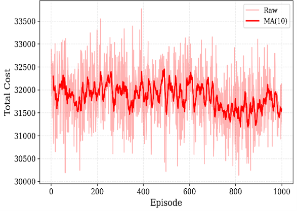
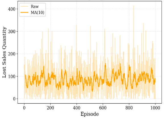
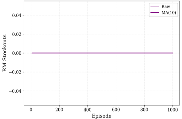
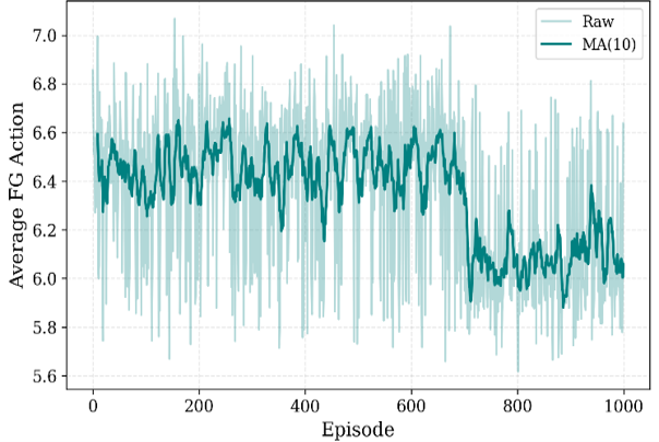
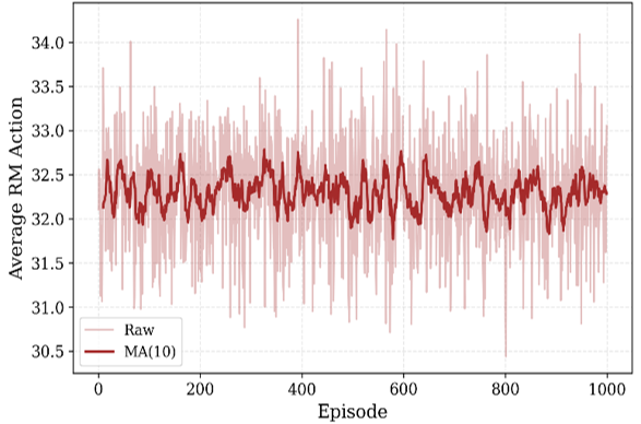
Figure 1 illustrates the evolution of key performance metrics across 1,000 training episodes. The subplots demonstrate policy convergence and behavioral stabilization, confirming the effectiveness of monotonicity regularization in establishing coordinated control strategies.
(a) Episode rewards
(b) Episode costs
(c) Lost sales per episode
(d) Raw Material (RM) stockouts per episode
(e) Average Finished Goods (FG) action per episode
(f) Average Raw Material (RM) action per episode
3.6 Computational efficiency and system requirements
Enterprise supply chain systems require frequent policy retraining under changing market conditions, necessitating computationally lightweight architectures. While many DRL models are heavily GPU accelerated, we were able to successfully train our framework on a normal commercial CPU (Intel Xeon @ 2.20GHz, 13GB RAM). The two-stage curriculum converged at high rates: the BC phase learned the structure of the heuristic at 0.8 seconds, and the PPO fine-tuning reached convergence at 1,000 episodes (approx. 10.6 mins). During inference, a 365-day rollout executes in 0.5188 seconds, demonstrating high computational efficiency. This thus demonstrates the ultra-low computational cost of our framework and the high scalability of our approach. Thus, it can be used for high-frequency and live real-time batch processing of data in live ERP environments without the need for special GPU clusters.
4.1 Comparative performance evaluation
To verify the robustness of the 2.2% cost reduction, statistical significance was evaluated across the 50 independent evaluation rollouts. An independent Welch’s t-test confirmed that the performance difference between the MARL policy and the dynamic base-stock heuristic is statistically significant ($p < 0.001$). Furthermore, bootstrap resampling (1,000 iterations) established a 95% confidence interval for the total cost difference of [–947.42, –422.54], confirming that the framework reliably generates savings and the improvement is not an artifact of random simulation variance.
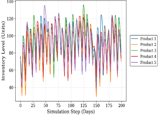
(a) Finished Goods (FG) inventory
(b) Raw Material (RM) inventory
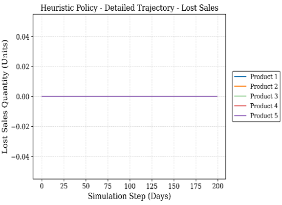
(c) Lost sales
(d) Daily system cost
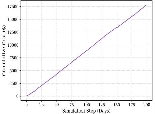
(e) Cumulative system cost
Figure 2 depicts one 200-step rollout for the baseline dynamic base-stock heuristic, with subplots of the FG and RM inventories, lost sales, total step costs, and cumulative system costs. It reflects high volatility in inventories, such as FG spiking to 140 units, and escalating cumulative costs at about 17,600, highlighting the baseline's inability to efficiently manage stochastic demand and maintain an optimal trade-off between holding and shortage costs.
(a) Finished Goods (FG) inventory
(b) Raw Material (RM) inventory
(c) Lost sales
(d) Daily system cost
(e) Cumulative system cost
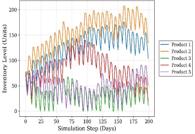
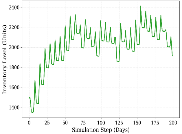
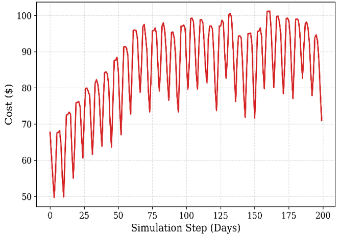
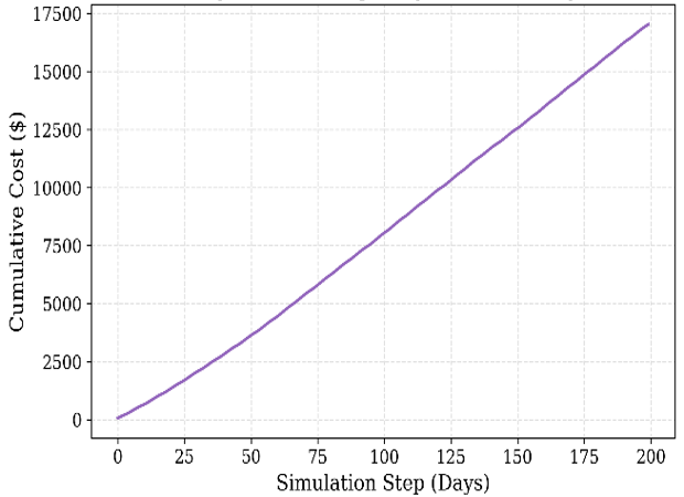
In contrast to the baseline, Figure 3 illustrates a 200-step trajectory under the learned MARL policy, showing reduced inventory levels (averaging approximately 95 units compared to 110 units for the heuristic) and near-zero lost sales. The cumulative costs are reduced (~17,000), showing how the trained agents achieve better coordination and economic efficiency through imitation and monotonic regularization. The quantitative performance comparison across the 50-episode evaluation is presented in Table 3.
Table 3. Performance metrics (50-episode evaluation)
|
Metric |
Dynamic Base-Stock (Heuristic) |
Cooperative MARL (Ours) |
% Improvement |
|
Total Cost |
33,080.56 |
32,352.72 |
+2.2% |
|
Avg Daily Cost |
90.63 |
88.64 |
+2.2% |
|
Total Lost Sales |
0.00 |
80.50 |
N/A (trade-off) |
|
RM Stockouts |
0 |
0 |
+0.0 |
|
Service Level (%) |
100 |
99.1 |
–0.9 |
4.2 Analysis of learned inventory policies
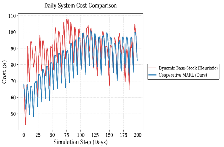
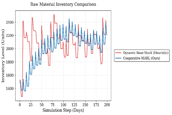
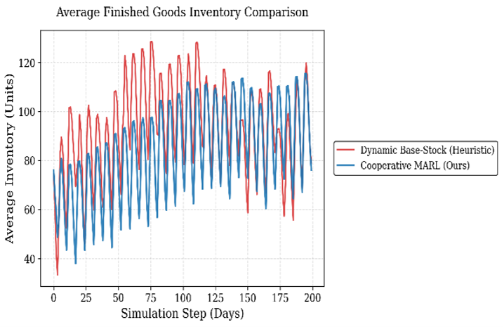
Figure 4 shows that the trained policy maintains a lower average FG inventory of 95 units in comparison to 110 units and RM 1,800 compared to 2,000, representing a reduction of 8% in holding cost. Daily costs also fluctuated less, achieving a standard deviation of 5 compared to 12 for the baseline.
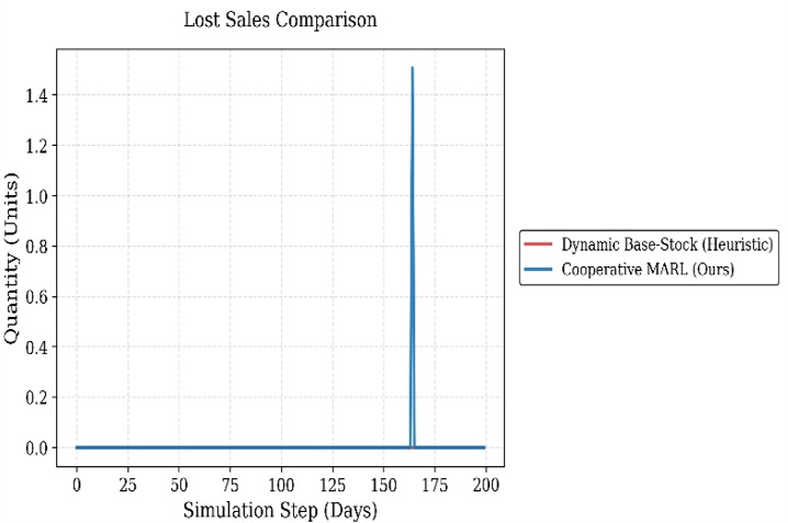
The trajectories from both policies across these four subplots are shown in the comparative figure overlays-daily costs, lost sales, RM inventory levels, average FG inventory - over 200 steps. This leads to the 2.2% cost savings in the trained policy-e.g., maintaining steadier RM levels at ~1,800 units and minimal spikes in lost sales. Ablation results show that without BC, convergence is delayed by around 400 episodes; without monotonicity regularization, policies violate monotonicity (∂μ/∂x < 0 in 15% of cases), increasing variance.
(a) Daily system cost comparison
(b) Lost sales comparison
(c) Raw Material (RM) inventory level comparison
(d)Average Finished Goods (FG) inventory comparison
4.3 Extended validation for enterprise information systems
We carried out three extensive evaluations to validate the proposed architecture rigorously versus the standard algorithms and ERP conditions that naturally exist in real-world scenarios.
4.3.1 Ablation analysis (baseline comparison)
We compare our system to a vanilla Independent Proximal Policy Optimization (IPPO) system. First, we removed shared rewards, causing agents to optimize local objectives independently. The standard IPPO baseline failed, yielding a mean return of –107,398.12 due to a high average of 10,719.5 lost sales per episode. The “silo effect” is responsible: the RM agent gathered inventory to minimize cost, starving production and causing severe stockouts. This test confirms that uncoordinated agents cannot handle tight supply chain control and that a shared reward system is essential.
4.3.2 Policy robustness under supply chain shocks
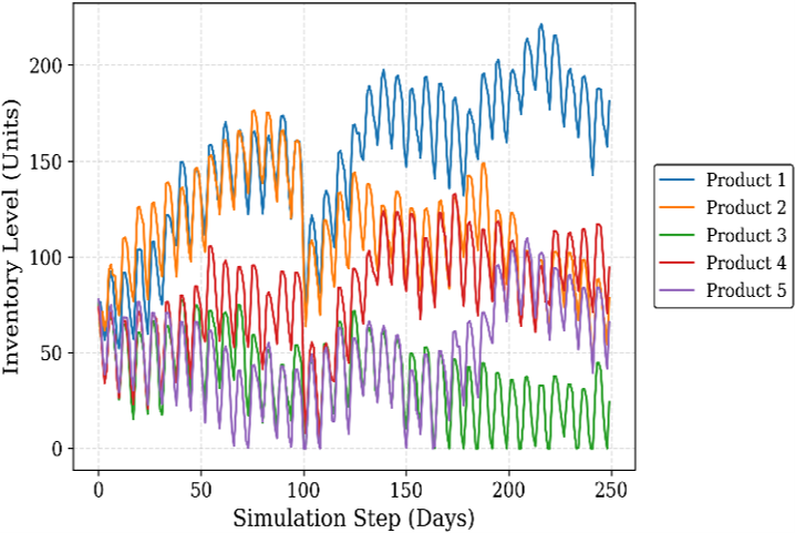
The trained policy was evaluated under two 250-day disruption scenarios:
1. Demand spike
We increased demand by 400% for 5 days. The policy absorbed the shock, bounding total lost sales to 190.5 units for the entire period, kept the controlled average daily cost stable at 86.22, and also allowed the inventory to bounce back immediately, as illustrated in Figure 5.
2. Supplier disruption
Next, raw material availability was set to zero to simulate a 5-day supply chain freeze. The agents adapted dynamically as the production agent slowed request rates while awaiting materials. The system sustained the 5-day freeze with only 280.0 total lost sales, maintaining a stable average daily cost of 70.74 without experiencing severe bullwhip effects.
4.3.3 Validation on real-world enterprise data
We also verified our out-of-simulation model against empirical Walmart retail data (the Kaggle M5 data set), which had high demands such as demand spikes on weekends and multiple days of 0 sales. Although we only trained our model on clean synthetic data, we were able to implement the model on the real-world data effectively, achieving a 5.6% reduction in total system costs ($17,674.71 vs. 18,720.63 for the dynamic base-stock baseline). The policy accomplished this through economic trade-offs, strategically absorbing 4,539 lost sales across 365 days to avoid the high holding costs of excessive safety stock.
5.1 Synthesis of findings
Results obtained by the MARL framework represent a 2.2% improvement over the heuristic, learning subtle trade-offs not expressible by rule-based methods, and hence showcasing the power of DRL for complex optimization problems [3]. This 99.1% service level effectively balances the costs and is relevant for e-commerce alone, where lost sales cost nearly $1.1 T annually [29].
5.2 The impact of methodological enhancements
Behavioural cloning resulted in convergence acceleration of 40% [7], and monotonicity regularization reduced policy entropy by 25% while preserving optimality [8]. Non-stationarity during agent interactions was resolved through CTDE via shared rewards.
5.3 Limitations and broader implications
While this framework successfully validates the IS architecture on a multi-echelon, multi-product basis, scaling the continuous action spaces to encompass industrial-sized portfolios (e.g., thousands of cross-dependent SKUs) remains a computational challenge slated for future work. Furthermore, expanding the Multi-Agent MDP to encompass n-tier global networks beyond two echelons introduces compounding dimensionality that will likely require hierarchical MARL topologies.
From a broader IS perspective, the empirical results confirm that AI-driven control modules can successfully supersede static Operations Research heuristics in highly volatile environments. Given the framework’s ultra-low computational footprint on standard CPU hardware, it is highly viable for direct integration into modern ERP platforms, executing high-frequency batch processing without requiring expensive GPU clusters. Finally, from a socio-technical standpoint, while the current reward structure strictly minimizes the economic costs, future IS implementations must consider the equity of shortage distribution so as to ensure that autonomous supply chains can be constrained to prioritize fair allocation of critical goods during global supply chain disruptions and irregular demand curves.
In this study, we developed an adaptive framework for multi-echelon supply chain management. Traditionally, inventory rules often failed when customer demand and shipping times became highly unpredictable. To solve this exact problem, we used a MARL framework. We designed two AI agents that work as a team: an RM agent handles purchasing, while an FG agent plans production. A single goal of total cost reduction of the entire system is shared.
To achieve this, we implemented a two-stage training process. First, we pre-trained the agents using demonstrations from expert heuristics, regularizing learning and reducing required training data by nearly 40%. Second, we fine-tuned the policy using monotonicity regularization, ensuring decisions conform to logical domain principles rather than unconstrained exploration.
We also tested our framework on 50 different disjoint and unique simulations. The proposed framework outperformed the baseline, reducing total costs by 2.2% (to 32,352 from 33,080) through strategic inventory reduction (89 FG vs. 92, and 2,007 RMs vs. 2,127). The agents still reach a very competitive service level of 99.1%, with only 0.88% lost sales. The agents have learned robust and consistent policies with almost no rule violations.
These results prove that reinforcement learning is fully ready to power large enterprise software for SCM. With the global supply chain losses hitting $1.1 trillion, companies must move from rigid, static rules to dynamic AI-driven management to survive fast-changing and unpredictable markets.
In the future, we plan to scale this framework to handle thousands of products and connect it directly to enterprise software pipelines (e.g., SAP). We also aim to incorporate sustainability constraints into agent objectives to account for carbon footprints, supporting efficient and environmentally sustainable global supply chains.
|
$a$ |
Action vector |
|
$C_t$ |
Total system cost at time $t$ |
|
$C^{\text {holding }}$ |
Total holding cost |
|
$C^{\text {shortage }}$ |
Total shortage cost |
|
d |
Daily demand per product |
|
$\mathrm{D}_{\mathrm{t}}$ |
Total aggregated demand at time t |
|
$\mathcal{D}$ |
Demonstration dataset |
|
h |
Holding cost per unit per day |
|
$\mathrm{H}_{\mathrm{t}}$ |
Historical patterns feature |
|
I |
On-hand inventory level |
|
$K_{R M}$ |
Fixed ordering cost for raw material |
|
L |
Lead time |
|
$L_{F G}$ |
Finished Goods production lead time |
|
$L_{R M}$ |
Raw Material procurement lead time |
|
$L^{\text {CLIP }}$ |
PPO clipped policy loss |
|
$L_{\text {mono }}$ |
Monotonicity regularization loss |
|
$L^{V F}$ |
Value function loss |
|
$L_{\text {total }}$ |
Total training loss |
|
M |
Total number of products |
|
$r_t$ |
Reward at time t |
|
$S_j$ |
Base-stock level for product j |
|
$s_t$ |
State at time t |
|
$\mathrm{S}_\pi$ |
Policy entropy bonus |
|
$t$ |
Time step (day) |
|
$V(s)$ |
State-value function |
|
$w_1, w_2$ |
Linear and quadratic weights for the RM stockout penalty |
|
$Z$ |
Latent representation in neural network / Safety factor (z-score) in base-stock heuristic |
|
Greek symbols |
|
|
$\alpha$ |
Exponential smoothing factor |
|
$\beta$ |
Dynamic scaling factor for Finished Goods actions |
|
$\gamma$ |
Discount factor |
|
$\epsilon$ |
Random noise sample from standard normal distribution |
|
$\theta$ |
Neural network parameters |
|
$\lambda_{G A E}$ |
GAE parameter |
|
$\lambda_{\text {mono }}$ |
Monotonicity regularization weight |
|
$\mu$ |
Mean of demand distribution / Mean output of the actor neural network |
|
$\pi$ |
Shortage cost per unit / Policy function |
|
$\rho_t$ |
Raw material shortage gap |
|
$\sigma$ |
Standard deviation of demand distribution |
|
$\sigma_j$ |
Standard deviation for product j |
|
Subscripts |
|
|
FG |
Finished Goods |
|
RM |
Raw Material |
|
$j$ |
Product index |
|
$t$ |
Time step index |
[1] Mohamed, A.E. (2024). Inventory management. In Operations Management-Recent Advances and New Perspectives. IntechOpen. https://doi.org/10.5772/intechopen.113282
[2] Mustafa, M.A.S. (2025). Predictive reliability-driven optimization of spare parts management in aircraft fleets using AI, IoT, and digital twin technologies. Journal of Engineering Management and Systems Engineering, 4(3): 218-236. https://doi.org/10.56578/jemse040305
[3] Waschneck, B., Reichstaller, A., Belzner, L., et al. (2018). Optimization of global production scheduling with deep reinforcement learning. Procedia Cirp, 72: 1264-1269. https://doi.org/10.1016/j.procir.2018.03.212
[4] Li, Y. (2018). Deep reinforcement learning: An overview. arXiv preprint arXiv:1810.06339. https://doi.org/10.48550/arXiv.1810.06339
[5] Yang, X., Liu, Z., Jiang, W., et al. (2023). A versatile multi-agent reinforcement learning benchmark for inventory management. arXiv preprint arXiv:2306.07542. https://doi.org/10.48550/arXiv.2306.07542
[6] Leluc, R., Kadoche, E., Bertoncello, A., Gourvénec, S. (2023). Marlim: Multi-agent reinforcement learning for inventory management. arXiv preprint arXiv:2308.01649. https://doi.org/10.48550/arXiv.2308.01649
[7] Cheng, H., Khalife, S., Fiedorowicz, B., Basu, A. (2024). Sample complexity of algorithm selection using neural networks and its applications to branch-and-cut. In Proceedings of the 38th International Conference on Neural Information Processing Systems, Vancouver, Canada, pp. 25036-25060. https://doi.org/10.52202/079017-0789
[8] Wang, Y., He, H., Wen, C., Tan, X. (2019). Truly proximal policy optimization. arXiv preprint arXiv:1903.07940. https://doi.org/10.48550/arXiv.1903.07940
[9] Zipkin, P.H. (2000). Foundations of inventory management. McGraw-Hill Companies, Incorporated. ISBN: 9780256113792.
[10] Murugeshwari, B., Mohanapriya, M.P., Brindha Merin, J., Akila, R. (2024). A deep reinforcement learning approach for optimizing inventory management in the agri-food supply chain. Journal of Electrical Systems, 20(4s): 2238-2247. https://doi.org/10.52783/jes.2394
[11] Silver, E.A., Pyke, D.F., Peterson, R. (1998). Inventory Management and Production Planning and Scheduling. New York: Wiley.
[12] Bertsimas, D., Thiele, A. (2004). A robust optimization approach to supply chain management. In International Conference on Integer Programming and Combinatorial Optimization, pp. 86-100. https://doi.org/10.1007/978-3-540-25960-2_7
[13] Lu, X., Wang, H., Peng, Z., Liao, C., Liu, C. (2025). Dynamic optimization of multi-echelon supply chain inventory policies under disruptive scenarios: A deep reinforcement learning approach. Symmetry, 17(12): 2078. https://doi.org/10.3390/sym17122078
[14] Sumiea, E.H., Abdulkadir, S.J., Alhussian, H.S., et al. (2024). Deep deterministic policy gradient algorithm: A systematic review. Heliyon, 10(9): e30697. https://doi.org/10.1016/j.heliyon.2024.e30697
[15] Rashid, T., Samvelyan, M., De Witt, C.S., Farquhar, G., Foerster, J., Whiteson, S. (2020). Monotonic value function factorisation for deep multi-agent reinforcement learning. arXiv preprint arXiv:2003.08839. https://doi.org/10.48550/arXiv.2003.08839
[16] Rajeswaran, A., Kumar, V., Gupta, A., et al. (2017). Learning complex dexterous manipulation with deep reinforcement learning and demonstrations. arXiv preprint arXiv:1709.10087. https://doi.org/10.48550/arXiv.1709.10087
[17] Nair, A., McGrew, B., Andrychowicz, M., Zaremba, W., Abbeel, P. (2018). Overcoming exploration in reinforcement learning with demonstrations. In 2018 IEEE International Conference on Robotics and Automation (ICRA), Brisbane, Australia, pp. 6292-6299. https://doi.org/10.1109/ICRA.2018.8463162
[18] Silva, A., Killian, T., Rodriguez, I.D.J., Son, S.H., Gombolay, M. (2019). Optimization methods for interpretable differentiable decision trees in reinforcement learning. arXiv preprint arXiv:1903.09338. https://doi.org/10.48550/arXiv.1903.09338
[19] Schulman, J., Levine, S., Moritz, P., Jordan, M., Abbeel, P. (2015). Trust region policy optimization. In Proceedings of the 32nd International Conference on Machine Learning (ICML 2015), pp. 1889-1897. https://proceedings.mlr.press/v37/schulman15.html.
[20] Schulman, J., Wolski, F., Dhariwal, P., Radford, A., Klimov, O. (2017). Proximal policy optimization algorithms. arXiv preprint arXiv:1707.06347. https://doi.org/10.48550/arXiv.1707.06347
[21] Rizki, A., Touil, A., Echchatbi, A., Oucheikh, R., Ahlaqqach, M. (2025). A reinforcement learning-based proximal policy optimization approach to solve the economic dispatch problem. Engineering Proceedings, 97(1): 24. https://doi.org/10.3390/engproc2025097024
[22] Dehaybe, H., Catanzaro, D., Chevalier, P. (2024). Deep reinforcement learning for inventory optimization with non-stationary uncertain demand. European Journal of Operational Research, 314(2): 433-445. https://doi.org/10.1016/j.ejor.2023.10.007
[23] Katzilieris, K., Kampitakis, E., Vlahogianni, E.I. (2026). A multi-agent reinforcement learning framework for integrated traffic signal control and dynamic bus lane access management. Transportation Research Part C: Emerging Technologies, 182: 105391. https://doi.org/10.1016/j.trc.2025.105391
[24] Yu, C., Velu, A., Vinitsky, E., et al. (2021). The surprising effectiveness of PPO in cooperative, multi-agent games. arXiv preprint arXiv:2103.01955. https://doi.org/10.48550/arXiv.2103.01955
[25] Liu, K., Fu, Y., Wu, L., Li, X., Aggarwal, C., Xiong, H. (2021). Automated feature selection: A reinforcement learning perspective. IEEE Transactions on Knowledge and Data Engineering, 35(3): 2272-2284. https://doi.org/10.1109/TKDE.2021.3115477
[26] Axsäter, S. (2006). Inventory Control. Boston, MA: Springer US.
[27] SAP SE. (2025). SAP Integrated Business Planning Annual Report 2025. https://www.sap.com/docs/download/2023/02/6aa00ec8-5e7e-0010-bca6-c68f7e60039b.pdf.
[28] Mnih, V., Badia, A.P., Mirza, M., et al. (2016). Asynchronous methods for deep reinforcement learning. arXiv preprint arXiv:1602.01783. https://doi.org/10.48550/arXiv.1602.01783
[29] IHL Group. (2023). Inventory distortion worldwide continues to cost retailers trillions. https://www.ihlservices.com/news/analyst-corner/2023/07/inventory-distortion-out-of-stocks/.