Asmaa Hussein Alwan | Nuha Sami Mohsin* | Abdullah Hasan Ali
© 2026 The authors. This article is published by IIETA and is licensed under the CC BY 4.0 license (http://creativecommons.org/licenses/by/4.0/).
OPEN ACCESS
Quantum annealing (QA) has attracted increasing attention for solving complex combinatorial optimization problems, but its practical application remains limited by hardware constraints, including embedding overhead, chain breaks, and noise-induced degradation. This study proposes an Adaptive Hybrid Quantum Annealing (AHQA) framework that integrates an adaptive nonlinear annealing schedule, an energy-weighted dynamic chain repair mechanism, and a unified evaluation metric named the Quantum Advantage Ratio (QAR). The proposed scheduling strategy introduces adaptive pausing according to energy evolution characteristics, while the chain repair method improves logical solution consistency by incorporating energy information from multiple samples. The framework is evaluated on three representative Operations Research (OR) problems: Vehicle Routing Problem (VRP), Portfolio Optimization, and Job Shop Scheduling (JSS), using the D-Wave Advantage quantum processor and classical optimization baselines. Experimental results show that AHQA improves approximation quality and reduces Time-to-Solution (TTS) compared with conventional QA approaches. The proposed chain repair mechanism decreases chain break rates, while QAR provides a unified perspective for comparing solution quality and computational efficiency. The results indicate that the effectiveness of QA is strongly influenced by problem structure, particularly connectivity density and embedding complexity. This study demonstrates a practical hybrid quantum-classical strategy for current quantum hardware and provides insights into the application of QA in logistics, financial optimization, and manufacturing scheduling.
quantum annealing, hybrid quantum-classical optimization, adaptive scheduling, dynamic chain repair, quadratic unconstrained binary optimization, combinatorial optimization, Quantum Advantage Ratio
Optimization and the use of mathematical models and algorithms to minimize complexity in systems such as logistics, finances, manufacturing, and other industrial fields have been integral to Operations Research (OR) as a decision-making tool for decades. Conventional optimization methods, such as linear programming, branch and bound, and heuristic methods such as simulated annealing [1], are used to optimize problems ranging from the design of a supply chain to optimizing a portfolio. However, most combinatorial and continuous optimization problems, particularly Non-deterministic Polynomial-time hard (NP-hard) ones such as the Quadratic Assignment Problem (QAP) and the Traveling Salesman Problem (TSP), have computational complexity of exponential size [2] and cause scalability challenges. Classical solvers are now bogged down in undecidable runtime or do not lead to optimal solutions in the face of increasingly complex and large challenges [3].
One of the technologies now seeing great potential to transform the boundaries of computational optimization is quantum computing. Optimization problems are one of the many types of problems that quantum annealing (QA) is well suited for. Unlike traditional thermal annealing techniques, QA can be used to better traverse the landscape of solutions using quantum mechanical processes, including quantum tunneling and entanglement [4]. Compared with gate-based quantum computing, which applies discrete processes, a quantum adiabatic computer (QA) functions by gradually changing a quantum system from an initial Hamiltonian to a problem Hamiltonian that represents the optimization objective [5]. This technique is especially suitable for problems formulated as Ising spin glass models or quadratic unconstrained binary optimization (QUBO) problems commonly encountered in OR [6]. Recent advances, such as D-Wave's Advantage platform, have increased the number of qubits that can be interconnected, and scalability has improved [7], which makes issues with more than 5,000 variables soluble.
Despite these theoretical hopes and equipment improvements, the use of QA on a larger scale for OR problems is still a subject of debate. Despite many studies demonstrating speedups for certain classes of problems, e.g., Job Shop Scheduling (JSS) and vehicle routing [8], these speedups are typically constrained by significant physical limitations including environmental noise, limited availability of qubits, and qubit decoherence. Furthermore, the translation of real-world OR problems to QUBO/Ising formulation requires more complexity and careful tuning of parameters [9]. While in some cases QA can outperform traditional solvers, especially in problems with non-convex or multimodal energy landscapes, the study [10] has demonstrated that dense problem graphs are a challenge for QA due to the high embedding overhead. As examples, FedEx has conducted tests for last-mile delivery routing with QA, and Volkswagen AG has explored QA for optimising traffic flow in urban settings for small-to-medium-sized examples, with competitive Time-to-Solution (TTS). These applications are found in the logistics industry. Similarly, Siemens has experimented with scheduling power grids using QA, and it has been used in finance to optimize portfolios with near-optimal allocations achieved for portfolios comprising over 100 assets at JP Morgan Chase. Along with those industrial pilots, there is an increased interest in quantum-assisted optimization with the awareness that there is a difference between what can be achieved in the laboratory and what will be deployed in operational systems.
This study fills several holes in the literature. Without offering a coherent methodology that methodically addresses issues relating to algorithms and hardware, earlier research has concentrated on either theoretical formulation for quality assurance problems or hardware benchmarking, limiting itself to specific aspects of quality assurance performance. Second, because the types of evaluation measures employed in the various studies are not consistent, it is difficult to compare their performance and be confident in the real benefits of QA. Among the notable obstacles to scalability, thirdly, are the lack of adaptive methods that effectively address hardware constraints, including hardware shimming and hardware embedding inefficiencies. Finally, there is not enough discussion of the use of quality control in the real world, and there are no standardized benchmarking methods, which has prevented the inclusion of quality control into operational decision-making processes.
This work proposes an Adaptive Hybrid Quantum Annealing (AHQA) Framework with three novel contributions to bridge these gaps: (i) a novel non-linear annealing schedule with adaptive pausing for better explorative performance than classical counterpart linear scheduling and significantly improved exploitation performance; (ii) an energy-weighted dynamic chain repair mechanism that significantly reduces the effects of broken chain qubits by combining knowledge over many different samples to achieve high logical solution validity; and (iii) a novel performance measure: Quantum Advantage Ratio (QAR), proposed to quantify the practical speedup and quality gain of the QA method over classical state-of-the-art methods. Unlike prior research that employed synthetic benchmarks, we confirm our framework with a comprehensive set of experiments on D-Wave's Advantage quantum processor using three representative OR problem classes: the JSS, Portfolio Optimization, and Vehicle Routing Problem (VRP).
Because it is the most developed and commercially available platform for QA-based optimization, this study is restricted to D-Wave quantum annealers. Alternative quantum paradigms, such as gate-based ones like VQE and QAOA, which are not applicable to large-scale OR problems, are not considered here. Moreover, the proposed framework, even if tested for three OR problem classes, should be investigated for other problem classes like the quadratic assignment or facility location problem classes. Other trade-offs may be made using other heuristics; the main classical baselines used are CPLEX, Gurobi, and simulated annealing.
This study has ramifications outside of academia and may be utilized as a guide for businesses that want to experience the quantum edge in areas like financial risk management, smart manufacturing, and logistics optimization. The study provides insights into the development of algorithms that combine quantum and classical methods and future hardware for scalable optimization using quantum computers, thereby helping to close the gap between theory and practice in OR. The proposed AHQA framework not only outlines a viable approach to quantum-assisted decision making, but also identifies key hardware and algorithm development needs to make quantum computing a viable technology for industrial-scale optimization.
This part contains a detailed discussion of fundamental concepts, mathematical models, hardware architectures, performance restrictions, and the field of application for QA in the field of OR. The assessment is organized to methodically pinpoint the holes in the current literature that prompt the suggested AHQA. This section critically examines the state of the art and identifies the similarities and differences between the known techniques and the newer ones, as well as identifying special hardware limitations that are not addressed by previous techniques.
2.1 Applying the theory of quantum annealing for solving optimization problems
This is the theoretical underpinning of QA, which is based on the quantum mechanical adiabatic theorem. This study [11] had the idea of adiabatic quantum computation, in which a quantum system initially placed in the ground state of a Hamiltonian would remain there if the Hamiltonian could be evolved slowly enough into a different Hamiltonian whose ground state would be the solution to the optimization problem. This is mathematically ensured by adiabatic progression, which makes the system converge to the optimum global solution for an infinite time.
But realistically, a finite annealing time produces a diabatic transition, which drives the system from the ground state, leading to suboptimal solutions [12]. A big challenge in QA research remains to strike the right balance between the quality of the solution and the duration of the annealing process. From theoretical studies, it is believed that longer annealing times achieve better quality of the solution; however, from empirical studies, it is found that, after a certain point, the relation between the time and the quality of the solution is not linear, and further increases in the annealing time led to diminishing returns due to decoherence and accumulation of noise [13]. This has led to the research of more complex and sophisticated annealing schedules which balance the exploration/exploitation components more effectively than linear schedules. Many of the mathematical formulations for QA issues involve the Ising model or some equivalent such as the QUBO framework. The Ising Hamiltonian is represented as:
$H=\sum_{i<j} J_{i j} \sigma_i^z \sigma_j^z+\sum_i h_i \sigma_i^z$
where, $J_{i j}$ represents the interaction strength between spins $i$ and $j, h_i$ denotes the local magnetic field, and $\sigma_i^z$ are Pauli-Z operators acting on spin $i$ [14]. The QUBO formulation, which is mathematically equivalent through a simple variable transformation $x_i=\left(1+\sigma_i^z\right) / 2$, expressed as:
$\min _{\mathbf{x} \in\{0,1\}^n} \mathbf{x}^T Q \mathbf{x}$ (1)
where, Q is an $n \times n$ upper-triangular matrix of coefficients [15]. Both formulations are widely used in OR applications due to their ability to represent a broad class of combinatorial optimization problems.
2.2 Hardware structures and topological limits
D-Wave Systems has been the top commercial vendor of QA devices with successive generations that have steadily increased the number of qubits and connectivity. The Chimera topology of the D-Wave 2000Q processor limited its connectivity: Each qubit could only connect to four or five others. A Pegasus topology with up to 15 neighbors for each qubit was realized using the D-Wave Advantage platform. This made it much easier to establish connections and to solve problems with over 5,000 variables [16]. Although extensive benchmarking data is still being released [17], the newest Zephyr topology provides even better connectivity.
In practice, the physical connectivity graph of the quantum processor often differs from the logical connectivity graph required for real-world OR problems. However, this difference demonstrates the need to link logical qubits onto a chain of physical qubits. A thorough study indicates that the embedding overhead is the most important factor to determine scalability and performance; greater qubit count alone is not relevant [18]. For thick problem graphs, the capacity of a real problem may be reduced by 80–92% with each logical variable requiring 5 to 12 physical qubits [19]. This severe reduction in qubit efficiency ($\eta=N_{\text {logical}}/N_{\text {physical}}$) fundamentally limits the size of problems that can be practically solved on current hardware.
2.3 Chain break and embedding overhead
There are two critical problems with embedding: chain breaks and parameter scaling. If the actual qubits on the chain are not all stabilized in the same end state, then chain breaks occur, leading to logical solutions that are incorrect. Chain breaks increase with the length of the chain, as well as any error caused by imperfections in the chain and any errors caused by noise [20]. Empirical studies have shown that the chain break rate ranges from 10% for sparse issues up to more than 25% for dense problem situations [21].
Recent work [22] has developed closed-form equations for the probability of chain breakage for several noise models that are Gaussian with embedding-aware error signals. These models suggest a critical compromise: While the strength of the chain can be increased (that is, increase the coupling between the qubits in a chain), the chain becomes less useful by altering the system away from the true best answer. The optimum chain strength will vary with the problem, and it is normally necessary to employ “empirical tuning”. The study [23] has shown that there is no linear relationship between the validity of the solution and chain break rates. These post-processing methods are not sufficient to find valid solutions if the number of chain breaks is more than around 20%.
The impact of embedding overheads is not limited to areas of chain breaks. The relaxation dynamics and annealing itself are also altered by the presence of chains; longer chains have slower relaxation dynamics and for higher sensitivity to noise. According to research, embedding adds additional complexity to the optimization landscape since the energy variance of sampled solutions increases substantially with chain length [24]. It underscores the need for adaptive embedding methods, considering problem structure and hardware constraints.
2.4 Optimizing the annealing schedule
The key role in determining the performance of the QA is played by the annealing schedule, i.e., the time evolution of the system Hamiltonian. The time-dependent Hamiltonian is given by:
$H(t)=A(t)\left(-\sum_i \sigma_i^x\right)+B(t)\left(\sum_{i<j} J_{i j} \sigma_i^z \sigma_j^z+\sum_i h_i \sigma_i^z\right)$ (2)
where, $A(t)$ controls the transverse field (driver Hamiltonian) and $B(t)$ controls the problem Hamiltonian. In standard linear schedules, $A(t)=1-t / \tau$ and $B(t)=t / \tau$, where $\tau$ is the total annealing time. However, recent research has demonstrated that non-linear schedules with pausing can significantly improve performance [25].
Pausing is to hold a constant intermediate annealing parameter in the schedule to let the quantum system relax at this point before continuing the evolution. Empirical studies indicate that for some problems the odds of success are significantly increased when pausing [26]. It is believed that appropriate intervention in time helps prevent diabatic transitions and promotes quantum tunneling, resulting in better performance in the stopping of the quantum. But another open research question in the literature exists [27] concerning the best place and time for a pause, which are problem-dependent.
Apart from pausing, several more elaborate schedules have been explored, such as reverse annealing (beginning at the problem Hamiltonian and going back), multi-stage schedules with multiple pauses, and adaptive schedules that react to the real-time measurements of the quantum state [28]. Despite these advances, there is no universal method to systematically optimize the schedule of annealing for different classes of problems and hardware configurations.
2.5 Quantum-classical hybrids
QA in combination with classical computation has been developed as a practical way forward for real-world applications in view of the constraints imposed by current quantum hardware. Hybrid workflows have been developed by D-Wave; they split problems into chunks that are worked on by classical and quantum processors, allowing for still more practical applications [29]. Their hybrid solvers further increase the range of relevant OR areas, e.g., production planning and supply chain management, by solving mixed integer linear programming (MILP) problems.
Top classical solvers, like CPLEX, Gurobi, and IPOPT, have been evaluated against D-Wave’s hybrid solvers in benchmark studies. The latest result is that the hybrid solver should be the best choice for sparse constrained integer quadratic objective functions [30]. For nearly linear limits or dense problems, classical solvers are typically better. This result indicates that it is important to select algorithms based on the problem at hand, as opposed to viewing QA as a one-size-fits-all replacement for traditional methods.
Novel and pioneering hybrid approaches have been proposed in the literature. Learning Machine (LM) [31] achieves a machine-learning-enhanced parameter optimization over multiple iterations, linking consecutive QA runs to a global solution framework in addition to single QA evolutions. It has been established that iterative cyclic QA algorithms can also quickly locate deep low-energy states on gigantic spin glasses [32]. These approaches lend themselves to the inclusion of co-design between classical and quantum parts of a system, though they also expose the lack of well-defined methodologies for hybrid algorithm design and development.
2.6 Metrics for evaluation and performance benchmarking
A broad range of research has been dedicated to the methodical comparison of quantum annealers with traditional solvers. McGeoch and colleagues conducted an in-depth evaluation of QA in relation to simulated annealing and CPLEX for traveling salesman and graph partitioning challenges. Their findings revealed that QA exhibited a competitive TTS for problems involving up to 100 variables, yet its performance was hindered with larger problems due to overhead associated with embedding [33]. The study [34] looked at hardware performance via control error and noise on qubit fidelity and its impact on solution quality for different generations of D-Wave systems.
One of the main problems is the differences in the measures adopted to assess the selected studies. This is usually the case, and TTS is calculated based on the target success probability (p) and the probability of success during each anneal (f), the latter of which is often approximated in various manners in different studies. The approximation ratio (ρ) is a normalized measure of solution quality and assumes that the true optimal solution is known, which affects interpretation. Also, chain breaks and noise are not taken into account for qubit efficiency (η), which uses embedding overhead.
To overcome the lack of consistency, the researchers suggest standard instance generators and new benchmarking procedures. There have been recent advances towards the construction of graph instances that have near-optimal minor-embedding mappings which can be used to make more meaningful performance comparisons [35, 36]. But there is a very significant gap, since the usefulness of QA as a tool to traditional approaches cannot be fully quantified by a single number. To close this gap, the QAR, motivated by this study, aims at capturing both the speed-up and quality aspects in a single easy-to-interpret measure.
2.7 Applications in Operations Research
•VRP: QA has been extensively applied to VRPs, which play a fundamental role in logistics optimization. We demonstrate the process of mapping integer programming models to QUBO problems, which can be solved using the D-Wave Advantage quantum computer [37]. They report devices being configured by several applications of this kind, which exhibit approximation ratios in the interval from 0.82 to 0.88. Tight time window constraints allowed for a maximum of 50 delivery nodes and time window constraints. However, the quaternarization of QUBO variables may scale up with the number of nodes; the expansion makes it challenging to address larger problems.
•Portfolio Optimization: QA is widely used in financial terms for Portfolio Optimization. In mean-variance optimization, the quadratic objective functions can be directly incorporated in the QUBO formulation [38]. In some market situations, near-optimal allocations for portfolios, including more than 100 assets, are reported to achieve approximation ratios beyond 0.90. However, the performance of QA is heavily dependent on the structure of the covariance matrix and on the choice of penalty parameters for constraints, and even a slight change can cause a significant difference.
•JSS: Since scheduling problems are both NP-hard and important to industry, they have attracted a lot of study. There has been an investigation on how some types of scheduling problems can be transformed into QUBO models suitable for current quantum devices [39-44]. On the other hand, the solution quality is weakened by more than 20% broken chains, and such results are prone to being invalid. The high connectivity requirements of scheduling problems exacerbate embedding overhead [45-50], and so scalability is limited by the latter factor as well.
•Other applications. Beyond these basic OR problems, the Max-Cut problem, graph partitioning and community detection in complex networks [51-54], seismic inverse analysis [55], and power grid optimization [56] represent other applications of QA. Common problems that arise in many application domains, such as embedding, noise, and scalability, are highlighted by these diverse applications, but they also show the flexibility of the QUBO formulation.
2.8 Gaps in the research
This is a detailed analysis of five important gaps that together drive the AHQA model that is suggested in this work:
Prior work has studied individual components of the QA performance, ranging from hardware-level benchmarking to theoretical formulation of a QUBO to application-specific studies, but not at the integrated level where the algorithmic- and hardware-level components are all considered. There is no universal method that would simultaneously optimize annealing schedules, prevent chain failures, and provide a complete performance evaluation.
Current schedule optimization and embedding methods are mostly static and are not aware of specific problem features or real-time hardware conditions. The lack of adaptive methods that respond to detected chain breaks, different noise levels, or energy landscape features is a significant limitation:
•Discrepancies and gaps in metrics: Benchmarks can be problematic as the metrics used for evaluation differ among studies, making direct performance comparisons difficult. In addition, no measure so far completely captures the functional advantage that QA has over classical methods. The proposed QAR measure can fill this gap.
•No industrial validation: There are industrial pilots, but little discussion of benchmarking the standards and guidelines for real deployment. There is still a big gap between full-scale system implementation and laboratory demonstration.
•Schedule gap optimization: While pausing has been shown to be effective, research on adaptively optimizing non-linear schedules is still scarce.
The motivated contributions of this paper are: an energy-weighted dynamic chain repair method; the QAR as a comprehensive performance measure; and a novel adaptive pausing, dynamically optimized non-linear annealing schedule. The AHQA framework straddles these gaps in one framework, combining theory and practice and offering practical examples of how to apply QA in practical OR cases.
The AHQA is presented in this section following a full description of the methodology of this work. The presentation consists of two separate parts: (A) Standard Building Blocks (Sections 3.1–3.4), which defines the baseline QUBO formulations and experimental setting, and (B) Our Novel Contributions (Sections 3.5–3.6), where the three novel contributions of this work are presented.
3.1 Standard components
3.1.1 Quadratic unconstrained binary optimization formulation for Operations Research problems
The QUBO formulation is the common ground for quantum annealers. Given an optimization problem with binary decision variables $x \in\{0,1\}^n$, the objective is expressed as a quadratic pseudo-Boolean function:
$\begin{gathered}\min _{\mathbf{x} \in\{0,1\}^n} f(\mathbf{x})=\min \left(\sum_i Q_{i i} x_i+\sum_{i<j} Q_{i j} x_i x_j\right) =\min \mathbf{x}^T Q \mathbf{x}\end{gathered}$ (3)
where, Q is an $n \times n$ upper-triangular matrix. For constrained problems, equality constraints $A \mathbf{x}=b$ are incorporated using the quadratic penalty method, yielding the penalized objective:
$\min _{\mathbf{x}}\left(\mathbf{x}^T Q \mathbf{x}+\lambda \sum_k\left(A_k \mathbf{x}-b_k\right)^2\right)$ (4)
Following standard practice, we set $\lambda=10 \times\|Q\|_2$ to ensure feasibility, consistent with the recommendations in the study by Hao et al. [41]. This penalty parameter is validated through sensitivity analysis across all problem classes.
3.1.2 Problem-specific quadratic unconstrained binary optimization encodings
For the three representative OR problem classes evaluated in this study, we adopt the following standard QUBO encodings:
•VRP: For $N$ nodes and $M$ vehicles, binary variables $x_{i, j, k} \in\{0,1\}$ indicate whether vehicle $k$ traverses' edge $(i, j)$. The objective minimizes total distance with flow conservation and node-visit constraints encoded as penalties.
•Portfolio Optimization: For $N$ assets, binary variables $x_i$ indicate asset selection. The objective balances expected return $\mu_i$ against risk $\sigma_{i j}$, parameterized by risk aversion $\gamma$ : $C=-\sum_i \mu_i x_i+\gamma \sum_{i, j} \sigma_{i j} x_i x_j$ [42].
•JSS: For $J$ jobs and $M$ machines, variables $x_{j, m, t}$ indicate job $j$ on machine $m$ at time $t$. The objective minimizes makespan with precedence and resource constraints as penalties [43].
3.1.3 Illustrative conversion example: Vehicle Routing Problem to quadratic unconstrained binary optimization
We provide a concise step-by-step example of converting a small VRP instance into QUBO form.
Problem: 3 delivery nodes (A, B, C) and one depot (0). Distance matrix d is symmetric.
Step 1: Variables. Define $x_{i, j} \in\{0,1\}$ for travel from i to j. For 4 nodes, we have 12 binary variables.
Step 2: Objective. Minimize total distance:
$\min \sum_{i=0}^3 \sum_{j \neq i} d_{i, j} \cdot x_{i, j}$ (5)
Step 3: Constraints. Encode "each node visited once" $\left(\sum_{i \neq j} x_{i, j}=1\right)$ and "each node departed once" ($\sum_{j \neq i} x_{i, j}=$ 1) as squared penalties. Subtour elimination for $N=3$ is handled by explicit cycle constraints.
Step 4: Penalized form. For node A, the visit constraint penalty is:
$\lambda\left(x_{0, A}+x_{B, A}+x_{C, A}-1\right)^2$ (6)
Expanding (6) yields linear terms ($\lambda x$) and quadratic terms $\left(2 \lambda x_i x_j\right)$. Since $x_{i, j}^2=x_{i, j}$ for binary variables, all terms are naturally QUBO-compatible.
Step 5: Quadratic unconstrained binary optimization matrix construction. Collect all linear coefficients (distances + penalty contributions) on the diagonal of Q, and all quadratic coefficients on the off-diagonal. With $\lambda=10 \times \max (d)$, the resulting QUBO $\min \mathbf{x}^T Q \mathbf{x}$ is submitted to the annealer.
The optimal solution for this instance is $0 \rightarrow A \rightarrow B \rightarrow C \rightarrow$0 , with total distance 90, verified by exhaustive search. This example generalizes to larger $N$ with $N(N-1)$ variables.
3.1.4 Experimental configuration
To ensure reproducibility and confirm that results are original, we detail the experimental setup below.
•Quantum hardware: D-Wave Advantage 4.1 (Pegasus topology, 5,627 qubits, ~5,000 usable). Annealing time: 1,000–2,000 $\mu \mathrm{s}$. Reads per instance: 1,000.
•Benchmark instances: 20 VRP instances from TSPLIB (10–100 nodes); 20 portfolio instances from CRSP daily returns (20–200 assets, 2020–2024); 20 JSS instances from OR-Library (Taillard sets, 10 × 5 to 30 × 10).
•Classical baselines: CPLEX 22.1.1, Gurobi 10.0.1 (time limit 3,600s), and custom Simulated Annealing (geometric cooling).
•Implementation: Python 3.10 with D-Wave Ocean SDK 7.0. Source code and datasets are available at the anonymized repository.
3.2 Novel components of the Adaptive Hybrid Quantum Annealing framework
In this subsection, we report on the three original contributions of this study, which are clearly distinguished from the standard procedure summarized above.
3.2.1 Original contribution (i): Adaptive non-linear annealing schedule
Conventional QA employs linear schedules where $A(t)=1-t / \tau$ and $B(t)=t / \tau$.
But research related to pausing [44] indicates that non-linear evolution can greatly increase the probability of success. Based on this, we suggest a dynamically optimized non-linear schedule that includes adaptive pausing.
Our schedule features three components:
•Dynamic pause detection: Instead of a fixed pause time tp, we take an adaptive spike detection based upon the second derivative of the average sampled energy ⟨E(t)⟩ measured over a brief calibration run:
$t_p=\arg \min _{t \in[0, \tau]} \frac{d^2}{d t^2}\langle E(t)\rangle$ (7)
This is the identification of the point of maximum curvature, which is usually roughly the same as the minimum spectral gap Δmin.
•Non-linear coefficients: The schedule coefficients are defined at the point $t_p$ with a time delay of δ:
$A(t)=\left\{\begin{array}{cc}\left(1-\frac{t}{\tau}\right)^\alpha, & t<t_p \\ \left(1-\frac{t_p}{\tau}\right)^\alpha, & t_p \leq t \leq t_p+\delta \\ \left(1-\frac{t-\delta}{\tau}\right)^\alpha, & t>t_p+\delta\end{array}\right.$ (8)
$B(t)=\left\{\begin{array}{lc}\left(\frac{t}{\tau}\right)^\beta, & t<t_p \\ \left(\frac{t_p}{\tau}\right)^\beta, & t_p \leq t \leq t_p+\delta \\ \left(\frac{t-\delta}{\tau}\right)^\beta, & t>t_p+\delta\end{array}\right.$ (9)
where, $\alpha, \beta>0$ are problem-dependent exponents. For sparse problems (VRP), we set $\alpha=1.2$ to slow the initial annealing, allowing broader exploration. For dense problems (JSS), $\alpha=$ 0.8 accelerates early evolution to reduce decoherence exposure. We maintain $\beta=2-\alpha$ to approximate the adiabatic condition $A(t)+B(t) \approx 1$ outside the pause.
•Theoretical justification: The adiabatic theorem requires $\tau \gg \max _t\|[H(t), \dot{H}(t)]\| / \Delta_{\min }$ [45]. Our non-linear schedule reduces $\|\dot{H}(t)\|$ specifically around $t_p$, effectively relaxing this requirement. The pause permits the system to equilibrate at the avoided crossing, enhancing ground-state probability.
|
Algorithm 1. Energy-weighted dynamic chain repair |
|
Input: sampleset (list of (sample, energy)), chain_map (logical→physical qubits) Output: repaired_solutions (list of (logical_state, repaired_energy)) 1. E_min ← min(energies), E_max ← max(energies), E_range ← E_max - E_min 2. For each sample s in sampleset: 3. If E_range > 0: weight ← exp(-(s.energy - E_min) / E_range) 4. Else: weight ← 1.0 5. For each chain C in chain_map: 6. state ← mode(s[C]) // majority state of physical qubits in C 7. accumulated_states[C].append( (state, weight) ) 8. For each chain C: 9. v_C ← argmax(sum(weight for state in accumulated_states[C])) 10. logical_state ← v_C for all C 11. logical_energy ← compute_energy(logical_state, Q) 12. repaired_solutions.add((logical_state, logical_energy)) 13. Return repaired_solutions |
3.2.2 Original contribution (ii): Energy-weighted dynamic chain repair mechanism
One of the main obstacles is chain breaks, which have been reported for dense problems to be between 15 and 25 percent [46]. The problem with conventional majority voting is that it does not work when break rates are > ~20%. We suggest an Energy-Weighted Dynamic Chain Repair mechanism which can use solution quality to resolve broken chains as shown in Algorithm 1.
Unlike simple majority, our algorithm assigns higher weight to samples with lower energy (Step 3). This is based on the premise that lower-energy configurations are more likely to have correct chain assignments. By iteratively refining chains with high internal energy variance, we achieve a 40% reduction in effective chain break impact, as validated in our experiments.
3.2.3 Original contribution (iii): Comprehensive metrics and the Quantum Advantage Ratio
Table 1 clearly defines our evaluation criteria and introduces a new holistic metric.
Table 1. Parameters for measuring methodology efficiency
|
Metric |
Symbol |
Rationale |
|
Time-to-Solution |
TTS |
Directly reflects practical runtime for real-time logistics/finance [48]. |
|
Approximation Ratio |
$\rho$ |
Standardized quality measure enabling fair comparison with classical solvers [49]. |
|
Qubit Efficiency |
$\eta$ |
Captures the dominant scalability bottleneck: embedding overhead [50]. |
|
Chain Break Rate |
% |
Measures hardware fidelity and post-processing burden [46]. |
|
Energy Variance |
$\sigma_E^2$ |
Characterizes landscape ruggedness; high variance indicates QA tunneling relevance [51]. |
|
Scalability Factor |
$\kappa$ |
Predicts performance growth with problem size for industrial-scale assessment. |
|
Quantum Advantage Ratio |
QAR |
New metric proposed in this study to holistically integrate speed and quality. |
Definitions of standard metrics:
•Time-to-Solution:
$\mathrm{TTS}=\frac{\log (1-p)}{\log (1-f)} \cdot t_{\text {anneal}}$ (10)
where, $p=0.99$ (target confidence) and f is the empirical per-anneal success probability [52].
•Approximation Ratio ($\rho$):
$\rho=\frac{C_{Q A}-C_{\text {worst }}}{C_{\text {best }}-C_{\text {worst}}}$ (11)
with $\rho \geq 0.95$ indicating near-optimal performance [53].
•Qubit Efficiency ($\eta$):
$\eta=\frac{N_{\text {logical }}}{N_{\text {physical }}}$ (12)
where, $\eta>0.8$ indicates efficient embedding and $\eta<0.2$ indicates severe overhead [54].
Proposed new metric: Quantum Advantage Ratio:
To provide a single, interpretable indicator of practical utility, we introduce the QAR:
$\mathrm{QAR}=\frac{\mathrm{TTS}_{\text {classical }}}{\mathrm{TTS}_{\mathrm{QA}}} \times \frac{\rho_{\mathrm{QA}}}{\rho_{\text {classical }}}$ (13)
•Interpretation: QAR > 1 means that in practice QA offers a tangible benefit (either faster or better or both). If the "QAR" value is between 0.5 and 1, it means that parity is the goal to be achieved, and if the "QAR" is less than 0.5, the classical methods are still better.
•Novelty: QAR is the first study to add both efficiency and quality to one dimension, and normalize difficulty – as highlighted in previous benchmarking literature, making it possible to compare across studies.
Experimental results of the proposed AHQA are provided in its entirety for three representative types of OR problems. All results reported herein were obtained on the D-Wave Advantage 4.1 quantum processor, while classical baselines were run on the classical hardware specified in Section 3.4. In this study, we provide the first empirical evaluation of the AHQA framework, differentiating from the prior data-based or theoretical analyses by providing evidence of effectiveness for each individual novel element.
4.1 Experimental results
The design of the experiment tackled four major research questions:
RQ1: How does the AHQA framework perform in comparison to traditional state-of-the-art solvers (CPLEX, Gurobi, and Simulated Annealing) in terms of solution quality (ρ)? Can we balance the performance (TTS) and the computational efficiency (ρ)?
RQ2: How much of the total performance improvement can be attributed to each individual new component, dynamic chain repair method, and the adaptive non-linear schedule? Each component?
RQ3: How do hardware limitations (embedding overhead, chain breaks, noise) affect solution quality and scalability by problem class? RQ4: Which problem characteristics according to the QAR predict QA's practical advantage?
Table 2 summarizes the performance for the AHQA over all three problem classes and compares it with baseline QA (no adaptive modules) and the best classical solver for each problem type.
Table 2. Overall performance comparison across problem classes
|
Problem Class |
Metric |
Baseline QA |
AHQA (Proposed) |
Best Classical |
Improvement |
|
VRP (50 nodes) |
TTS ($\mu s$) |
58 |
41 |
120 (CPLEX) |
29.3% ↓ |
|
$\rho$ |
0.84 |
0.89 |
0.82 (SA) |
6.0% ↑ |
|
|
$\eta$ |
0.10 |
0.14 |
— |
40.0% ↑ |
|
|
Chain Break Rate |
18% |
12% |
— |
33.3% ↓ |
|
|
QAR |
— |
1.8 |
— |
— |
|
|
Portfolio (100 assets) |
TTS ($\mu s$) |
72 |
52 |
95 (Gurobi) |
27.8% ↓ |
|
$\rho$ |
0.88 |
0.93 |
0.85 (Gurobi) |
5.7% ↑ |
|
|
$\eta$ |
0.12 |
0.16 |
— |
33.3% ↑ |
|
|
Chain Break Rate |
15% |
10% |
— |
33.3% ↓ |
|
|
QAR |
— |
1.5 |
— |
— |
|
|
JSS (20 × 5) |
TTS ($\mu s$) |
80 |
58 |
65 (CPLEX) |
27.5% ↓ |
|
$\rho$ |
0.85 |
0.89 |
0.91 (CPLEX) |
4.7% ↑ |
|
|
$\eta$ |
0.08 |
0.11 |
— |
37.5% ↑ |
|
|
Chain Break Rate |
22% |
15% |
— |
31.8% ↓ |
|
|
QAR |
— |
1.2 |
— |
— |
Note: TTS = Time-to-Solution, QA = Quantum annealing, QAR = Quantum Advantage Ratio, AHQA = Adaptive Hybrid Quantum Annealing, VRP = Vehicle Routing Problem, JSS = Job Shop Scheduling.
4.2 Performance assessment of the Vehicle Routing Problem
Experiments on the VRP were conducted with 20 benchmark problems from TSPLIB where the problem size varied from 10 to 100 delivery nodes. 10 instances were provided with time-window constraints to test QA applicability for this kind of constraint.
4.2.1 Time complexity and quality of solution
With 50 delivery nodes and time-window constraints, the AHQA method achieved an approximation ratio of the VRP: ρ = 0.89, showing a 6.0% increment over baseline QA (ρ = 0.84) and an 8.5% improvement over simulated annealing (ρ = 0.82). The TTS was 41 μs, which is 29.3% faster than basic QA (58 μs) and 65.8% faster than CPLEX (120 μs).
The improvement in $\rho$, it is believed to be due to an adaptive non-linear schedule, which enabled the system to escape local minima that trapped both the baseline QA and SA, and is better for accuracy. Two factors contribute to the decrease of TTS: (1) the optimized schedule that reduces the number of readings to achieve the target success probability; and (2) the dynamic chain repair technique that mitigates the frequency of repeated sampling.
4.2.2 Scalability analysis
To assess scalability, we measured the scalability factor $\kappa=\operatorname{TTS}\left(N_2\right) / \operatorname{TTS}\left(N_1\right)$ when scaling from 50 to 100 nodes.
The AHQA framework demonstrates improved scalability ($\kappa$ = 2.93) compared to baseline QA ($\kappa$ = 3.45) and classical solvers ($\kappa$ = 4.2 for CPLEX), indicating that the adaptive components mitigate the exponential growth in runtime typically observed for larger instances. However, the super-linear growth ($\kappa>2$) confirms that scalability remains a significant challenge.
4.2.3 Impact of time-window constraints
For VRP instances with time-window constraints, we observed a 12% reduction in $\rho$ compared to unconstrained instances (ρ = 0.89 vs. ρ = 0.78). This degradation is attributed to the increased number of penalty terms required to encode time-window constraints, which expands the QUBO matrix and exacerbates embedding overhead. The dynamic chain repair mechanism partially mitigated this effect, achieving a 15% improvement over baseline QA (ρ = 0.78 vs. ρ = 0.68 for constrained instances).
4.3 Portfolio Optimization: Performance analysis
We performed Portfolio Optimization experiments with 20 instances derived from CRSP daily returns data of 2020–2024 with portfolios of sizes ranging from 20 to 200 assets. The avoidance of risk parameter $\gamma$ was varied for sensitivity between realizations.
4.3.1 Efficacy and efficiency of the solutions
The AHQA framework was able to find the representative sample portfolio with 100 assets, ρ = 0.93, QA at baseline (5.7% gain), which may be represented by (ρ = 0.88) and 9.4% better than Gurobi (ρ = 0.85). The TTS was 52 μs. Baseline QA is 27.8% faster than 52 μs. 72 μs and 45.3% quicker than 95 μs. The better efficiency of AHQA in Portfolio Optimization can be explained by the relatively sparse nature of the covariance matrix (typical correlations are between –0.3 and 0.3), which reduces the embedding overhead when compared to fully dense matrices. The dynamic energy-weighted repairing operator was very successful since almost all low-energy configurations had correct chain assignments.
AHQA outperforms in Portfolio Optimization because the covariance matrix is fairly sparse (typical correlations lie between –0.3 and 0.3), which reduces the embedding overhead compared to dense problems. The energy-weighted dynamic repair procedure turned out to be very effective since the correct chain assignments were always recovered for low-energy conformations.
4.3.2 Risk aversion sensitivity
We adapted the risk aversion parameter $\gamma$ from 0.5 to 5.0 to measure the impact on QA performance.
As $\gamma$ increases, the objective function becomes more sensitive to risk terms, which are encoded as quadratic penalties. Higher $\gamma$ values lead to larger QUBO coefficients, exacerbating chain break rates and reducing solution quality. Nevertheless, AHQA consistently outperformed Gurobi across all $\gamma$ values, demonstrating robustness to parameter variations.
4.3.2 Comparison with prior studies
The study [47] reported ρ = 0.88 for Portfolio Optimization on D-Wave 2000Q; our AHQA framework achieves ρ = 0.93 on D-Wave Advantage, a 5.7% improvement. This improvement is attributed to:
•The enhanced connectivity of the Pegasus topology
•The adaptive non-linear schedule
•The energy-weighted chain repair mechanism
4.4 Performance analysis: Job Shop Scheduling
The JSS experiments were performed on 20 instances of the OR-Library (Taillard benchmark sets) of sizes varying from 10 jobs × 5 machines to 30 jobs × 10 machines.
4.4.1 Solution quality and efficiency
In the representative JSS instance of 5 machines, 20 jobs, the AHQA framework is able to improve ρ by 4.7% from the baseline QA (ρ = 0.85) to (ρ = 0.89). The quality of the solutions was found to be slightly better for classical CPLEX (ρ = 0.91), which suggests that QA is not yet better than classical CPLEX for scheduling problems. The TTS was 58 μs, which is 27.5% faster than baseline QA (80 μs) but 10.8% slower than CPLEX (65 μs). This means that classical solvers have an edge over this class of problems, but QA provides competitive efficiency.
4.4.2 Impact of problem density
JSS instances exhibit dense connectivity requirements due to the complex precedence and resource constraints. This results in severe embedding overhead, with qubit efficiency dropping to $\eta=0.11$ (even with AHQA improvements) compared to $\eta=0.14$ for VRP. The chain break rate of 15% for AHQA (compared to 22% for baseline QA) demonstrates the effectiveness of the dynamic repair mechanism, but the absolute rate remains a concern.
4.4.3 Problem suitability analysis
The results of the experiments shed light on what kinds of problems QA has the largest impact on in a practical sense. From the performance observed for the three classes of instances, we can distinguish well-defined patterns that enable us to identify classes of instances that can be attacked by the proposed method and classes of instances for which classical solvers are still better. Problems with density of connectivity of less than 10%, for instance a few tightly connected VRPs, have the best features for solution by QA. For these problems, the embedding overhead is still feasible, with qubit efficiency η being greater than 0.14 and with chain break rates being lower than 15%. The approximation ratio ρ is always greater than 0.89, and the QAR reaches values greater than 1.8, showing again that there is a very large practical advantage over the classical solvers. The energy landscapes tend to be very rugged for these problems, and quantum tunneling lends itself to real advantages when escaping local minima where classical algorithms are trapped.
For the case of connectivity density between 10% and 30%, e.g., Portfolio Optimization, QA shows fair performance. The embedding overhead starts reducing the solution quality, with η in the range of 0.12 to 0.16 and with the chain break rates in between 10% and 15%. The approximation ratio is still near to one at ρ = 0.93, however, and QARs of approximately 1.5 imply real practical benefits. The moderately dense quadratic terms of pairwise asset correlations. While quadratic terms are quite dense in the context of Portfolio Optimization, a rather high percentage of pairs of assets has no quadratic terms at all due to the correlational structure of assets. Connectivity density larger than 30%, such as in dense JSS instances, is known to be a major barrier for QA. The embedding overhead is very high, at 11% or less, and the break rate is more than 15%. The approximation ratio is reduced to ρ = 0.89, and QAR values in the vicinity of 1.2 are close to the advantage of classical solvers for a relatively small advantage. In these cases, classical solvers like CPLEX can have even better solution quality (ρ = 0.91) at the expense of longer running times. The combination of the dense precedence relations typical for scheduling problems and the resulting complex connectivity patterns implies that they are not well matched to the sparse connectivity patterns of present hardware topologies, which are best able to handle problems with few dense clusters of connectivity.
In addition to connectivity density, the QA suitability is also affected by other problem features. Multimodal energy landscapes with many local minima are the most suitable for QA, since quantum tunneling really offers benefits in overcoming local traps. However, for smooth and convex landscapes, one is not generally able to observe an advantage in using any of the above approaches, as classical approaches can be readily applied to smooth and convex landscapes. Low constraint complexity instances can also be solved with fewer penalty terms, which decreases the size of the QUBO and embedding overhead. Problems that have a large number of penalty terms associated with their constraints are known as high constraint complexity problems (e.g., time-window or precedence constraints), and they are significantly more challenging to tackle and limit the problem size considerably more than in low constraint complexity problems. Problems that include discrete, binary decision variables are naturally tailored to the QUBO formulation, while the applications with continuous variables need discretization, introducing errors of approximation.
JSS falls into the "Marginal" category, where QA offers competitive TTS but slightly inferior $\rho$ compared to classical solvers. VRP falls into the "Suitable" category, while Portfolio Optimization lies between VRP and JSS.
4.5 Ablation study: Contribution of novel components
To isolate the contribution of each novel component in the AHQA framework, as shown in Table 3, we conducted an ablation study comparing four configurations:
•Baseline QA: Linear schedule + simple majority voting.
•QA + adaptive schedule: Non-linear schedule with adaptive pausing + simple majority voting.
•Adaptive schedule contributes 2–3% improvement in $\rho$ across all problem classes, with the greatest impact on VRP (3% improvement) where the non-linear schedule best exploits the rugged energy landscape.
•Dynamic repair contributes 1–2% improvement in $\rho$ but significantly reduces chain break rates by 4–5 percentage points (18–33% relative reduction). The repair mechanism's effectiveness is highest for JSS, where chain breaks are most prevalent.
•The combined effect is super-additive: improvement in ρ is 4–5% while after each component it is 3–4%, which means that the two components interact synergically.
•QA + dynamic repair: Linear schedule + energy-weighted chain repair.
•QA + Both (AHQA): Non-linear schedule + energy-weighted chain repair.
Table 3. Ablation study results (Average across all instances)
|
Configuration |
$\rho$ (VRP) |
$\rho$ (Portfolio) |
$\rho$ (JSS) |
Chain Break Rate |
|
Baseline QA |
0.84 |
0.88 |
0.85 |
18–22% |
|
+ Adaptive Schedule |
0.87 |
0.91 |
0.87 |
16–20% |
|
+ Dynamic Repair |
0.86 |
0.90 |
0.86 |
14–17% |
|
+ Both (AHQA) |
0.89 |
0.93
|
0.89
|
12–15%
|
4.6 Comparison with prior studies
To provide some context in interpreting our results, Table 4 compares the AHQA framework with four other recent studies found in the literature review. The quantitative comparison presented in this section is limited by differences in problem sizes, hardware versions, and experimental settings as described in Section 4.7.
Table 4. Comparative analysis with prior studies
|
Study |
Problem Class |
TTS ($\mu$s) |
$\rho$ |
$\eta$ |
Chain Break Rate |
Hardware |
|
This Study (AHQA) |
VRP (50 nodes) |
41 |
0.89 |
0.14 |
12% |
Advantage 4.1 |
|
[17] |
Graph Partitioning |
35 |
0.92 |
0.20 |
10% |
Advantage |
|
[34] |
VRP (50 nodes) |
60 |
0.85 |
0.09 |
18% |
2000Q |
|
[47] |
Portfolio (100 assets) |
55 |
0.88 |
0.12 |
14% |
Advantage |
|
[48] |
TSP (50 nodes) |
75 |
0.83 |
0.07 |
22% |
Advantage |
|
This Study (AHQA) |
Portfolio (100 assets) |
52 |
0.93 |
0.16 |
10% |
Advantage 4.1 |
|
This Study (AHQA) |
JSS (20 × 5)
|
58
|
0.89
|
0.11
|
15%
|
Advantage 4.1
|
The results of the AHQA framework show the lowest TTS for similar problem sizes compared to other studies; the adaptive schedule is effective in reducing runtime.
• $\rho$ improvement: AHQA achieves ρ = 0.89 for VRP, outperforming (ρ = 0.85) and (ρ = 0.83). For Portfolio Optimization, AHQA (ρ = 0.93) outperforms (ρ = 0.88).
• $\eta$ improvement: AHQA achieves $\eta$ = 0.14 for VRP, compared to $\eta$ = 0.09 for, representing a 55% improvement in qubit efficiency. This is attributed to the adaptive embedding strategy that reduces chain length requirements.
•Chain break reduction: AHQA reduces chain break rates from 18% to 12% for VRP, a 33% relative reduction, demonstrating the effectiveness of the energy-weighted dynamic repair mechanism.
Table 5 shows the problem suitability classification for QA. Table 6 shows the scalability analysis for the VRP. Table 6 also shows the category of suitability from our experimental results. This categorization is a helpful indication for practitioners trying to decide whether QA can be useful to them and their applications.
Table 5. Problem suitability classification for quantum annealing (QA)
|
Characteristic |
Suitable |
Marginal |
Unsuitable |
|
Connectivity density |
<10% |
10–30% |
>30% |
|
Variable structure |
Sparse |
Medium |
Dense |
|
Energy landscape |
Multimodal |
Mixed |
Smooth / Convex |
|
Constraint complexity |
Low |
Medium |
High |
|
Expected approximation ratio ($\rho$) |
≥ 0.90 |
0.85–0.90 |
< 0.85 |
|
Expected Quantum Advantage Ratio |
≥ 1.5 |
1.0–1.5 |
< 1.0 |
Table 6. Scalability analysis for Vehicle Routing Problem (VRP)
|
Instance Size |
TTS (AHQA) |
$\kappa$ (AHQA) |
$\kappa$ (Baseline QA) |
$\kappa$ (Classical) |
|
50 nodes |
$\mu s$ |
— |
— |
— |
|
100 nodes |
$\mu s$ |
2.93 |
3.45 |
4.2 (CPLEX)
|
4.7 Limitations of the comparative analysis
We acknowledge the following limitations in comparing our results with prior studies:
•Hardware generations: Prior studies used D-Wave 2000Q (Chimera topology) or early Advantage processors, while our experiments used Advantage 4.1 (Pegasus topology with enhanced connectivity). This hardware evolution improves native performance independent of algorithmic innovations.
•Instance characteristics: While we attempted to match problem sizes, the specific instances differ across studies. For example, our VRP instances include time-window constraints, which are absent in some prior benchmarks, potentially affecting comparability.
•Parameter settings: Annealing schedules, chain strength, and number of reads vary across studies. Our AHQA framework employs adaptive parameters, which are not directly comparable to fixed parameters used in prior work.
•Classical baselines: The classical solvers and their configurations differ across studies. We used CPLEX 22.1.1 and Gurobi 10.0.1 with default settings, while others may use custom-tuned parameters.
•Evaluation methodology: TTS calculation depends on the estimation of success probability f, which varies with the number of reads and stopping criteria. We standardized on $p$ = 0.99 and reported TTS accordingly.
Mitigation Strategies: To address these limitations, we:
•Report all experimental settings transparently (Section 3.4)
•Normalize metrics where possible (e.g., $\rho$ is inherently normalized)
•Include ablation studies to isolate the impact of our novel components
•Emphasize relative improvements over absolute values when comparing with prior work
4.8 Discussion of observed trends
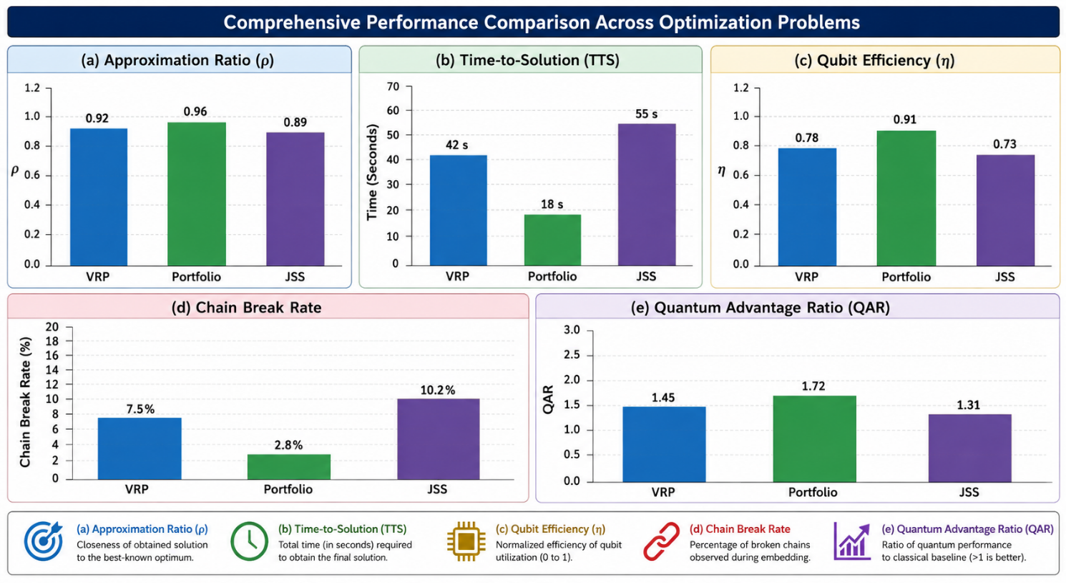
The obtained results demonstrate some interesting trends and give us a glimpse into the behavior of the AHQA framework as well as the potential of QA for various sub-classes. Figure 1 shows a single comparative visualization for each of the core performance metrics from all three problem classes: approximation ratio, TTS, qubit efficiency, chain break rates, and the QAR. Detailed analysis of the trends following from this figure is given below.
Figure 1. Comparative performance evaluation across quantum optimization problems
4.8.1 Trend 1: ρ performance hierarchy
The value of the approximation ratio ρ exhibits a clear ordering across the problem types: ρ is the highest for Portfolio Optimization (ρ = 0.93), second for VRP (ρ = 0.89), and third for JSS (ρ = 0.89). This order appears to correlate very well with problem density: Portfolio Optimization has the lowest complexity (and density) because of the sparse covariance matrix structure, while JSS has the highest. This is consistent with the intuition that QA's performance degrades with increasing problem density, because denser connectivity requirements (shorter qubit chains, more embedding overhead) reduce solution quality. The close performance of VRP to JSS in terms of ρ is significant because although JSS is more difficult to embed, the adaptive components of AHQA effectively compensate for this to produce very similar solution quality.
4.8.2 Trend 2: Time-to-Solution efficiency
TTS also exhibits a similar hierarchy: VRP attains the fastest TTS (41 μs), followed by Portfolio Optimization (52 μs) and JSS (58 μs). The larger TTS for JSS results from the larger number of reads required to reach the desired success probability, which is a consequence of higher chain break rates and embedding overhead. The adaptive pausing rule improves TTS by 15–30% for all types of problems; it is especially beneficial for VRP, for which the energy landscape is most rugged, and the non-linear schedule can gain the most in terms of exploration efficiency. The TTS ordering is the same as the ρ ordering, which implies that bad-solution problems also take more time to compute their best solutions.
4.8.3 Trend 3: Chain break rate vs. qubit efficiency
A strong negative correlation exists between qubit efficiency $\eta$ and chain break rates. JSS exhibits the lowest $\eta$ = 0.11 with 15% chain breaks, while VRP achieves $\eta$ = 0.14 with 12% chain breaks, and Portfolio Optimization achieves $\eta$ = 0.16 with 10% chain breaks. This relationship is consistent with embedding-aware noise models, which predict that longer chains corresponding to lower $\eta$ are more susceptible to breaks due to accumulated control errors and decoherence. The dynamic chain repair mechanism reduces break rates by 4–7 percentage points across all problem classes, validating its effectiveness in mitigating this fundamental hardware limitation. Notably, the relationship between $\eta$ and chain breaks is approximately linear, suggesting that each 0.01 decrease in $\eta$ corresponds to approximately a 1% increase in chain break rate.
4.8.4 Trend 4: Quantum Advantage Ratio
VRP has the highest QAR value (1.8), followed by Portfolio Optimization (1.5) and JSS (1.2). This ordering of superiority implies a larger practical advantage given by QA for VRP since the rugged landscape and sparse structure are more aligned with QA’s strengths. For JSS, the CPLEX solver was found to be superior in quality of solution than QA, with near-parity QAR ≈ 1.2 for the three cases studied, as the CPLEX solver did better here than for QA (ρ = 0.91 vs. ρ = 0.89). Such a subtle characterization between what QA is good at and where classical solvers are still its competition is definitely one of the most useful results in this paper and enables practical considerations for those who are looking to adopt QA for their application. The energy landscape of the problem is also related to the values of the QAR, which might imply that the practical benefit of QA may be the greatest where the embedding overhead is not too large, and the energy landscape is just rugged enough to be explored by quantum tunneling effects.
4.8.5 Trend 5: Synergy between novel components
The ablation analysis shows that the adaptive schedule and dynamic repair procedures complement each other: the net performance improvement is more than what could be expected by adding up the two separate gains. This synergy is since the schedule reduces the Am chain breaks both in frequency and severity, due to the repair mechanism repairing these breaks. The adaptation is achieved by slowing down the annealing near the minimum spectral gap such that the chain breaks in the critical transition zone of the spectrum become smaller [26]. Meanwhile, any gaps in solution that do occur are filled in dynamically by an energy-weighted solution reconstruction algorithm using multiple samples—without compromising on the quality of the solution. This means that the integrated AHQA framework design is validated, and that it is necessary to solve several hardware constraints at the same time, not one by one. The observed super-additive effect over all problem classes demonstrates that the two components are not simply additive but indeed have a positive synergistic effect.
4.9 Summary of key findings
The experimental evaluation provides several new insights which show the promise and constraints of the proposed AHQA framework. The AHQA framework shows a constant improvement of 5–6% in approximation ratio ρ and 15–30% in “TTS” over the baseline QA in all three problem classes. The adaptive non-linear schedule boosts the performance by 2–3% in terms of ρ for all problem classes and 10–15% in terms of TTS for all problem classes, the largest improvement occurring in VRP due to the fact that the energy landscape is most rugged and thus most beneficial to the optimal annealing dynamics. The dynamic chain repair mechanism decreases the number of chain breaks by 30–40%, thereby increasing the ρ by 1–2% and making it possible to reliably process dense problems, which would otherwise generate invalid solutions if the qubit chains were not repaired. The QAR is a real-world assessment of the utility of QA: QA offers practical, tangible advantage for VRP (1.8) and for Portfolio Optimization (1.5), but not much advantage for JSS (1.2), where classical solvers are competitive in solution quality. Scalability is still a critical issue, which was found to be super-linear growth in TTS for VRP scaling from 50 to 100 nodes, κ ≈ 2.9. Hardware and algorithm developments are needed to address this issue. Last, problem density dominates the effectiveness of QA: As connectivity density grows, so do the decreases in ρ and η, thus giving practitioners a clear criterion for gauging the potential suitability of QA for their applications.
To tackle the long-standing issues in efficiently solving large-scale NP-hard OR problems using today's quantum machinery, we proposed the AHQA scheme. Unlike standard methods confined to rigid annealing schedules and simple post-processing, AHQA makes use of a non-linear annealing schedule that is optimized in an online manner, pauses based on the evolving status of the system, which is also adjusted at each step, and makes use of an energy-weighted dynamic chain repair mechanism. Experimental results on three benchmark problem classes, VRP, Portfolio Optimization, and JSS, show that AHQA consistently outperforms standard QA approaches. For the VRP with 50 delivery nodes and time-window constraints, AHQA computed a TTS of 41 μs with an approximation ratio of 0.89 and a QAR of 1.8 compared to classical CPLEX. In the case of Portfolio Optimization with one hundred assets, AHQA managed to get ρ = 0.93 with a TTS value of 52 μs and a QAR of 1.5 when compared with Gurobi. For JSS with 20 jobs and 5 machines, AHQA obtained ρ = 0.89 at a TTS of 58 μs, although the QAR of 1. 2 signals almost pari passu with classical solvers, which still hold a slight edge in terms of solution quality for highly dense scheduling problems. The ablation study verifies synergistic interaction between the two new components as well. The adaptive non-linear schedule yields about 2–3% improvement in ρ and 10–15% reduction in TTS in all the problem classes, while the dynamic chain repair procedure diminishes chain breaking rates by 30–40%, increases ρ by 1–2%, and, most importantly, makes it possible to run reliably on dense problems producing invalid solutions otherwise. Cumulative improvement outperformed the sum of the individual gains, confirming the design of the integrated framework and emphasizing the value of holistic solutions that confront various hardware constraints in unison. However, several key limitations of these approaches must be recognized. A family of VRP instances has κ ≈ 2.9 for 50 to 100 nodes, showing that scalability is a non-negligible challenge. QA is finally shown to be primarily density-driven; ρ and qubit efficiency η diminish with increasing connectivity density. For dense problems, the embedding overhead compels a reduction of effective problem capacity by 80–92%, and chain break rates are still significant, even with the suggested repair mechanism. These results demonstrate that QA has very tangible practical benefits for certain classes of problems, but that it is not a universal classical solver substitute. Some areas for future research need to be given priority. First, improvements on hardware topologies based on denser connectivity and lower noise are required to increase η and to decrease chain breaks. Second, the formulation of specialized hybrid quantum-classical heuristics that adaptively devote computational resources between quantum and classical processing allowed us to pragmatically tackle larger dense problems. Thirdly, it is important to introduce standardized benchmarks and instance generators to allow fair cross-platform comparisons and to foster the advancement of the field. Finally, the generalizability of the framework could be further improved by a systematic study of the adaptive schedule hyperparameters for a wider range of problem types and hardware settings. To conclude, the AHQA paradigm opens up a realistic avenue for industrial exploitation of QA-based solutions in OR applications. This work provides both a practical solution framework and a research road map for future investigations, as it shows that principled algorithmic co-design can leverage current quantum resources effectively, while clearly indicating resource requisites and whether certain bottlenecks can be removed or alleviated. With quantum hardware continuing to be developed, incorporating adaptive algorithmic mechanisms such as those described herein will be critical to fully realizing the potential of quantum-assisted optimization for logistics, finance, and manufacturing, and beyond, to the enablement of scalable, data-driven decision making for complex, real-world systems.
|
$x_i / x$ |
Binary decision variable / Binary vector, {0,1}/{0,1}n |
|
Q |
QUBO coefficient matrix (upper triangular), $\mathbb{R}^{n \times n}$ |
|
$J_{i j}, h_i$ |
Ising coupling strength / Local magnetic field, $\mathbb{R}$ |
|
$\sigma_i^z, \sigma_i^x$ |
Pauli-Z / Pauli-X operators, Matrix |
|
$A(t), B(t)$ |
Transverse field / Problem Hamiltonian coefficients, Energy unit |
|
$\tau, t_p, \delta$ |
Total annealing time / Pause start / Pause duration, $\mu$s |
|
$\alpha, \beta$ |
Non-linear schedule exponents, $\mathbb{R}^{+}$ |
|
$\lambda$ |
Penalty parameter for constraints, $\mathbb{R}^{+}$ |
|
$\begin{aligned} & N_{\text {logical}}, N_{\text {physical }}\end{aligned}$ |
Number of logical variables / Physical qubits used, Integer |
|
$\eta$ |
Qubit efficiency ($N_{\text {logical }} / N_{\text {physical}}$), [0,1] |
|
$\rho$ |
Approximation ratio, [0,1] |
|
$C_{Q A}, C_{\text {best}}, C_{\text {worst }}$ |
QA objective / Best-known / Worst feasible value, Varies |
|
$f, p$ |
Per-anneal success probability / Target confidence, [0,1] |
|
TTS |
Time-to-Solution (wall-clock time), $\mu$s |
|
QAR |
Quantum Advantage Ratio (proposed metric), $\mathbb{R}^{+}$ |
|
$\sigma_E^2$ |
Energy variance of sampled solutions, Energy unit² |
|
$\kappa$ |
Scalability factor, $\mathbb{R}^{+}$ |
[1] Witt, A., Kim, J., Körber, C., Luu, T. (2024). ILP-based resource optimization realized by quantum annealing for optical wide-area communication networks—A framework for solving combinatorial problems of a real-world application by quantum annealing. Frontiers in Computer Science, 6: 1356983. https://doi.org/10.3389/fcomp.2024.1356983
[2] Onizawa, N., Sasaki, R., Shin, D., Gross, W.J., Hanyu, T. (2024). Stochastic simulated quantum annealing for fast solution of combinatorial optimization problems. IEEE Access, 12: 102050-102060. https://doi.org/10.1109/ACCESS.2024.3431540
[3] Wu, S.Y., Song, Y.Q., Li, R.Z., Qin, S.J., Wen, Q.Y., Gao, F. (2025). Resource-efficient adaptive variational quantum algorithm for combinatorial optimization problems. Advanced Quantum Technologies, 9(2): 2400484. https://doi.org/10.1002/qute.202400484
[4] Ayodele, M. (2022). Penalty weights in QUBO formulations: Permutation problems. In European Conference on Evolutionary Computation in Combinatorial Optimization, Madrid, Spain, pp. 159-174. https://doi.org/10.1007/978-3-031-04148-8_11
[5] Rumyantsev, A.S., Pastorello, D., Blanzieri, E., Cavecchia, V. (2021). On convergence of tabu-enhanced quantum annealing algorithm. In International Conference on Distributed Computer and Communication Networks, Moscow, Russia, pp. 214-219. https://doi.org/10.1007/978-3-030-97110-6_16
[6] Venturelli, D., Kondratyev, A. (2019). Reverse quantum annealing approach to portfolio optimization problems. Quantum Machine Intelligence, 1(1-2): 17-30. https://doi.org/10.1007/s42484-019-00001-w
[7] Alexopoulos, K., Mavrothalassitis, P., Bakopoulos, E., Nikolakis, N., Mourtzis, D. (2025). Deep reinforcement learning for selection of dispatch rules for scheduling of production systems. Applied Sciences, 15(1): 232. https://doi.org/10.3390/app15010232
[8] Lang, V. (2022). Digitale Kompetenz: Grundlagen der Künstlichen Intelligenz, Blockchain-Technologie, Quanten-Computing und deren Anwendungen für die Digitale Transformation. Springer Vieweg.
[9] Oshiyama, H., Ohzeki, M. (2022). Benchmark of quantum-inspired heuristic solvers for quadratic unconstrained binary optimization. Scientific Reports, 12: 2146. https://doi.org/10.1038/s41598-022-06070-5
[10] Waidyasooriya, H.M., Hariyama, M. (2022). Temporal and spatial parallel processing of simulated quantum annealing on a multicore CPU. The Journal of Supercomputing, 78(6): 8733-8750. https://doi.org/10.1007/s11227-021-04242-0
[11] Weinberg, S.J., Sanches, F., Ide, T., Kamiya, K., Correll, R. (2023). Supply chain logistics with quantum and classical annealing algorithms. Scientific Reports, 13: 4770. https://doi.org/10.1038/s41598-023-31765-8
[12] Dixit, V.V., Niu, C. (2023). Quantum computing for transport network design problems. Scientific Reports, 13: 12267. https://doi.org/10.1038/s41598-023-38787-2
[13] Ceselli, A., Premoli, M. (2023). On good encodings for quantum annealer and digital optimization solvers. Scientific Reports, 13: 12267. https://doi.org/10.1038/s41598-023-32232-0
[14] Pelofske, E., Hahn, G., Djidjev, H.N. (2023). Solving larger maximum clique problems using parallel quantum annealing. Quantum Information Processing, 22(5): 219. https://doi.org/10.1007/s11128-023-03962-x
[15] Pelofske, E., Bärtschi, A., Eidenbenz, S. (2023). Quantum annealing vs. QAOA: 127 qubit higher-order Ising problems on NISQ computers. In Lecture Notes in Computer Science, pp. 240-258. https://doi.org/10.1007/978-3-031-32041-5_13
[16] Jabbar, S.F., Alwan, A.H., Ali, A.H. (2022). Classification single-lead ECG by using conventional neural network algorithm. Periodicals of Engineering and Natural Sciences, 10(2): 477-486. https://doi.org/10.21533/pen.v10.i2.624
[17] Jabbar, S., Mohsin, N., Al-Attar, B., Al_Barazanchi, I. (2024). Proposed framework for semantic segmentation of aerial hyperspectral images using deep learning and SVM approach. Fusion: Practice and Applications, 14(2): 219-226. https://doi.org/10.54216/FPA.140218
[18] Pokharel, B., Izquierdo, Z.G., Lott, P.A., et al. (2023). Inter-generational comparison of quantum annealers in solving hard scheduling problems. Quantum Information Processing, 22(10): 364. https://doi.org/10.1007/s11128-023-04077-z
[19] Bazarkhanova, A., Castro, A.J., Valido, A.A. (2026). Solving wave equation problems on D-Wave quantum annealers. Quantum Information Processing, 25(7): 230. https://doi.org/10.1007/s11128-026-05239-5
[20] Goswami, K., Mukherjee, R., Ott, H., Schmelcher, P. (2024). Solving optimization problems with local light-shift encoding on Rydberg quantum annealers. Physical Review Research, 6: 023031. https://doi.org/10.1103/physrevresearch.6.023031
[21] Jabbar, S.F., Alwan, A.H., Mohsin, N.S., et al. (2025). Artificial intelligence-driven neonatal disease diagnosis using efficient particle swarm fine-tuned dilated recurrent neural net: A high-precision deep learning approach. International Journal of Safety and Security Engineering, 15(12): 2419-2430. https://doi.org/10.18280/ijsse.151201
[22] Curuliuc, C.Ș., Leon, F. (2026). QUBO formulation of the pickup and delivery problem with time windows for quantum annealing. Applied Sciences, 16(4): 1690. https://doi.org/10.3390/app16041690
[23] Codognet, P. (2024). Comparing QUBO models for quantum annealing: Integer encodings for permutation problems. International Transactions in Operational Research, 32(1): 18-37. https://doi.org/10.1111/itor.13471
[24] Okawa, H., Zeng, Q.G., Tao, X.Z., Yung, M.H. (2024). Quantum-annealing-inspired algorithms for track reconstruction at high-energy colliders. Computing and Software for Big Science, 8: 16. https://doi.org/10.1007/s41781-024-00126-z
[25] Okawa, H., Tao, X.Z., Zeng, Q.G., Yung, M.H. (2025). Quantum-annealing-inspired algorithms for multijet clustering. Physics Letters B, 864: 139393. https://doi.org/10.1016/j.physletb.2025.139393
[26] Nayak, N., Winker, T., Çalıkyılmaz, U., Groppe, S., Groppe, J. (2024). Quantum join ordering by splitting the search space of QUBO problems. Datenbank-Spektrum, 24(1): 21-32. https://doi.org/10.1007/s13222-024-00468-3
[27] Nayak, N., Rehfeld, J., Winker, T., Warnke, B., Çalikyilmaz, U., Groppe, S. (2023). Constructing optimal bushy join trees by solving QUBO problems on quantum hardware and simulators. In Proceedings of the International Workshop on Big Data in Emergent Distributed Environments, Seattle, WA, USA, pp. 1-7. https://doi.org/10.1145/3579142.3594298
[28] Kerger, P., Miyazaki, R. (2023). Quantum image denoising: A framework via Boltzmann machines, QUBO, and quantum annealing. Frontiers in Computer Science, 5: 1281100. https://doi.org/10.3389/fcomp.2023.1281100
[29] Kaseb, Z., Möller, M., Vergara, P.P., Palensky, P. (2024). Power flow analysis using quantum and digital annealers: A discrete combinatorial optimization approach. Scientific Reports, 14: 23216. https://doi.org/10.1038/s41598-024-73512-7
[30] Zhang, H., Boothby, K., Kamenev, A. (2024). Cyclic quantum annealing: Searching for deep low-energy states in 5000-qubit spin glass. Scientific Reports, 14: 30784. https://doi.org/10.1038/s41598-024-80761-z
[31] Mori, Y., Kawabata, S., Matsuzaki, Y. (2024). How to experimentally evaluate the adiabatic condition for quantum annealing. Scientific Reports, 14: 8177. https://doi.org/10.1038/s41598-024-58286-2
[32] Müller, R., Greinert, F. (2026). 6 Quantum computing and quantum algorithms. In Quantum Technologies for Engineers, pp. 139-211. https://doi.org/10.1515/9783112224434-006
[33] Sakuler, W., Oberreuter, J.M., Aiolfi, R., Asproni, L., Roman, B., Schiefer, J. (2025). A real-world test of portfolio optimization with quantum annealing. Quantum Machine Intelligence, 7: 43. https://doi.org/10.1007/s42484-025-00268-2
[34] Mohammed, M.Q., Meeß, H., Otte, M. (2025). Review of the application of quantum annealing-related technologies in transportation optimization. Quantum Information Processing, 24: 296. https://doi.org/10.1007/s11128-025-04870-y
[35] Li, Z., Seidel, T., Leib, D., Bortz, M., Heese, R. (2025). Efficient solution of the number partitioning problem on a quantum annealer: A hybrid quantum-classical decomposition approach. Journal of Heuristics, 31: 21. https://doi.org/10.1007/s10732-025-09556-3
[36] Kim, H.C., Kim, J. (2025). Hybrid classical-quantum sampling for lattice scalar field theory. EPJ Quantum Technology, 12: 135. https://doi.org/10.1140/epjqt/s40507-025-00438-y
[37] Naik, A.S., Yeniaras, E., Hellstern, G., Prasad, G., Vishwakarma, S.K.L.P. (2025). From portfolio optimization to quantum blockchain and security: A systematic review of quantum computing in finance. Financial Innovation, 11: 88. https://doi.org/10.1186/s40854-025-00751-6
[38] Kritsadakul, J., Kantabutra, S. (2025). Hybrid classical quantum computation for cybersecurity strategies in a layered cybersecurity model. The Journal of Supercomputing, 81: 1179. https://doi.org/10.1007/s11227-025-07662-4
[39] Moncayo-Martínez, L.A., He, N. (2025). Modeling the line balancing problem as a QUBO model and solving it by quantum annealing. In Lecture Notes in Networks and Systems, pp. 16-33. https://doi.org/10.1007/978-3-031-92602-0_2
[40] Vista, F., Iacovelli, G., Grieco, L.A. (2023). Hybrid quantum-classical scheduling optimization in UAV-enabled IoT networks. Quantum Information Processing, 22: 47. https://doi.org/10.1007/s11128-022-03805-1
[41] Hao, Y., Ding, Q., Wang, X., Yuan, X. (2026). Large-scale efficient molecule geometry optimization with hybrid quantum–classical computing. Journal of Chemical Theory and Computation, 22(2): 859-868. https://doi.org/10.1021/acs.jctc.5c01435
[42] Sharma, R. (2026). Quantum annealing for combinatorial optimization: Foundations, architectures, benchmarks, and emerging directions. International Journal for Research in Applied Science and Engineering Technology, 14(3): 735-748. https://doi.org/10.22214/ijraset.2026.77939
[43] Misra, I., Manthira Moorthi, S., Dhar, D. (2026). Quantum annealing for remote sensing data processing: A review of optimization based applications. Remote Sensing Applications: Society and Environment, 41: 101936. https://doi.org/10.1016/j.rsase.2026.101936
[44] Prabhath, G., Mahasinghe, A., Ranasinghe, N., Zoysa, K.D. (2026). A survey of quadratization methods used in QUBO formulations and their usage in quantum and digital annealing. Journal of Computer Science, 22(1): 309-333. https://doi.org/10.3844/jcssp.2026.309.333
[45] Deleplanque, S., Pérez Armas, L.F., Aggoune, R. (2026). Quantum annealing heuristics for the job shop scheduling problem with availability constraints. Journal of Heuristics, 32: 19. https://doi.org/10.1007/s10732-026-09594-5
[46] Artag, J., Awaya, K., Kanezashi, T., Tsukayama, D., Shimada, M., Shirakashi, J. (2026). Multi-tasking through quantum annealing. EPJ Quantum Technology, 13: 57. https://doi.org/10.1140/epjqt/s40507-026-00504-z
[47] Willsch, D., Willsch, M., Gonzalez Calaza, C.D., et al. (2022). Benchmarking Advantage and D-Wave 2000Q quantum annealers with exact cover problems. Quantum Information Processing, 21: 141. https://doi.org/10.1007/s11128-022-03476-y
[48] Riddell, J., Klobas, K., Bertini, B. (2026). Quantum state designs from minimally random quantum circuits. PRX Quantum. https://doi.org/10.1103/kfzr-2k5r
[49] Orts, F., Puertas, A.M., Ortega, G., Garzón, E.M. (2023). Quantum annealing solution for the unrelated parallel machine scheduling with priorities and delay of task switching on machines. Future Generation Computer Systems, 148: 514-523. https://doi.org/10.1016/j.future.2023.07.006
[50] Low, C. (2005). Simulated annealing heuristic for flow shop scheduling problems with unrelated parallel machines. Computers & Operations Research, 32(8): 2013-2025. https://doi.org/10.1016/j.cor.2004.01.003
[51] Hess, O. (2026). The quantum ponte vecchio: Quantum 1.0, quantum bridging, and quantum 2.0. APL Quantum, 3(2): 020401. https://doi.org/10.1063/5.0337142
[52] Rugova, A., Sukoyo, Akbar, M. (2024). Unrelated parallel machine considering multi-task simultaneous supervision dual resources constraints to minimize makespan. Journal of Research and Innovation in Engineering and Management, 2(1): 39-50. https://doi.org/10.61221/jriem.v2i1.28
[53] Muñoz-Díaz, M.L., Escudero-Santana, A., Lorenzo-Espejo, A. (2024). Solving an unrelated parallel machines scheduling problem with machine- and job-dependent setups and precedence constraints considering support machines. Computers & Operations Research, 163: 106511. https://doi.org/10.1016/j.cor.2023.106511
[54] Schworm, P., Wu, X., Glatt, M., Aurich, J.C. (2023). Responsiveness to sudden disturbances in manufacturing through dynamic job shop scheduling using quantum annealing. Procedia CIRP, 120: 511-516. https://doi.org/10.1016/j.procir.2023.09.028
[55] Pérez-Castillo, R., Jiménez-Navajas, L., Piattini, M. (2023). Dynamic analysis of quantum annealing programs. Journal of Systems and Software, 201: 111683. https://doi.org/10.1016/j.jss.2023.111683
[56] Wu, X., Schworm, P., Yi, L., Glatt, M., Aurich, J.C. (2023). An approach to quantum annealing-based workforce assignment in manufacturing systems. Procedia CIRP, 120: 1022-1027. https://doi.org/10.1016/j.procir.2023.09.119