Mustafa Al-Saffar* | Sura Z. Al-Rashid
© 2026 The authors. This article is published by IIETA and is licensed under the CC BY 4.0 license (http://creativecommons.org/licenses/by/4.0/).
OPEN ACCESS
Deep learning-based genomic variant calling has improved the accuracy of small-variant detection, but the computational requirements of existing callers remain a barrier for large-scale and resource-limited applications. In DeepVariant, candidate variants are represented as multi-channel pileup tensors, where partially redundant evidence channels increase input complexity and computational overhead. This study proposes an information-preserving Unified_Evidence encoding strategy that consolidates two semantically coupled channels into a single ordered representation while maintaining all distinguishable allelic states. The proposed encoding reduces the DeepVariant input tensor from 100 × 221 × 6 to 100 × 221 × 5 without modifying the core Inception-v3 architecture. The method is evaluated using Genome in a Bottle (GIAB) v4.2.1 benchmark data under whole-genome sequencing at different coverage levels, difficult genomic regions, inter-sample validation, and whole-exome sequencing scenarios. Experimental results show that the proposed representation decreases training time by 7.97% while introducing minimal F1-score changes for single-nucleotide polymorphism (SNP) and insertion-deletion (INDEL) detection (0.0005 and 0.0020, respectively). Moreover, under extremely low coverage conditions (5×), the proposed encoding improves average SNP and INDEL F1-scores by 0.014 and 0.020, respectively, compared with the original representation. These findings demonstrate that input-level tensor optimization provides an effective complementary direction to model compression techniques and offers a practical approach for improving the efficiency of DeepVariant-based genomic variant calling.
genomic variant calling, DeepVariant-based analysis, input tensor optimization, channel encoding, deep learning, computational efficiency, bioinformatics
Precision medicine depends on accurate computational analysis of genomic data. As high-throughput sequencing has scaled, reconciling raw reads with trustworthy genetic inferences has become an increasingly demanding task. Variant calling, the detection of deviations from a reference sequence, is now dominated by deep-learning frameworks [1]. DeepVariant [2] reframes the problem as supervised image classification over multi-channel pileup images and uses an Inception-v3 Convolutional Neural Network (CNN) [3] to learn error profiles directly from aligned-read data. This learning-based approach has substantially outperformed traditional statistical callers, particularly under the structural complexity and noise characteristic of next-generation sequencing data.
Although deep-learning models offer excellent discriminative accuracy, their adoption in resource-constrained environments is limited by high computational cost [4]. DeepVariant represents the genomic evidence at a putative variant locus as a six-channel high-dimensional tensor encoding base identity, base quality, mapping quality, strand, read_supports_variant, and base_differs_from_ref on separate planes. The last two planes are semantically coupled: both are derived from the same (observed base, reference base, alternate allele) triple, and their activations are strongly correlated on a per-pixel basis. Because the first convolutional layers operate over the full tensor depth, this redundancy translates directly into inflated Floating-Point Operation (FLOP) counts, higher Graphics Processing Unit (GPU)-memory bandwidth, and longer training cycles [5].
Despite these costs, the input-layer representation has received comparatively little attention in the optimization literature. Prior efficiency work on deep variant callers has instead targeted the classifier itself: weight quantization [6], pruning [7], lightweight backbones [8], and variant-triage schemes such as Clair3 [9]. These approaches are subtractive and operate downstream of the input encoding, which is left unchanged. We address this gap by proposing an optimized DeepVariant framework centered on the Unified_Evidence channel, a deterministic input re-encoding. This encoding fuses the two semantically coupled planes into a single dense state-indexed grayscale channel and reduces the input depth from six to five without discarding any distinguishable allelic state. Because the modification is confined to the input stem, the Inception-v3 backbone is kept intact apart from the stem depth, so any observed efficiency or accuracy effect is attributable to the representation rather than to architectural redesign. The framework is therefore positioned as a tensor-engineering complement to model-centric methods rather than a competitor. We hypothesize that, for Genome in a Bottle (GIAB) v4.2.1 [10] Whole-Genome Sequencing (WGS) data on GRCh38 [11], the proposed encoding will reduce training wall-time by at least 5%, preserve held-out F1 within |ΔF1| ≤ 0.005 at standard coverage (≥20×), and yield a non-negative F1 difference at low coverage (≤5×). Each clause is tested in Section 4.
This work makes three main contributions. First, it introduces a deterministic channel-fusion encoding (Unified_Evidence), formalized as a state-indexed mapping (Section 3.3) and implemented through a parallelizable construction algorithm. Second, it provides a controlled empirical characterization of the resulting efficiency–accuracy trade-off on the DeepVariant v1.9.0 backbone, showing a 7.97% training-time reduction at a mean F1 cost of 0.0005 (single nucleotide polymorphism (SNP)) and 0.0020 (insertion-deletion (INDEL)) over 21 paired observations. Third, it reports a controlled benchmark against DeepVariant v1.9.0, Clair3, Genome Analysis Toolkit (GATK), Octopus, Strelka2, and FreeBayes across WGS chromosome holdout, inter-sample generalization, GIAB difficult regions, a 30×/20×/5× coverage stress test, and cross-domain Whole-Exome Sequencing (WES).
The novelty of this work lies in where the optimization is applied, not in how aggressively the model is compressed. Conventional efficiency techniques for deep variant callers are subtractive and model-centric: quantization lowers numerical precision, pruning removes weights, and lightweight-backbone substitution replaces the classifier. Each of these techniques trades representational capacity for speed while operating downstream of an input tensor that is left unchanged. The Unified_Evidence encoding instead acts at the input layer and is information-preserving: the state-indexed mapping M is injective over the five distinguishable allelic states (Section 3.3), so no distinguishable evidence is discarded, and the Inception-v3 backbone is kept almost in full. The proposed encoding is therefore not an alternative to compression but a complement to it, and it can be combined with quantization, pruning, or a lighter backbone. It thus isolates the input representation as an independent and previously under-explored axis for reducing the cost of DeepVariant-class callers.
The remainder of this paper is organized as follows. Section 2 reviews variant-calling paradigms and DeepVariant-class optimization. Section 3 formalizes the Unified_Evidence representation. Section 4 reports the experimental protocol and results. Section 5 concludes.
2.1 Deep learning-based variant calling paradigms
Early variant-calling workflows were dominated by probabilistic and statistical models. GATK HaplotypeCaller [12], FreeBayes [13], and SAMtools/BCFtools [14] combine hidden Markov models with Bayesian inference [15] to estimate genotype likelihoods from aligned reads. These methods perform reliably on routine germline calling but rely on hand-crafted filters and degrade on noisy or structurally complex regions where their underlying assumptions do not hold.
Deep learning reframed variant calling as a supervised image-classification problem. Poplin et al. [2] serialized pileups of aligned reads at each candidate locus into multi-channel tensors. These tensors are analogous to RGB images but are extended to encode bases, quality indicators, and strand information. An Inception-v3 CNN trained over them achieved markedly higher accuracy than heuristic callers without manual feature design. Recent surveys of AI-based variant callers document this shift across a range of tools and sequencing technologies [16]. Subsequent work has extended this paradigm: DeNovoCNN [17] adapts the architecture to de novo calling in trio data; Clair3 [9] introduces a hybrid pileup + full-alignment triage; and contemporary DeepVariant evaluations continue to be benchmarked against expanded truth sets [18]. The present study is deliberately narrower: we examine whether an input-tensor modification can improve DeepVariant-class efficiency without altering the classifier. Table 1 summarizes the callers benchmarked here, organized by paradigm, input representation, and position relative to the input-redundancy gap addressed in this work.
Table 1. Comparative inventory of variant callers benchmarked in this study
|
Caller |
Paradigm |
Input Representation |
Position Relative to the Input-Redundancy Gap |
|
DeepVariant [2] |
CNN over pileup (Inception-v3) |
100 × 221 × 6 tensor |
Inherits redundant encoding |
|
Clair3 [9] |
Hybrid pileup + full-alignment |
Pileup + alignment |
Optimizes classifier; encoding unchanged |
|
GATK [12], FreeBayes [13], SAMtools [14] |
Probabilistic |
Aligned reads |
Orthogonal to the gap |
|
DeNovoCNN [17] |
CNN |
DV-style multi-channel |
Inherits redundant encoding |
|
Octopus [19] |
Haplotype-aware probabilistic |
Aligned reads |
Orthogonal to the gap |
|
Strelka2 [20] |
Pileup-based statistical |
Aligned reads |
Orthogonal to the gap |
|
Proposed |
CNN over re-encoded pileup |
100 × 221 × 5 tensor |
Targets encoding directly |
Note: CNN = Convolutional Neural Network, GATK = Genome Analysis Toolkit.
2.2 Computational optimization of deep variant callers
Existing efficiency work on DeepVariant-class callers can be organized into three families that all operate downstream of the input encoding. The first is parameter-level compression: quantization from FP32 to lower-precision formats [6], and structured or unstructured pruning [7]. The second is backbone substitution, in which the heavy Inception-v3 classifier [3] is replaced by mobile-class architectures via neural architecture search or manual redesign [8]; a recent example replaces the Inception-v3 backbone with a mid-sized EfficientNet and reports faster convergence and roughly half the parameters at comparable accuracy [21]. The third is computation triage, exemplified by Clair3 [9], which routes easy candidates to a lightweight network and reserves a heavier full-alignment network for ambiguous loci. These model-centric efforts, including concurrent backbone modernization [21], are orthogonal to the input-level re-encoding proposed here and could be combined with it rather than replaced by it. All three families are subtractive and tend to reduce sensitivity for under-represented variant classes, particularly INDELs and low-coverage calls [22]. They also leave the input pileup tensor unchanged, so its structural redundancy is inherited rather than removed. To our knowledge, no prior work on DeepVariant-class callers has explicitly treated the input tensor itself as an optimization target. The present study fills that gap and is designed to be composable with model-centric methods rather than to replace them.
3.1 Overview of the multi-phase strategy
The framework is built around a single design principle: before any learned transformation is applied, the pileup tensor is re-encoded so that semantically coupled evidence channels are consolidated into one information-preserving plane. The re-encoding is deterministic, non-subtractive, and architecturally minimal. Every pileup is mapped to the same output tensor regardless of training or batching. Every allelic state distinguishable in the original six-channel tensor remains distinguishable in the fused channel. Finally, the modification is confined to the input stem of the Inception-v3 backbone [3], leaving the trainable-parameter count nearly unchanged. The framework is organized into four phases: diagnostic analysis, mapping logic, tensor construction, and architectural integration. Figure 1 illustrates the complete pipeline. The baseline DeepVariant pipeline [2] is recovered exactly by replacing Stage 2 with the standard six-channel encoding, providing a one-factor comparison.

Figure 1. Logic-driven Unified_Evidence DeepVariant pipeline
3.2 Phase 1: Diagnostic analysis
The workflow ingests a reference genome (FASTA) and aligned reads (BAM, accessed via SAMtools/BCFtools [14]). Candidate sites are identified where the aligned data reveal a mismatch or insertion/deletion relative to the reference. For each candidate site i, a local genomic window of overlapping reads is assembled into a feature matrix.
Let $W_{\mathrm{i}}$ denote the read-window matrix at candidate site i. Then
$W_i=\left[r_{i, 1}, r_{i, 2}, \ldots, r_{i, N}\right]$ (1)
where, $r_{i, j}$ represents the $j$-th aligned read spanning the site, and $N$ denotes the read depth. In the baseline DeepVariant encoding [2], these windows are serialized into a six-channel tensor of shape 100 × 221 × 6.
To justify consolidation, we performed a pixel-level correlation analysis across 50,000 pileup images from the HG001 training set. This analysis computed the Pearson correlation coefficient  and mutual information (MI) between the flattened activations of read_supports_variant and base_differs_from_ref. The analysis revealed near-perfect linear correlation (r > 0.98) and high MI, confirming that the two channels carry semantically duplicated signal and that the early convolutional layers spend FLOPs on redundant feature extraction (Figure 2).

Figure 2. Quantitative redundancy analysis of the DeepVariant input channels
3.3 Phase 2: Unified_Evidence mapping
The correlation analysis in Section 3.2 establishes that the two planes are redundant; the mapping defined next converts that redundancy into a single ordered channel without discarding any distinguishable state.
At every position $(i, j)$ the joint biological evidence is described by three observables: the observed base $b^{\text {obs}}$, the reference base $b^{\text {ref}}$, and the alternate-allele set $V^{\text {alt}}=\left\{v_1, v_2\right\}$. Because the two redundant channels are functions of this single triple, their joint information can be equivalently represented by a categorical variable over a five-state set: no coverage, contradictory/ambiguous evidence, reference match, primary alternate allele, and secondary alternate allele (Table 2).
Let $S$ denote the five-state allelic space and let $I \subset$ $\{0,1, \ldots, 255\}$ denote an ordered set of discrete pixel intensities. The Unified_Evidence channel $C^{\text {unified}}$ is the image obtained by applying a deterministic mapping $M: S \rightarrow$ I defined as:
$\begin{aligned} P_{(x, y)}^{\text {unified}}= & M\left(b_{o b s}, b_{r e f}, V_{a l t}\right) = & \left\{\begin{array}{cc}0 & \text { if } S=\text { No Coverage } \\ 64 & \text { if } S=\text { Contradictory/Ambiguous } \\ 128 & \text { if } b_{o b s} \equiv b_{r e f} \text { (Ref Match) } \\ 192 & \text { if } b_{o b s} \in V_{a l t_1} \text { (Alt Allele 1) } \\ 255 & \text { if } b_{o b s} \in V_{a l t_2} \text { (Alt Allele 2) }\end{array}\right.\end{aligned}$ (2)
The mapping has three properties. The first is injectivity: distinct states map to distinct intensities, so no information is discarded. The second is monotonic ordering: intensities increase with allelic-support strength, following no coverage < ambiguous < reference < primary alt < secondary alt. The third is uniform 64-level quantization, in which the constant spacing prevents any single state from dominating gradient magnitudes after normalization. Figure 3 illustrates these properties.

Figure 3. Semantic state re-encoding diagram of the Unified_Evidence channel
Algorithm 1 implements $M$ deterministically over a candidate window. The procedure is local: $P_{\mathrm{ij}}{ }^{\text {unified}}$ depends only on the i-th read and the j-th reference column, so construction is trivially parallelizable. The mapping itself is a lookup and adds negligible pre-processing overhead; the computational savings reported in Section 4 arise downstream, at the input stem of the CNN.
Let $C h^{\text {base}}, C h^{\varphi \text {ual}}, C h^{\text {map}}, C h^{\text {strand}}$ denote the four preserved evidence planes from the baseline DeepVariant encoding [2], and let $C h^{\text {unified}}$ denote the Unified_Evidence plane defined by $M$. The final five-channel input to the classifier is the concatenation:
$Input_v=\left[C h_{\text {base}}, C h_{\text {qual}}, C h_{\text {map}}, C h_{\text {strand}}, C h_{\text {unified}}\right]$ (3)
The effective feature volume per candidate site is reduced from 132,600 to 110,500 values, a 16.7% reduction at the input layer. Because the Inception-v3 stem [3] operates over the full tensor depth, this translates proportionally into fewer FLOPs at the stem.
Table 2. Mapping of allele states to grayscale pixel intensities in the Unified_Evidence channel
|
Allele State |
Pixel Intensity |
Description |
|
0 |
0 |
No coverage |
|
1 |
64 |
Contradictory evidence |
|
2 |
128 |
Reference support |
|
3 |
192 |
First alternate allele |
|
4 |
255 |
Second alternate allele |
|
Algorithm 1. Unified_Evidence Tensor Construction |
|
Input: Aligned Reads (R), Reference Genome (G), Candidate Window (W) Output: Unified_Evidence Matrix (U) of size H × W Procedure: 1: Initialize Matrix U with zeros (H, W) 2: For each column j in Window W do: 3: RefBase ← G[j] 4: For each read i spanning position j do: 5: ReadBase ← R[i, j] 6: IsAlt ← CheckVariantSupport(R[i], j) 7: 8: IF ReadBase is Missing THEN 9: U[i, j] ← 0 // No Coverage 10: ELSE IF IsAlt is Ambiguous THEN 11: U[i, j] ← 64 // Contradictory 12: ELSE IF ReadBase == RefBase THEN 13: U[i, j] ← 128 // Reference Match 14: ELSE IF ReadBase == AltAllele1 THEN 15: U[i, j] ← 192 // Alt Support 1 16: ELSE IF ReadBase == AltAllele2 THEN 17: U[i, j] ← 255 // Alt Support 2 18: END IF 19: End For 20: End For 21: Return Normalize(U) |
3.4 Phase 3-4: Architectural integration and training
Two minimal changes are made to the Inception-v3 backbone [3]. First, the input stem is re-initialized to accept 100 × 221 × 5 rather than 100 × 221 × 6, with kernel size, stride, and padding unchanged; the Inception blocks, auxiliary classifier, and head are unaltered. Second, the network emits a logit vector $z \in R^3$ over the three zygosity classes {Hom-ref, Het, Hom-alt}, with the standard Softmax posterior.
$P\left(G_{\mathrm{k}} \mid T\right)=\exp \left(\mathrm{z}_{\mathrm{k}}\right) / \sum_{\mathrm{i}=0}^2 \exp \left(\mathrm{z}_{\mathrm{i}}\right)$ (4)
The discrete intensities $\{0,64,128,192,255\}$ produced by $M$ are rescaled to the unit interval by linear normalization $T_{\text {norm}}=T_{\mathrm{ra}} w / 255$, mapping the five states onto $\{0,64 / 255$, $128 / 255,192 / 255,1\}$ with constant spacing $64 / 255 \approx 0.251$. The uniform spacing follows directly from the quantization property of M and keeps initial activations comparable in scale to the other four normalized channels, preventing the fused channel from dominating the gradients of the first convolutional filters at initialization. The model is implemented in TensorFlow [23]. Trainable parameters differ from the baseline only through the reduced filter depth at the stem; any empirical difference in accuracy, training time, or inference latency is therefore attributable to the input representation rather than to classifier-side changes.
Having defined the Unified_Evidence encoding and its integration into the Inception-v3 stem in Section 3, this section tests whether that deterministic, information-preserving re-encoding delivers the intended efficiency gains without sacrificing accuracy. Every experiment follows a strict one-factor protocol in which the proposed and baseline models differ only in the input representation, so any measured difference can be attributed to the encoding alone. The evaluation proceeds from computational efficiency (Section 4.2), through single-chromosome and multi-axis accuracy (Sections 4.3–4.4), to two deliberately adversarial settings: reduced sequencing depth (Section 4.5) and cross-domain whole-exome data (Section 4.6), before the statistical analysis in Section 4.7.
4.1 Experimental configuration
All experiments were run on a fixed workstation under a single software stack, following one-factor protocols in which the proposed model and the baseline differed only in the input representation. The complete configuration is summarized in Table 3.
To support reproducibility, the hyperparameter settings and training configuration used for both the baseline and the proposed Unified_Evidence model are summarized in Table 4.
Comparators were selected for public, actively maintained implementations with pinned releases and native GRCh38 / GIAB v4.2.1 support. Together they cover three caller families relevant to the input-representation question: DeepVariant-class deep-learning callers (DeepVariant v1.9.0 as the direct paired baseline; Clair3 as a contemporary deep-learning reference point), haplotype-aware probabilistic callers (GATK, Octopus), and pileup-based statistical callers (Strelka2, FreeBayes). Held-out chromosomes were chosen to span variation in length, GC content, MHC-region polymorphism (chr9), segmental-duplication density (chr15), and gene density (chr19); chr21 was retained for direct comparability with the GIAB benchmarking literature. The seven GIAB samples and three-chromosome stratification together yield n = 21 paired observations for the statistical analysis in Section 4.7.
The GIAB v4.2.1 resource was selected as the sole benchmark because it provides community-standard truth sets together with matched high-confidence region masks. These resources are curated by the GIAB Consortium and are the reference standard for germline small-variant benchmarking [10, 24]. Using them keeps the reported accuracies directly comparable with the wider variant-calling literature and removes truth-set choice as a confounder. The samples were chosen to exercise three distinct sources of variability. HG001 (the widely used NA12878 pilot genome) supplies the training and primary held-out data. The Ashkenazi Jewish trio (HG002, HG003, HG004) and the Han Chinese trio (HG005, HG006, HG007) extend the evaluation across different individuals, ancestries, and family structures, which is precisely what the inter-sample and difficult-region analyses in Section 4.4 require to separate a genuine representation effect from sample-specific variability. The three sequencing depths 30× (standard), 20× (moderate), and 5× (extreme sparsity) were included to support the coverage-robustness analysis in Section 4.5. The redundancy that the Unified_Evidence channel consolidates is itself coverage-dependent, so evaluating across a six-fold range of depths is essential for characterizing when the fused encoding helps and when it costs. Finally, the GIAB difficult-regions mask and the cross-domain Integrated DNA Technologies (IDT) whole-exome data probe the encoding under repeat-rich contexts and under a training–test domain shift, respectively.
Table 3. Experimental configuration
|
Category |
Specification |
|
CPU / RAM / GPU |
Intel Core i9-12900F · 16 GB DDR5 · NVIDIA RTX 3070 Ti (8 GB) |
|
OS/runtime |
Ubuntu 20.04 · Python 3.10 · CUDA 11.8 · TensorFlow 2.13.1 (FP32) [23] |
|
Reference/truth |
GRCh38 [11]; GIAB v4.2.1 [10] |
|
Training/split |
HG001, HG003, HG005 · chr1, chr10 train · chr20 validate · chr21 test |
|
Held-out chromosomes |
chr5, chr9, chr15, chr19 |
|
Inter-sample evaluation |
HG002, HG004, HG006 across chr5/19/21 |
|
Coverage stress |
HG007 across chr5/19/21 at 30×, 20×, 5× |
|
Difficult regions |
HG004, GIAB "all-difficult" mask |
|
WES evaluation |
HG002–HG004; IDT 100× deduplicated |
|
Hyperparameters |
RMSProp, batch 64, 30 epochs, lr 1 × 10⁻⁴, weight decay 4 × 10⁻⁵, dropout 0.2 |
|
Baseline callers |
DeepVariant v1.9.0 [2], Clair3 [9], GATK v4.6.2 [12], Octopus v0.7.4 [19], Strelka2 v2.9.10 [20], FreeBayes [13] |
|
Accuracy harness |
hap.py v0.3.15 [24] vs. GIAB v4.2.1 high-confidence BED, "PASS" filter |
Note: CPU = Central Processing Unit, RAM = Random Access Memory, GPU = Graphics Processing Unit, GIAB = Genome in a Bottle, GATK = Genome Analysis Toolkit, WES = Whole-Exome Sequencing, IDT = Integrated DNA Technologies, BED = Browser Extensible Data.
Table 4. Training configuration and hyperparameters (identical for baseline and proposed; the two models differ only in input-tensor depth)
|
Setting |
Value |
|
Deep-learning framework |
TensorFlow 2.13.1 (FP32) [23] |
|
Backbone |
Inception-v3 [3] (input-stem depth 6 → 5; Inception blocks, auxiliary classifier and head unchanged) |
|
Input tensor shape |
100 × 221 × 6 (baseline) / 100 × 221 × 5 (proposed) |
|
Output layer |
3-class Softmax over {Hom-ref, Het, Hom-alt} |
|
Optimizer |
RMSProp |
|
Learning rate |
1 × 10⁻⁴ |
|
Weight decay |
4 × 10⁻⁵ |
|
Dropout |
0.2 |
|
Batch size |
64 |
|
Training epochs |
30 |
|
Loss function |
Categorical cross-entropy |
|
Input normalization |
Linear, Tnorm = Traw / 255 |
|
Trainable parameters |
≈21.77 M (both models) |
All accuracy metrics are produced by hap.py [24] against the GIAB v4.2.1 high-confidence Browser Extensible Data (BED) with PASS-filter retention; all runtimes are end-to-end wall-clock measurements. Timings are single-run point values; replicated runs with variance estimation are identified as future work. Per-sample and per-chromosome breakdowns of every result reported in Sections 4.2–4.7 (training-log summary, chromosome holdout, coverage stress test, inter-sample holdout, GIAB difficult-region stratification, per-sample WES benchmark, and the paired statistical test) are provided as Tables A1–A7 in the Appendix.
Evaluation uses precision, recall, and their harmonic mean, the F1-score, computed separately for SNPs and INDELs. These metrics are reported because variant calling is a strongly class-imbalanced detection task: true variants are rare relative to the number of reference and candidate positions examined, so plain accuracy is dominated by true negatives and can stay high even when many real variants are missed. Precision measures the fraction of reported calls that are genuine and therefore reflects the false-positive burden, which is critical in a clinical setting where spurious calls can trigger unnecessary follow-up. Recall (sensitivity) measures the fraction of true variants that are recovered and therefore reflects the false-negative burden, which is critical when a missed variant may be clinically actionable. Because precision and recall trade off against one another, the F1-score summarizes both in a single value and allows a fair one-number comparison between callers. Precision, recall, and F1-score as computed by hap.py against the GIAB high-confidence regions are also the metrics adopted in the established germline-benchmarking guidance [24], so their use keeps the present results directly comparable with prior work.
4.2 Computational efficiency
The Unified_Evidence representation reduces training wall-time by 7.97% (19 h 05 m → 17 h 34 m) and lowers input-layer feature volume by 16.7%, at a paired F1 cost of 0.0005 (SNP) and 0.0020 (INDEL) across 21 paired observations, with all six paired t-tests significant at p < 0.001.
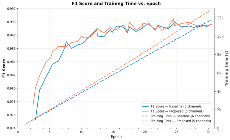
Under the protocol of Table 3, the proposed five-channel architecture reduces total training wall-time by 7.97% relative to the six-channel baseline (Table 5). Example generation (make_examples) and example shuffling are essentially unchanged, so the reduction is concentrated in the training loop, consistent with the stem-only FLOP reduction. Input-stem FLOPs per sample decrease from 2.011 × 10⁹ to 2.008 × 10⁹, and the trainable-parameter count is nearly unchanged (~21.77 M in both models). At the training-log level, all accuracy changes are small and uniformly negative (categorical accuracy −0.00068, weighted F1 −0.00068, per-class F1 ≤ 0.00076), corresponding to 227 additional false negatives and 217 additional false positives over a validation pool of 981,594 examples. Convergence is stable throughout the 30-epoch horizon (Figure 4).
To explain why the re-encoding lowers training time, it is useful to separate the pipeline into data preparation and model training. Example generation (make_examples) and example shuffling operate on the read-level data before the tensor is consumed by the network and are therefore essentially unchanged between the two configurations (a +48 s difference in make_examples and a −5 m 52 s difference in shuffling, both within normal run-to-run variation). The saving is concentrated in the training loop, which is where the input representation actually matters. Consolidating two coupled planes into one reduces the input tensor from 100 × 221 × 6 to 100 × 221 × 5, a 16.7% reduction in the number of values that enter the network at every step. This smaller tensor lowers both the computation and, more importantly, the memory traffic at the input stem for each of the roughly one million training examples processed in each of the thirty epochs; although the per-step reduction is small, it accumulates over the full training horizon into the observed wall-time reduction. Because the Inception blocks, the auxiliary classifier, and the trainable-parameter count (≈ 21.77 M) are all left unchanged, this saving is attributable to the lighter input representation rather than to any reduction in model capacity.
Having established that the encoding reduces training cost, the next question is whether this saving is paid for in accuracy; the following sections quantify the accuracy side of the trade-off, beginning with the held-out chromosome.
Table 5. Training-log summary; baseline vs. proposed under identical hyperparameters
|
Metric |
Baseline |
Proposed |
Δ |
|
Make_example time |
01:11:23 |
01:12:11 |
+0:48 |
|
Shuffle time |
01:24:16 |
01:18:24 |
−5:52 |
|
Training time |
19:05:26 |
17:34:08 |
−7.97% |
|
F1 (weighted) |
0.9957 |
0.9951 |
−0.00068 |
Figure 4. Training dynamics over 30 epochs: validation F1 (left axis) and cumulative wall time (right axis) for baseline and proposed models
4.3 Whole-Genome Sequencing benchmark on the held-out chromosome
Inference is evaluated on the held-out chr21 of HG001 at 30× WGS coverage. Table 6 compares the proposed framework with six baseline callers under identical conditions. The proposed framework achieves the lowest inference time among the seven callers (2 m 47 s), marginally faster than the baseline (2 m 49 s). It is approximately 4.2× faster than Clair3, 3.7× faster than Octopus, and 7.5× faster than Strelka2. Accuracy is essentially preserved: SNP F1 = 0.9952 (baseline 0.9957, Δ = −0.0005) and INDEL F1 = 0.9876 (baseline 0.9893, Δ = −0.0017). Clair3 retains a narrow accuracy lead at approximately 4× the runtime.
Table 6. Accuracy and runtime on HG001 chr21, 30× WGS, GRCh38
|
Caller |
Runtime |
SNP F1 |
INDEL F1 |
|
Proposed Framework |
02:47 |
0.9952 |
0.9876 |
|
Baseline DeepVariant |
02:49 |
0.9957 |
0.9893 |
|
Clair3 |
11:33 |
0.9959 |
0.9928 |
|
GATK |
14:09 |
0.9917 |
0.9922 |
|
Octopus |
10:19 |
0.9919 |
0.9897 |
|
FreeBayes |
03:46 |
0.9813 |
0.9749 |
|
Strelka2 |
21:00 |
0.9941 |
0.9911 |
Note: GATK = Genome Analysis Toolkit, WGS = Whole-Genome Sequencing, SNP = single nucleotide polymorphism, INDEL = insertion-deletion.
4.4 Generalization across chromosomes, samples, and difficult regions
A single held-out chromosome cannot by itself show whether the encoding is stable across the genome and across individuals, so the three generalization axes below address this directly.
The framework was therefore evaluated along three orthogonal generalization axes (Table 7).
Table 7. Generalization across cross-chromosome, inter-sample, and difficult-region axes (all at 30× WGS, GRCh38)
|
Panel |
Stratum |
Caller |
SNP F1 |
INDEL F1 |
|
A. Cross-chromosome (HG001, mean over chr5/9/15/19/21) |
mean [min, max] |
Baseline |
0.9945 [0.9924, 0.9957] |
0.9874 [0.9858, 0.9893] |
|
|
Proposed |
0.9942 [0.9923, 0.9954] |
0.9857 [0.9837, 0.9876] |
|
|
|
Clair3 |
0.9946 [0.9924, 0.9959] |
0.9930 [0.9921, 0.9944] |
|
|
B. Inter-sample (mean over chr5/19/21) |
HG002 |
Baseline |
0.9943 |
0.9868 |
|
Proposed |
0.9936 |
0.9842 |
||
|
Clair3 |
0.9953 |
0.9934 |
||
|
HG004 |
Baseline |
0.9948 |
0.9873 |
|
|
Proposed |
0.9941 |
0.9856 |
||
|
Clair3 |
0.9957 |
0.9946 |
||
|
HG006 |
Baseline |
0.9872 |
0.9720 |
|
|
Proposed |
0.9869 |
0.9691 |
||
|
Clair3 |
0.9836 |
0.983 |
||
|
C. Difficult regions (HG004, GIAB all-difficult, mean over chr5/19/21) |
|
Baseline |
0.9767 |
0.9825 |
|
|
Proposed |
0.9751 |
0.9807 |
|
|
|
Clair3 |
0.9803 |
0.9928 |
Note: WGS = Whole-Genome Sequencing, SNP = single nucleotide polymorphism, INDEL = insertion-deletion, GIAB = Genome in a Bottle.
Cross-chromosome generalization on five held-out chromosomes of HG001 yields proposed SNP F1 $\in$ [0.9923, 0.9954] and INDEL F1 $\in$ [0.9837, 0.9876], confirming that the chr21 result is representative. Inter-sample generalization on three additional GIAB samples yields a consistent representation gap of |ΔF1| ≤ 0.0007 (SNP) and |ΔF1| ≤ 0.003 (INDEL); the larger absolute drop on HG006 affects both DeepVariant-class models and reflects sample-level variability rather than a representation effect. Under the GIAB "all-difficult" mask, the representation gap remains ≤ 0.0018, indicating that the fused channel does not disproportionately degrade in repeat-rich, segmental-duplication, or GC-skewed contexts. Across all three axes, |ΔF1| ≤ 0.003 on both variant classes, with no axis revealing a regime in which the fused channel collapses.
4.5 Robustness under reduced sequencing depth
The analyses so far hold coverage fixed at 30×. Because the redundancy that the encoding removes is coverage-dependent, the behavior of the fused channel under reduced depth is examined next.
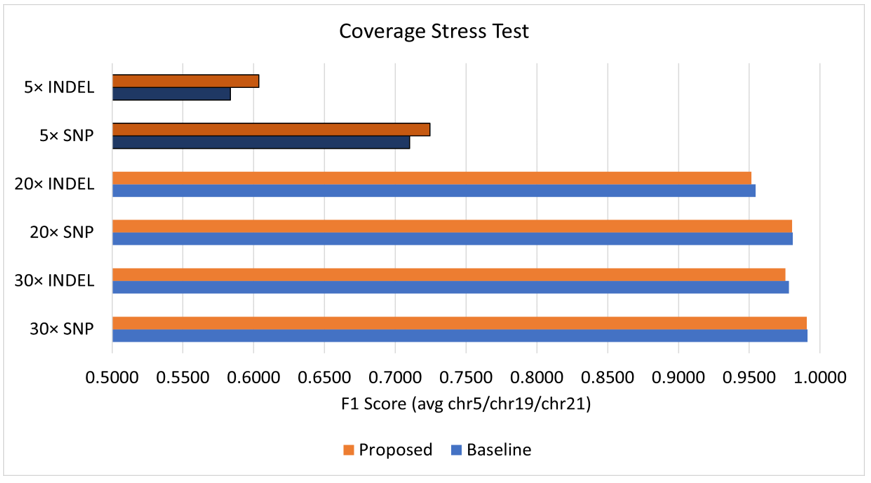
Coverage robustness was characterized on HG007 across chr5/19/21 at 30× (standard), 20× (moderate), and 5× (extreme sparsity). Three patterns emerged (Table 8, Figure 5). At 30×, the two models tracked each other within 0.002 SNP F1 and 0.004 INDEL F1. At 20×, the gap remained small. At 5×, the direction reversed: the proposed framework outperformed the baseline on every chromosome for both variant classes, with mean gains of +0.014 SNP F1 and +0.020 INDEL F1.
The reason the fused encoding changes sign at 5× can be traced to how the two source planes behave as coverage falls. At 30× and 20×, the read_supports_variant and base_differs_from_ref planes are near-duplicates (pixel-level correlation r > 0.98, Section 3.2), so fusing them is almost lossless and the proposed model tracks the baseline to within 0.0004 SNP F1 and about 0.003 INDEL F1. The small negative differences at these depths reflect rare boundary cases rather than a systematic weakness. At 5×, sparse and uneven read support breaks this correlation: pixels for which one plane fires while the other does not become common and correspond to genuinely ambiguous evidence (for example, CIGAR or soft-clip artifacts, allele-set mis-registration, or base-quality discordance). In the six-channel baseline, these pixels appear as two mutually inconsistent binary signals on separate planes, which the classifier must reconcile and often resolves inconsistently. In the fused channel, the same pixels collapse onto a single explicit ambiguous state at intensity 64, ordered distinctly from the reference (128) and alt-supporting (192, 255) states. This gives the network a single explicit, learnable state for low-confidence evidence that both the SNP and INDEL decision boundaries can down-weight, producing the observed mean gains of +0.014 SNP F1 and +0.020 INDEL F1. The advantage should be read in context: absolute F1 at 5× remains below 0.77 for both deep-learning models, so the fused encoding delivers a consistent relative improvement inside an intrinsically high-error regime, not a recovery of standard-depth accuracy.
Table 8. HG007 coverage stress test, chromosome-averaged F1 (chr5/19/21)
|
Coverage |
Baseline SNP / INDEL |
Proposed SNP / INDEL |
Δ SNP / INDEL |
|
30× |
0.9910 / 0.9780 |
0.9907 / 0.9755 |
−0.0003 / −0.0025 |
|
20× |
0.9807 / 0.9546 |
0.9803 / 0.9515 |
−0.0004 / −0.0031 |
|
5× |
0.7101 / 0.5835 |
0.7245 / 0.6037 |
+0.0144 / +0.0202 |
Note: SNP = single nucleotide polymorphism, INDEL = insertion-deletion.
Figure 5. Chromosome-averaged F1 on HG007 at 30×, 20×, and 5×
4.6 Whole-exome sequencing
Reduced depth stresses the encoding within the whole-genome domain; the whole-exome evaluation now stresses it across domains, since both deep-learning models are trained on whole-genome data.
The WES evaluation uses the IDT 100× deduplicated dataset for HG002, HG003, and HG004. Both DeepVariant-class models are trained on WGS and therefore tested in a cross-domain configuration; Clair3 [9] is included as a contemporary deep-learning reference (Table 9). Two observations follow. First, both WGS-trained DeepVariant-class models lose substantial sensitivity on cross-domain WES relative to the in-domain WGS holdout, as expected for a training–test domain mismatch [25]. Second, the Unified_Evidence representation shifts the WES operating point toward higher precision at the cost of recall: averaged across HG002–HG004, INDEL precision rises from 0.904 to 0.921 while INDEL recall falls from 0.522 to 0.421. SNP precision is essentially unchanged (0.9924 → 0.9928). Fusing two semantically coupled channels into a single ordered state yields a denser, slightly more conservative input signal in exon-dense regions and pushes the classifier toward higher-specificity decisions. Clair3 substantially outperforms both WGS-trained pipelines on WES (SNP F1 = 0.977, INDEL F1 = 0.894), confirming that the dominant factor on this dataset is training-domain match rather than input-representation depth. Figure 6 shows the corresponding precision–recall trade-off for both variant classes.
Table 9. WES benchmarking on the Ashkenazim Trio (IDT 100×), sample-averaged
|
Caller |
Type |
Average Runtime |
Average F1 |
|
Proposed Framework |
SNP |
05:43 |
0.6375 |
|
Proposed Framework |
INDEL |
05:43 |
0.5780 |
|
Baseline DeepVariant |
SNP |
05:38 |
0.7602 |
|
Baseline DeepVariant |
INDEL |
05:38 |
0.6615 |
|
Clair3 |
SNP |
13:08 |
0.9767 |
|
Clair3 |
INDEL |
13:08 |
0.8944 |
|
GATK |
SNP |
11:04 |
0.9677 |
|
GATK |
INDEL |
11:04 |
0.8576 |
|
Octopus |
SNP |
06:39 |
0.9748 |
|
Octopus |
INDEL |
06:39 |
0.9200 |
|
FreeBayes |
SNP |
07:32 |
0.9583 |
|
FreeBayes |
INDEL |
07:32 |
0.8316 |
|
Strelka2 |
SNP |
07:16 |
0.4784 |
|
Strelka2 |
INDEL |
07:16 |
0.0851 |
Note: WES = Whole-Exome Sequencing, SNP = single nucleotide polymorphism, INDEL = insertion-deletion, IDT = Integrated DNA Technologies.

4.7 Discussion and statistical significance
Returning to the hypothesis stated in Section 1: the 7.97% training-time reduction (Section 4.2) exceeds the 5% threshold; |ΔF1| ≤ 0.003 across all 21 paired observations satisfies the |ΔF1| ≤ 0.005 tolerance at standard coverage; and ΔF1 ≥ 0 at 5× is observed on every tested chromosome. All three clauses are therefore supported.
Table 10. Paired statistical comparison across 21 paired observations (chr5/19/21, 30× WGS)
|
Variant |
Metric |
Baseline Mean [95% CI] |
Proposed Mean [95% CI] |
Mean Δ [95% CI] |
t |
p |
Cohen's d |
|
SNP ↑ |
Recall |
0.9905 [0.9884, 0.9927] |
0.9903 [0.9882, 0.9924] |
−0.0002 [−0.0004, −0.0001] |
−4.24 |
3.97 × 10⁻⁴ *** |
−0.93 |
|
SNP ↑ |
Precision |
0.9960 [0.9950, 0.9970] |
0.9953 [0.9943, 0.9963] |
−0.0007 [−0.0011, −0.0003] |
−3.73 |
1.32 × 10⁻³ ** |
−0.81 |
|
SNP ↑ |
F1 |
0.9933 [0.9917, 0.9948] |
0.9928 [0.9913, 0.9943] |
−0.0005 [−0.0007, −0.0003] |
−5.33 |
3.27 × 10⁻⁵ *** |
−1.16 |
|
INDEL ↑ |
Recall |
0.9794 [0.9743, 0.9845] |
0.9776 [0.9725, 0.9826] |
−0.0018 [−0.0024, −0.0013] |
−7.33 |
4.42 × 10⁻⁷ *** |
−1.60 |
|
INDEL ↑ |
Precision |
0.9896 [0.9877, 0.9916] |
0.9875 [0.9853, 0.9897] |
−0.0022 [−0.0029, −0.0014] |
−5.70 |
1.42 × 10⁻⁵ *** |
−1.24 |
|
INDEL ↑ |
F1 |
0.9845 [0.9810, 0.9880] |
0.9825 [0.9789, 0.9861] |
−0.0020 [−0.0026, −0.0014] |
−6.58 |
2.09 × 10⁻⁶ *** |
−1.44 |
Note: ** p < 0.01, *** p < 0.001. CI = confidence interval, WGS = Whole-Genome Sequencing, SNP = single nucleotide polymorphism, INDEL = insertion-deletion.
For statistical significance, Sections 4.3–4.5 yield 21 paired observations per variant class (seven GIAB samples × chr5/19/21 at 30×). For each metric, we tested the null hypothesis of zero mean difference with a two-sided paired Student t-test and report Cohen's d as the standardized effect size [26]. Differences are uniformly small in magnitude (mean ΔF1 = −0.0005 SNP, −0.0020 INDEL) but all six comparisons are significant at p < 0.01 with medium-to-large effect sizes ($|d| \in$ [0.81, 1.60]; Table 10). The accuracy cost is therefore detectable and reproducibly negative, of order 10⁻³ in F1, and is compensated by the training-time reduction and by gains at 5×. The null hypothesis of "no representation effect" is rejected, but the alternative of substantive accuracy loss (conventionally ≥ 0.01 F1 in the GIAB literature) is also not supported.
This paper examined whether the input tensor of a DeepVariant-class caller can be re-encoded in an information-preserving way so that the classifier inherits efficiency benefits without architectural redesign. The proposed Unified_Evidence channel consolidates two semantically coupled evidence planes into a single deterministic, injective, monotonically ordered, and uniformly quantized grayscale channel, reducing the pileup tensor from 100 × 221 × 6 to 100 × 221 × 5 without discarding any distinguishable allelic state. Under a one-factor comparison on GIAB v4.2.1 (GRCh38), the representation reduced training wall-time by 7.97%, at a mean F1 concession of 0.0005 (SNP) and 0.0020 (INDEL) across 21 paired observations (paired t-test p < 0.001 for both classes). At 5× coverage, the fused representation outperformed the baseline on every tested chromosome. On cross-domain WES, the operating point shifted toward higher INDEL precision at the cost of recall, and Clair3 substantially outperformed both WGS-trained pipelines. These findings position input-layer tensor engineering as a viable optimization axis for deep-learning variant callers, complementary to model-centric methods such as quantization, pruning, and triage. The framework is well suited to high-throughput WGS pipelines at standard coverage and to low-coverage applications such as non-invasive prenatal screening, low-pass population sequencing, and archival-sample reanalysis.
The present study has several limitations. First, all empirical claims rest on a single instantiation of the mapping M; alternative deterministic encodings, learned compressions, and simple channel removal are not ablated here, so the specific five-state design cannot yet be shown to be optimal. Second, all runtimes are single-run wall-clock measurements without replication, so no variance or confidence interval is attached to the reported 7.97% training-time reduction. Third, although small in magnitude, the accuracy concession on standard-coverage WGS is statistically significant (paired t-test p < 0.001 for both variant classes), so pipelines that must retain the final ≈ 0.002 F1 on WGS INDELs should keep the six-channel baseline. Fourth, the cross-domain whole-exome results reflect a training–test domain mismatch rather than a property of the encoding itself, and the 5× advantage, while consistent, is obtained inside a high-error regime.
Future work follows directly from these limitations. The immediate priority is a controlled ablation of M against simple channel removal, retention with a 1 × 1 convolutional bottleneck, an arbitrary intensity permutation, and non-uniform quantization, which would isolate the contribution of the ordering and spacing properties. Beyond this, replicated timing runs with confidence intervals would quantify the stability of the efficiency gain, coverage-aware training could consolidate the 5× advantage, and whole-exome fine-tuning would test whether the cross-domain gap closes. Extending the encoding to somatic calling and to long-read pileups for complex genomic regions is a further direction.
The authors acknowledge the GIAB Consortium for providing the v4.2.1 benchmark truth sets used in this study, and the University of Babylon for institutional support.
|
$b^{obs}$ |
Observed nucleotide base at a candidate position, dimensionless |
|
$b^{ref}$ |
Reference nucleotide base at a candidate position, dimensionless |
|
$C h^{\text {base}}$ |
Base-identity channel of the input pileup tensor, dimensionless |
|
$C h^{\text {map}}$ |
Mapping-quality channel of the input pileup tensor, dimensionless |
|
$C h^{\text {qual}}$ |
Base-quality channel of the input pileup tensor, dimensionless |
|
$C h^{\text {strand}}$ |
Read-strand channel of the input pileup tensor, dimensionless |
|
$C^{\text {unified}}$ |
Unified_Evidence channel obtained from the mapping M, dimensionless |
|
d |
Cohen's d standardized effect size, dimensionless |
|
F1 |
Harmonic mean of precision and recall, dimensionless |
|
$G_k$ |
Genotype class index, k $\in$ {0, 1, 2} for {Hom-ref, Het, Hom-alt}, dimensionless |
|
i |
Read index within a candidate window, dimensionless |
|
I |
Ordered set of discrete pixel intensities, I $\subset${0, 1, …, 255}, dimensionless |
|
j |
Reference-column index within a candidate window, dimensionless |
|
M |
State-indexed mapping $M: S \rightarrow I$ from allele states to pixel intensities, dimensionless |
|
N |
Read depth (number of aligned reads spanning a candidate site), dimensionless |
|
p |
Two-sided paired t-test significance level, dimensionless |
|
$P_{\mathrm{x}, y}^{\text {unified }}$ |
Pixel intensity in the Unified_Evidence channel at coordinates (x, y), dimensionless |
|
$P\left(G_{\mathrm{k}} \mid T\right)$ |
Posterior probability of genotype class $G_k$ given input tensor T, dimensionless |
|
r |
Pearson correlation coefficient, dimensionless |
|
r(i,j) |
j-th aligned read at the i-th candidate site, dimensionless |
|
S |
Five-state allelic space {no coverage, ambiguous, ref, alt-1, alt-2}, dimensionless |
|
t |
Paired student t-statistic, dimensionless |
|
$T_{\text {norm }}$ |
Normalized input tensor with values in [0, 1], dimensionless |
|
$T_{\text {RAW }}$ |
Raw input tensor with values in {0, 64, 128, 192, 255}, dimensionless |
|
$V^{\text {alt }}$ |
Alternate-allele set $V^{a l t}=\left\{v_1, v_2\right\}$, dimensionless |
| $W_i$ | Read-window matrix at candidate site i, dimensionless |
| Subscripts and superscript symbols | |
| alt | Alternate allele |
| base | Base-identity plane |
| map | Mapping-quality plane |
| norm | Normalized |
| obs | Observed (read base) |
| qual | Base-quality plane |
| raw | Unnormalized |
| ref | Reference |
| strand | Read-strand plane |
| unified | Unified evidence plane |
This appendix reproduces, in condensed form, the per-run results that are provided in full in the supplementary workbook. Each table below aggregates the corresponding supplementary table by averaging over the chromosomes evaluated in that experiment, so that the main findings can be inspected without consulting the external file. All values are computed from the same hap.py output as the supplementary workbook, and all accuracy figures are F1-scores unless stated otherwise. The complete per-chromosome and per-sample breakdowns remain available in the supplementary workbook.
Table A1. Training-log summary for the baseline and proposed models
|
Metric |
Baseline (6-Channel) |
Proposed (Unified_Evidence) |
|
make_examples time (h:mm:ss) |
01:11:23 |
01:12:11 |
|
Shuffle time (h:mm:ss) |
01:24:16 |
01:18:24 |
|
Training time (h:mm:ss) |
19:05:26 |
17:34:08 |
|
Training-time reduction |
— |
7.97% |
|
Categorical accuracy |
0.9957 |
0.9951 |
|
Macro F1 |
0.9957 |
0.9950 |
|
Weighted F1 |
0.9957 |
0.9951 |
|
Precision |
0.9959 |
0.9952 |
|
Recall |
0.9956 |
0.9949 |
|
Categorical cross-entropy |
0.0127 |
0.0151 |
|
False negatives |
1,434 |
1,661 |
|
False positives |
1,345 |
1,562 |
Note: Both models were trained under identical hyperparameters and differ only in input-tensor depth (six channels versus five). Training-time reduction is computed on wall-clock training time.
Table A2. Cross-chromosome holdout on HG001 at ~30× WGS, averaged over chr5, chr9, chr15, chr19, and chr21
|
Variant Caller |
SNP F1 |
INDEL F1 |
Mean Runtime (mm:ss) |
|
DeepVariant (baseline) |
0.9945 |
0.9874 |
05:02 |
|
Proposed (Unified_Evidence) |
0.9942 |
0.9857 |
05:02 |
|
Clair3 |
0.9946 |
0.9930 |
17:42 |
|
GATK |
0.9892 |
0.9887 |
19:29 |
|
FreeBayes |
0.9758 |
0.9694 |
08:16 |
|
Octopus |
0.9904 |
0.9885 |
11:23 |
|
Strelka2 |
0.9925 |
0.9889 |
16:40 |
Note: Runtime is the mean per-chromosome wall-clock time of the accuracy run. GRCh38 reference; GIAB v4.2.1 high-confidence regions; "PASS" filter.
Table A3. Coverage stress test on HG007, chromosome-averaged over chr5, chr19, and chr21
|
Variant Caller |
~30× |
~20× |
~5× |
|||
|
SNP |
INDEL |
SNP |
INDEL |
SNP |
INDEL |
|
|
DeepVariant (baseline) |
0.9910 |
0.9780 |
0.9807 |
0.9546 |
0.7101 |
0.5835 |
|
Proposed (Unified_Evidence) |
0.9907 |
0.9755 |
0.9804 |
0.9514 |
0.7244 |
0.6036 |
|
Clair3 |
0.9895 |
0.9866 |
0.9773 |
0.9764 |
0.7284 |
0.7777 |
|
GATK |
0.9889 |
0.9843 |
0.9840 |
0.9688 |
0.8141 |
0.7071 |
|
FreeBayes |
0.9702 |
0.9650 |
0.9411 |
0.9421 |
0.7792 |
0.7029 |
|
Octopus |
0.9888 |
0.9826 |
0.9793 |
0.9657 |
0.7901 |
0.7184 |
|
Strelka2 |
0.9892 |
0.9796 |
0.9756 |
0.9543 |
0.7068 |
0.5505 |
Note: All values are F1-scores. At ~5× the proposed encoding exceeds the baseline for both variant classes, whereas at ~30× and ~20× it is marginally below it.
Table A4. Accuracy within GIAB difficult regions on HG004 at 30× WGS, averaged over chr5, chr19, and chr21
|
Variant Caller |
SNP F1 |
INDEL F1 |
SNP Recall |
SNP Precision |
|
DeepVariant (baseline) |
0.9767 |
0.9825 |
0.9644 |
0.9893 |
|
Proposed (Unified_Evidence) |
0.9751 |
0.9807 |
0.9629 |
0.9877 |
|
Clair3 |
0.9803 |
0.9928 |
0.9714 |
0.9894 |
|
GATK |
0.9605 |
0.9853 |
0.9654 |
0.9558 |
|
FreeBayes |
0.9283 |
0.9631 |
0.9691 |
0.8915 |
|
Octopus |
0.9689 |
0.9850 |
0.9510 |
0.9876 |
|
Strelka2 |
0.9705 |
0.9844 |
0.9493 |
0.9927 |
Note: Evaluation is restricted to the GIAB "all-difficult" stratification mask.
Table A5. Inter-sample holdout at ~30× WGS, averaged over chr5, chr19, and chr21
|
Variant Caller |
HG002 |
HG004 |
HG006 |
|||
|
SNP |
INDEL |
SNP |
INDEL |
SNP |
INDEL |
|
|
DeepVariant (baseline) |
0.9943 |
0.9868 |
0.9948 |
0.9873 |
0.9872 |
0.9720 |
|
Proposed (Unified_Evidence) |
0.9936 |
0.9842 |
0.9941 |
0.9856 |
0.9869 |
0.9691 |
|
Clair3 |
0.9953 |
0.9934 |
0.9957 |
0.9946 |
0.9836 |
0.9830 |
|
GATK |
0.9893 |
0.9887 |
0.9895 |
0.9881 |
0.9867 |
0.9800 |
|
FreeBayes |
0.9722 |
0.9668 |
0.9730 |
0.9685 |
0.9652 |
0.9620 |
|
Octopus |
0.9902 |
0.9888 |
0.9905 |
0.9883 |
0.9859 |
0.9785 |
|
Strelka2 |
0.9927 |
0.9880 |
0.9929 |
0.9886 |
0.9844 |
0.9738 |
Note: All values are F1-scores. None of these samples was seen during training.
Table A6. Whole-exome benchmark on HG002–HG004 (IDT, ~100× deduplicated), sample-averaged
|
Variant Caller |
SNP F1 |
INDEL F1 |
SNP Recall |
SNP Precision |
Mean Runtime (mm:ss) |
|
DeepVariant (baseline) |
0.7602 |
0.6615 |
0.6160 |
0.9924 |
05:38 |
|
Proposed (Unified_Evidence) |
0.6375 |
0.5780 |
0.4695 |
0.9928 |
05:43 |
|
Clair3 |
0.9767 |
0.8944 |
0.9633 |
0.9904 |
13:08 |
|
GATK |
0.9677 |
0.8576 |
0.9672 |
0.9681 |
11:04 |
|
FreeBayes |
0.9583 |
0.8316 |
0.9675 |
0.9493 |
07:32 |
|
Octopus |
0.9748 |
0.9200 |
0.9601 |
0.9899 |
06:39 |
|
Strelka2 |
0.4784 |
0.0851 |
0.3157 |
0.9872 |
07:16 |
Note: Both deep-learning pipelines were trained on whole-genome data only, so this table measures cross-domain transfer rather than in-domain accuracy.
Table A7. Paired comparison of the baseline and proposed models across 21 paired observations
|
Variant Class |
n |
Baseline Mean F1 |
Proposed Mean F1 |
Mean Δ |
Min Δ |
Max Δ |
Variant Class |
|
SNP |
21 |
0.9933 |
0.9928 |
−0.0005 |
−0.0013 |
+0.0001 |
SNP |
|
INDEL |
21 |
0.9845 |
0.9825 |
−0.0020 |
−0.0058 |
−0.0004 |
INDEL |
Note: Paired observations comprise seven samples (HG001–HG007) × three chromosomes (chr5, chr19, chr21) at 30× WGS. Δ = proposed − baseline. Corresponding t-statistics, p-values, confidence intervals, and effect sizes are reported in Table 10 of the main text.
[1] Ren, J.J., Zhang, Z.Q., Wu, Y., Wang, J.L., Liu, Y.Z. (2024). A comprehensive review of deep learning-based variant calling methods. Briefings in Functional Genomics, 23(4): 303-313. https://doi.org/10.1093/bfgp/elae003
[2] Poplin, R., Chang, P.C., Alexander, D., et al. (2018). A universal SNP and small-indel variant caller using deep neural networks. Nature Biotechnology, 36(10): 983-987. https://doi.org/10.1038/nbt.4235
[3] Szegedy, C., Vanhoucke, V., Ioffe, S., Shlens, J., Wojna, Z. (2016). Rethinking the inception architecture for computer vision. In Proceedings of the IEEE Conference on Computer Vision and Pattern Recognition (CVPR), Las Vegas, USA, pp. 2818-2826. https://doi.org/10.1109/CVPR.2016.308
[4] Ahmad, T., Al Ars, Z., Hofstee, H.P. (2021). VC@ Scale: Scalable and high-performance variant calling on cluster environments. GigaScience, 10(9): giab057. https://doi.org/10.1093/gigascience/giab057
[5] Bartoldson, B.R., Kailkhura, B., Blalock, D. (2023). Compute-efficient deep learning: Algorithmic trends and opportunities. Journal of Machine Learning Research, 24(1): 5465-5541.
[6] Zhao, J., Dai, S., Venkatesan, R., et al. (2022). LNS-madam: Low-precision training in logarithmic number system using multiplicative weight update. IEEE Transactions on Computers, 71(12): 3179-3190. https://doi.org/10.1109/TC.2022.3202747
[7] Vadera, S., Ameen, S. (2022). Methods for pruning deep neural networks. IEEE Access, 10: 63280-63300. https://doi.org/10.1109/ACCESS.2022.3182659
[8] Liu, H.I., Galindo, M., Xie, H., et al. (2024). Lightweight deep learning for resource-constrained environments: A survey. ACM Computing Surveys, 56(10): 1-42. https://doi.org/10.1145/3657282
[9] Zheng, Z., Li, S., Su, J., Leung, A.W.S., Lam, T.W., Luo, R. (2022). Symphonizing pileup and full-alignment for deep learning-based long-read variant calling. Nature Computational Science, 2(12): 797-803. https://doi.org/10.1038/s43588-022-00387-x
[10] Zook, J.M., McDaniel, J., Olson, N.D., et al. (2019). An open resource for accurately benchmarking small variant and reference calls. Nature Biotechnology, 37(5): 561-566. https://doi.org/10.1038/s41587-019-0074-6
[11] Schneider, V.A., Graves-Lindsay, T., Howe, K., et al. (2017). Evaluation of GRCh38 and de novo haploid genome assemblies demonstrates the enduring quality of the reference assembly. Genome Research, 27(5): 849-864. https://doi.org/10.1101/gr.213611.116
[12] McKenna, A., Hanna, M., Banks, E., et al. (2010). The genome analysis toolkit: A mapreduce framework for analyzing next-generation DNA sequencing data. Genome Research, 20(9): 1297-1303. https://doi.org/10.1101/gr.107524.110
[13] Garrison, E., Kronenberg, Z.N., Dawson, E.T., Pedersen, B.S., Prins, P. (2022). A spectrum of free software tools for processing the VCF variant call format: VCFLIB, BIO-VCF, CYVCF2, HTS-NIM and SLIVAR. PLOS Computational Biology, 18(5): e1009123. https://doi.org/10.1371/journal.pcbi.1009123
[14] Danecek, P., Bonfield, J.K., Liddle, J., et al. (2021). Twelve years of SAMtools and BCFtools. Gigascience, 10(2): giab008. https://doi.org/10.1093/gigascience/giab008
[15] Li, H. (2011). A statistical framework for SNP calling, mutation discovery, association mapping and population genetical parameter estimation from sequencing data. Bioinformatics, 27(21): 2987-2993. https://doi.org/10.1093/bioinformatics/btr509
[16] Abdelwahab, O., Torkamaneh, D. (2025). Artificial intelligence in variant calling: A review. Frontiers in Bioinformatics, 5: 1574359. https://doi.org/10.3389/fbinf.2025.1574359
[17] Khazeeva, G., Sablauskas, K., van der Sanden, B., et al. (2022). DeNovoCNN: A deep learning approach to de novo variant calling in next generation sequencing data. Nucleic Acids Research, 50(17): e97. https://doi.org/10.1093/nar/gkac511
[18] Wagner, J., Olson, N.D., Harris, L., et al. (2022). Curated variation benchmarks for challenging medically relevant autosomal genes. Nature Biotechnology, 40(5): 672-680. https://doi.org/10.1038/s41587-021-01158-1
[19] Cooke, D.P., Wedge, D.C., Lunter, G. (2021). A unified haplotype-based method for accurate and comprehensive variant calling. Nature Biotechnology, 39(7): 885-892. https://doi.org/10.1038/s41587-021-00861-3
[20] Kim, S., Scheffler, K., Halpern, A.L., et al. (2018). Strelka2: Fast and accurate calling of germline and somatic variants. Nature Methods, 15(8): 591-594. https://doi.org/10.1038/s41592-018-0051-x
[21] Gurianova, A., Pestruilova, A., Beliaeva, A., et al. (2026). Rethinking DeepVariant: Efficient neural architectures for intelligent variant calling. International Journal of Molecular Sciences, 27(1): 513. https://doi.org/10.3390/ijms27010513
[22] Friedman, S., Gauthier, L., Farjoun, Y., Banks, E. (2020). Lean and deep models for more accurate filtering of SNP and INDEL variant calls. Bioinformatics, 36(7): 2060-2067. https://doi.org/10.1093/bioinformatics/btz901
[23] Abadi, M., Barham, P., Chen, J., et al. (2016). TensorFlow: A system for large-scale machine learning. In Proceedings of the 12th USENIX Conference on Operating Systems Design and Implementation, Savannah, USA, pp. 265-283.
[24] Krusche, P., Trigg, L., Boutros, P.C., et al. (2019). Best practices for benchmarking germline small-variant calls in human genomes. Nature Biotechnology, 37(5): 555-560. https://doi.org/10.1038/s41587-019-0054-x
[25] Wang, M., Deng, W. (2018). Deep visual domain adaptation: A survey. Neurocomputing, 312: 135-153. https://doi.org/10.1016/j.neucom.2018.05.083
[26] Cohen, J. (1992). A power primer. Psychological Bulletin, 112(1): 155-159. https://psycnet.apa.org/doi/10.1037/0033-2909.112.1.155