Medjoudj Rafik* | Boulenache Kamaleddine | Attar Bilal Adam | Bouzouba Nadir | Khaldi Abdeldjalil
© 2026 The authors. This article is published by IIETA and is licensed under the CC BY 4.0 license (http://creativecommons.org/licenses/by/4.0/).
OPEN ACCESS
Smart greenhouse systems have emerged as an important component of precision agriculture by enabling continuous monitoring, automated control, and data-driven crop management. Recent advances in artificial intelligence (AI), Internet of Things (IoT), and edge computing have significantly transformed conventional greenhouse operations; however, the integration of sensing technologies, communication infrastructures, and intelligent decision-making remains fragmented across existing studies. This review provides a comprehensive analysis of AioT enabled smart greenhouse systems by organizing recent developments into four major components: sensing technologies, IoT architectures, intelligent data processing, and autonomous control strategies. The review examines environmental, soil, and plant-based sensing approaches, evaluates communication protocols and computing architectures, and discusses the applications of machine learning, deep learning, computer vision, and digital twin technologies in greenhouse monitoring and optimization. Furthermore, current challenges related to sensor reliability, system scalability, energy efficiency, connectivity limitations, and practical deployment are critically discussed. Emerging research directions, including edge intelligence, autonomous greenhouse management, and adaptive control frameworks, are also highlighted. By integrating technological perspectives across sensing, communication, and intelligence layers, this review provides a structured understanding of current smart greenhouse developments and identifies key considerations for future sustainable and resource-efficient agricultural systems.
smart greenhouse, agricultural Internet of Things, precision agriculture, Internet of Things, intelligent control, environmental sensing, edge computing
Agriculture is gradually transforming under several converging pressures-technological upheavals, climate change, population increases, and depletion of natural resources. Traditionally, these factors have encountered areas of ample land, among other food-farming enterprises and distribution modes. Now, the telling changes have imposed on its disadvantaged workings of feeding a growing world population and environmental sustainability. Hence appeared Agriculture 4.0: cyber-physical systems, real-time data, and precision agriculture, all teaming up in the name of productivity, resource efficiency, and environmental stewardship [1]. Therefore, resilient and efficient agricultural systems must be sought to buffer against climatic variability that can maximize yields with as few inputs as possible for global food security.
The cultivation of plants under controlled conditions offers a solution to these challenges, with the greenhouse being a recognized example. The history of greenhouse cultivation unfolds from times of the Romans through the 17th century across Europe with the major developments in the design of glasshouses [2, 3]. Greenhouses first relied on passive solar heating methods and manual control of the environment but entered the industrial age with the introduction of electric heat, artificial lighting, and mechanical ventilation, allowing for operation throughout the year in varying climates. The beginning of the 21st century marked the era of digital technology introduction, thus creating semi-automated greenhouses, able to control temperature, humidity, light intensity, and CO2 concentration with high accuracy [4]. Thus, fully automated smart greenhouse environments were prepared for their establishment.
Now, a smart greenhouse is a cyber-physical system of an unprecedented level of architecture. It comprises many sensors, actuators, microcontrollers, and wireless communication networks to constantly measure and control the critical agronomic variables. Parameters of the environment include temperature, relative humidity, and light, while soil parameters include moisture, pH, and NPK nutrient values-measured through sophisticated electrochemical and capacitive sensors [5, 6]. These data are then pushed to a cloud environment or an edge computing device for storage, visualization, and real-time analytics via Internet of Things (IoT)-based frameworks. The availability of low-priced microcontrollers such as ESP32 and Arduino, with communication protocols such as Message Queuing Telemetry Transport (MQTT) and Long-Range Wide Area Network (LoRaWAN), has democratized the smart greenhouse technology so that it would no more be an exclusive technology, only possible for a large-scale farmer [7]. It is the AI implementation that truly represents a paradigm shift for greenhouse technology. Thus, enabling intelligent decision-making above and beyond simple automation. Machine learning and deep learning algorithms ingest multi-modal sensor data as inputs to predict environmental conditions, detect abnormalities, and plan irrigation and fertigation schedules [8, 9]. Computer vision, conversely, allows for real-time monitoring of plant health, disease diagnosis, and phenotypic analysis using typically large annotated datasets and edge computing for low-latency inference [10, 11]. Reinforcement learning methods and fuzzy logic also enhance climate management dynamics in greenhouses [12]. AI-based decision support tools, on the other hand, forecast weather, use historical crop data, and remote sensing data to prescribe precise location-specific management interventions. The integration of AI with IoT and edge computing has led to the development of autonomous greenhouses capable of self-regulation and adaptive response thus heralding the future of controlled-environment agriculture.
Reviews of smart greenhouse technology have tended to concentrate on a single strand, whether IoT architectures, a particular sensing modality, or the application of AI in agriculture, and to present the available techniques rather than weigh them against one another. Recent work such as El Ouaham et al. [9] studied AI applications, spectral sensing, and data fusion in considerable breadth. The present review is intended to be complementary. It brings sensing, connectivity, and intelligence into a single organizing scheme rather than treating them as separate field it gathers the surveyed studies into one comparative table containing researches validated results so that recurring weaknesses and the gaps between them become easy to see; and it reads the evidence conditionally, noting not only which methods and sensors perform best but the data, cost, and deployment circumstances under which each does so, before drawing out the questions that remain open. The aim throughout is a practical basis for designing intelligent, resource-efficient greenhouses rather than an inventory of what is available.
1.1 Scope and taxonomy
To move beyond a chronological catalogue of technologies, this review organizes the literature along four orthogonal axes: (i) the AI/analytics technique employed, ranging from rule-based control through classical machine learning and deep learning to reinforcement learning; (ii) the IoT architecture, spanning wired versus wireless, stand-alone versus networked, and edge versus cloud deployment; (iii) the sensing modality, from environmental and soil probes to Red, Green, Blue (RGB), multispectral, and thermal imaging; and (iv) the deployment/autonomy level, from passive climate moderation to fully autonomous, self-optimizing systems. Each subsequent section is framed against these axes, and the researches validated results comparison table positions the surveyed studies within this scheme so that recurring strengths, shared limitations, and open gaps become explicit.
Greenhouse technology has evolved from passive climate moderation systems to highly intelligent cyber-physical environments driven by IoT and artificial intelligence. This evolution reflects a broader shift from intuition-based farming toward data-driven, predictive, and autonomous agricultural systems. While early greenhouses relied on structural design and manual interventions, modern systems integrate sensing, computation, communication, and learning to optimize crop growth with minimal resource consumption.
2.1 Traditional greenhouses: Passive control
Traditional greenhouses represent the earliest form of controlled-environment agriculture, relying primarily on passive physical mechanisms rather than computational intelligence. Climate regulation was achieved through architectural design choices such as orientation, glazing materials, roof geometry, thermal mass utilization, and natural ventilation. These structures exploited fundamental thermodynamic principles most notably the greenhouse effect to elevate internal temperatures above ambient levels by 5–30 ℃ depending on material and design characteristics [13].
Transparent cladding materials such as glass, polyethylene films, and polycarbonate sheets enabled shortwave solar radiation (300–2500 nm) to enter while restricting longwave infrared re-radiation, thereby retaining heat [14, 15]. Natural ventilation relied on buoyancy-driven airflow described by stack-effect equations:
$Q=C \cdot A \cdot \sqrt{2 g H \cdot \frac{\Delta T}{T}}$ (1)
Thermal inertia was enhanced using water barrels, stone flooring, or phase change materials to reduce diurnal temperature fluctuations [16, 17].
Although effective, these systems lacked real-time sensing, adaptability, and predictive capability, making them highly dependent on human intervention and vulnerable to climatic variability. This limitation motivated the transition toward sensor-based automation and, eventually, intelligent greenhouse systems.
2.2 Automated greenhouses: Climate-controlled system
The newest trend in the field of greenhouse technology is the advent of cyber-physical systems (CPS) basically integrating all physical processes with the intelligence of the computer system. Such modern greenhouses apply a high level of advanced technology including IoTs, edge computing, and artificial intelligence for real-time and autonomous decision-making and remote management. In a cyber-physical greenhouse, a distributed sensor network constantly causes high-resolution collection of temperature, humidity, soil nutrients, light intensity, and indicator plant conditions. The data is transferred through low-power communication protocols such as Long Range (LoRa), Zigbee, or Wi-Fi into edge devices or cloud platforms [18]. Unlike traditional automation systems that rely on centralized controllers, CPS architectures support distributed intelligence allowing decision-making closer to the data source, a principle called edge intelligence. Edge computers, which are usually based on single-board computers like Raspberry Pi or Nvidia Jetson, do local data processing, hence consuming less bandwidth and latency. For instance, edge AI models can detect early signs of plant stress, pest infestations, or nutrient deficiencies from camera images, enabling immediate interventions without requiring cloud access [9].
Those are some notable features of cyber-physical greenhouses:
•Wireless sensor networks (WSNs) for distributed monitoring of microclimates and soil conditions.
•Edge computing units that analyze data in real time with algorithms of AI and machine learning.
•Cloud integration used for data visualization, long-term storage, and control at a distance.
•Digital twin models capturing the greenhouse dynamics and providing support in predictive analytics.
•Mobile and web applications for remotely managing operations by growers.
Cyber-physical greenhouses also present a paradigm shift towards precision agriculture in which all decisions-from irrigation timing to nutrient dosing are optimized through data analytics and autonomous control, leading to higher yields, better resource efficiency, and less environmental impact [19]. Likewise, AI can facilitate prediction capabilities; for instance, time series forecasting models can model changes in climates over time in anticipation of adjusting systems ahead of time, while reinforcement learning algorithms constantly improve control policies as needed through feedback information [20]. In this respect, the earning of best practices for sustainability is through minimizing waste and maximizing proper quality decision-making.
A data acquisition system (DAS) is best understood layer by layer: the sensors that capture field conditions, the microcontrollers that process the readings, and the protocols that carry data to cloud or edge platforms. DASs in smart greenhouses usually measure some parameters such as temperature; humidity; light intensity; CO2 concentration; soil moisture content; nutrient analysis (NPK); and other minor indicators for plant health, such as chlorophyll fluorescence - low at the current level of greenhouse research activity [21, 22].
The main objectives of a DAS in a greenhouse environment are centered on ensuring efficient, informed, and traceable operation of the cultivation process. First, DAS enables continuous monitoring through the real-time collection of environmental and soil parameters, providing constant situational awareness of greenhouse conditions. These measurements serve as the foundation for effective control, as the acquired data are used as inputs for automated control systems that regulate actuators such as irrigation, ventilation, heating, and lighting to maintain optimal growing conditions. Beyond real-time operation, DAS supports in-depth analysis by enabling data-driven trend evaluation and the training of AI and predictive models for crop growth, stress detection, and yield optimization. Finally, the system plays a critical documentation role by storing historical data for quality assurance, scientific research, compliance with standards, and certification purposes, ensuring transparency and traceability in greenhouse management.
The DAS will be performed not only for actuating the devices into action such as fan, irrigation, lighting, and so on, but also to integrate with forecasting models and ’alarms’ of disease out- breaks, irrigation schedules, and optimization of fertilization in use [23].
3.1 Architectures
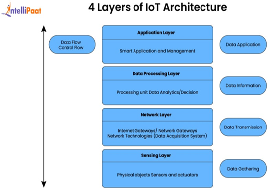
The architecture of a DAS varies mainly with respect to complexity, cost, scale, and required response time. Generally, as illustrated in Figure 1, the system comprises four core layers.
Figure 1. Layers of Internet of Things (IoT) architecture [24]
The sensor layer forms the foundation of the system and consists of physical sensing devices such as temperature and humidity sensors (e.g., DHT22), electrical conductivity and pH probes, and light sensors that directly capture environmental and soil conditions. Data from these sensors is then gathered by the data collection layer, which relies on microcontrollers or data loggers such as Arduino, ESP32, or Raspberry Pi to acquire, digitize, and organize the measurements. Once collected, the processing layer handles local or edge-level computation, where raw data may be filtered, aggregated, and analyzed to support basic decision-making before transmission. Finally, the communication layer enables the exchange of information between devices and external platforms using protocols and technologies such as MQTT, Hypertext Transfer Protocol (HTTP), LoRa, Wi-Fi, or ZigBee, ensuring reliable data flow to cloud services or user applications.
3.1.1 Manual vs. automated
In early greenhouse monitoring operations, manual data- logger methods were applied; growers would often visually inspect analog instruments or use hand-held sensors. Manual data logging is laborious, prone to error, and lacks good time resolution [25].
On the contrary, the automated DAS constantly acquire and record data with minimal human involvement using microcontroller-based systems. Table 1 contrasts manual and automated acquisition: automated systems deliver higher accuracy, high-frequency sampling, and immediate algorithmic control at far lower labor. For example, automated irrigation based on real-time soil moisture readings substantially improves water-use efficiency [26].
Studies report yield improvements of 15–30% when transitioning from manual to automated greenhouse monitoring due to improved climate stability and timely interventions.
Table 1. Manual vs. automated data acquisition systems (DASs) comparison
|
Aspect |
Manual DAS |
Automated DAS |
|
Data frequency |
Low (daily/weekly) |
High (seconds-minutes) |
|
Accuracy |
Operator-dependent |
Sensor-limited, consistent |
|
Labor requirement |
High |
Low |
|
Real-time control |
Not possible |
Enabled |
3.1.2 Wired versus wireless
In wired systems, data transmission can be carried out via RS-232, RS-485, or Ethernet cables. They are immune to electromagnetic interference and are suitable for static installations. Nevertheless, they suffer from limited scalability with installation difficulties and high maintenance in unfavorable conditions.
Wireless DAS employ protocols that include ZigBee, Wi-Fi, LoRaWAN, or Bluetooth Low Energy (BLE). These wireless systems provide modularity and scalability, particularly for large scale undertakings and modular greenhouses. Wireless DAS reduce installation cost and promote remote monitoring through cloud platforms [27]. LoRa provides long range, low power communication, which is well suited to agricultural ap- plications [28]. Table 2 compares the two-options wireless adding modularity, scalability, and remote monitoring, wired offering immunity to interference for static installations.
Table 2. Wired vs. wireless data acquisition systems (DASs) comparison
|
Criterion |
Wired DAS |
Wireless DAS |
|
Reliability |
High (low packet loss) |
Medium-High (environment-dependent) |
|
Installation cost |
High |
Low-Medium |
|
Scalability |
Limited |
High |
|
Susceptibility to noise |
Low |
Medium |
|
Maintenance |
Physical wear |
Battery replacement |
Validated findings:
•Wired RS485 systems show <1% data loss in humid greenhouse environments [29].
•Wireless LoRa-based DAS reduce installation cost by up to 40%, but introduce latency unsuitable for fast control loops [18].
3.1.3 Stand-alone vs. networked
A stand-alone DAS carries out all data logging and analysis locally without communicating with any external entity. Such systems are helpful in remote locations or research setups where internet connectivity is spotty. Through SD cards or local databases, data is stored and periodically retrieved.
Networked DAS are viewed as part of a wider cyber-physical system that generally connects to the Internet or local servers. Table 3 sets stand-alone against networked DAS, the latter adding remote access, cloud storage, real-time dashboards, and machine-learning support. These cloud-connected DAS provide predictive analytics and decision support tools vital to modern precision agriculture.
Table 3. Standalone vs. networked data acquisition systems (DASs) comparison
|
Feature |
Stand-Alone DAS |
Networked DAS |
|
Connectivity |
None / Local |
IoT-enabled |
|
Data storage |
Local |
Edge/Cloud |
|
Scalability |
Low |
High |
|
AI integration |
Limited |
Extensive |
|
Remote access |
Not available |
Fully supported |
The enhancement of edge computing in networked DAS allows preliminary processing at the sensor node, therefore, diminishing latency and bandwidth usage, enabling faster action response [30].
Validated findings:
•Networked systems enable:
•Multi-zone climate optimization
•Cross-greenhouse analytics
Predictive control using AI models
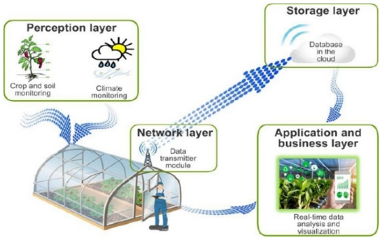
Field studies report 20-35% water and fertilizer savings in networked DAS compared to stand-alone controllers [19]. Figure 2 lays out the general IoT architecture underlying these greenhouse deployments.
Figure 2. Internet of Things (IoT) general architecture for greenhouse applications
3.2 Core components
A DAS operates with efficiencies and powers relying heavily on the choice of an arrangement of these major portions. It has four core layers containing building blocks which are sensors, computational units, and communication protocols. Each performing a very concrete obligation in the realization of environmental and agronomic data acquisition from the field to platforms for analysis [31].
3.2.1 Sensors
Sensors form the foundation of any DAS, as they provide the essential measurements required for monitoring and controlling agricultural environments. They can be broadly categorized into environmental sensors, soil sensors, and plant-specific sensors.
Environmental sensors. Environmental sensors capture the surrounding atmospheric conditions that directly influence plant growth and the prevalence of pests and diseases. For instance, temperature and humidity sensors such as the DHT22 and SHT31 are widely deployed due to their low cost and reliability. Light sensors, such as the BH1750 and TSL2561, are commonly used to measure light intensity, while BMP280 and BME680 sensors provide additional measurements such as barometric pressure, air quality, and volatile organic compounds. Monitoring these parameters allows precise climate control in greenhouses, including heating, ventilation, and pest management strategies.
•Temperature and humidity: DHT22, SHT31, SHT35.
•Light intensity: BH1750, TSL2561.
•Air quality/pressure: BME680, BMP280.
Soil sensors. Soil sensors provide critical insights into the underground growing medium, ensuring optimized irrigation and fertilization management. The most widely used devices include the Capacitive Soil Moisture Sensor v1.2, which measures volumetric water content without corrosion issues, and electrical conductivity (EC) sensors such as the Decagon 5TE and WET150, which measure EC, moisture, and temperature simultaneously. pH probes (e.g., Atlas Scientific pH Sensor) are widely used for soil acidity monitoring, while advanced nutrient sensors such as Ion-Selective Electrodes (ISE) are employed for detecting nitrogen, phosphorus, and potassium (NPK) concentrations.
•Moisture: Capacitive Soil Moisture Sensor v1.2, Decagon EC-5.
•Electrical Conductivity (EC): Decagon 5TE, WET150. pH: Atlas Scientific pH Sensor.
•Nutrient Sensors (NPK): Ion-Selective Electrodes (ISE).
Plant-specific sensors. Plant-specific sensors directly assess crop physiological status and health. Optical sensors are among the most widely applied in this category. For example, chlorophyll meters such as the SPAD-502 Plus are used to estimate leaf chlorophyll con- tent, providing insights into plant nitrogen status. Multispectral and hyperspectral imaging sensors, including Green Seeker and UAV-mounted Normalized Difference Vegetation Index (NDVI) cameras, enable large-scale monitoring of crop vigor through vegetation indices such as the NDVI. Fluorescence-based systems, such as PAM fluorometers, are also employed to evaluate photosynthetic efficiency.
•Chlorophyll Content: SPAD-502 Plus.
•Vegetation Indices: Green Seeker, UAV NDVI cameras.
•Fluorescence: PAM fluorometers.
Long-term usability for these sensors calls for considerations pertaining to environmental tolerance, drift behavior, and maintenance requirements when in a humid, dusty, or saline setting.
3.2.2 Microcontrollers
Microcontrollers are the processing core of DAS setups. They interpret raw sensor readings, apply local logic (such as thresholds or edge computing algorithms), and oversee data transmission. Typical options found in agricultural settings include:
•Arduino boards (like the Uno and Nano) are perfect for simple sensing applications where simplicity and community support are essential.
•ESP32/ESP8266 modules integrate Wi-Fi or Bluetooth and advanced power saving modes for battery-operated IoT devices.
•Raspberry Pi systems have higher computational power and are used in image processing databases or local AI model operation [32].
The ultimate choice depends on the project at hand, either simple data logging or complex on-site analytics.
3.2.3 Communication protocols
Immediately after processing, the next task is to transmit the sensor data to the external systems. The means of communication depends on the distance, energy constraints, and data frequency. Some of the important protocols are:
MQTT Protocol. The MQTT is an open-source and lightweight communication protocol specifically designed for low-bandwidth, high-latency, and resource- constrained applications. It has become one of the most widely adopted protocols in IoT ecosystems, including smart greenhouse and precision agriculture deployments.
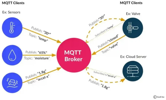
Unlike traditional client-server models, MQTT follows a publish-subscribe communication paradigm, where devices (clients) publish messages to specific topics, and other devices subscribe to those topics to receive the data. This is mediated by a central component known as the broker. Popular brokers such as Eclipse Mosquitto and HiveMQ are often deployed in agricultural IoT systems due to their scalability and reliability. The broker decouples publishers from subscribers, thereby reducing communication overhead and improving system flexibility.
Figure 3 shows how MQTT's publish–subscribe model links publishers and subscribers through a central broker. The publisher is a client that is supposed to send data to the network, such as the ESP32 sending soil moisture readings. The messages are received by a central broker that acts as an intermediate server, which takes in the incoming data and forwards them to all interested parties. A typical example is the Mosquito broker, which is either run locally or in the cloud. The subscriber is a client on the receiving end listening to particular topics to obtain the published data, which could be, say, a mobile application showing the real-time humidity values.
Figure 3. Message queuing telemetry transport (MQTT) clients [38]
Corresponding to the various needs of applications, MQTT defines three different quality levels of service (QoS), which determine signaling and delivery reliability of messages. QoS 0 is at best-effort with no acknowledgments so that message delivery is useful for noncritical data, allowing for an occasional loss. QoS 1 guarantees message at least once delivery but presumably will cause duplicate messages, while QoS 2 is the reliable way of defining on time delivery with the cost of higher communication overhead. The whole range of QoS options enables system designers to make compromises between redundancy and bandwidth efficiency, which is especially important in agricultural environments with often unstable or intermittent network accessibility.
One of the main advantages of MQTT is that it is extremely lightweight, making it particularly suitable for resource- constrained devices such as Arduino and ESP32 [33]. Its efficiency stems from the fact that its message header is only 2 bytes, ensuring minimal overhead and reduced bandwidth consumption [34]. Moreover, MQTT supports bi-directional communication, which enables not only sensor data monitoring but also remote actuation of devices, a key requirement in modern IoT and smart agriculture systems [35]. Another strength is its scalability: MQTT can operate effectively from just a few devices to thousands of interconnected nodes without significant degradation in performance [36].
Despite these benefits, MQTT also has some limitations. A major drawback is its reliance on a broker to manage communication, which introduces a single point of failure in the system. Furthermore, MQTT lacks built-in encryption and security mechanisms; security is usually enforced through the integration of TLS/SSL, which can be resource-intensive for constrained devices [37]. Finally, while MQTT is highly efficient for lightweight messaging, it is not optimized for very high- throughput or real-time streaming applications when compared to alternatives such as WebSocket or AMQP [37].
LoRaWAN Protocol. LoRaWAN is a communication protocol specifically designed for low-power, long- range wireless IoT applications [39]. It is built on top of the Long Range modulation technique, which uses Chirp Spread Spectrum (CSS) modulation to achieve reliable data transmission over distances of up to 15 km in rural areas while consuming minimal energy [40]. These features make LoRaWAN particularly well suited for large-scale smart agriculture and agribusiness applications where traditional connectivity options (e.g., Wi-Fi or cellular) are either unavailable or cost prohibitive.
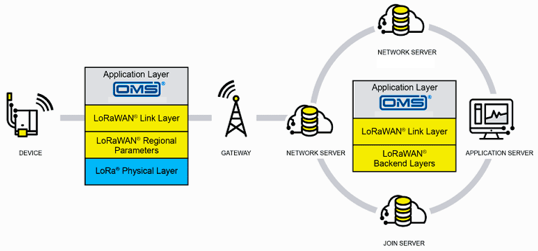
LoRaWAN operates in unlicensed Industrial, Scientific, and Medical (ISM) frequency bands, typically 868 MHz in Europe, 915 MHz in North America, and 433 MHz in parts of Asia, making it a cost-effective solution for IoT deployments. Its star-of-stars topology allows end devices to communicate with gateways, which then forward data to a central network server, ensuring simplified and scalable system design.
Figure 4 sets out the LoRaWAN architecture and its four components end devices, gateways, the network server, and the application server. The End Devices are typically battery-powered sensor nodes such as soil moisture sensors or weather stations that send data at intervals. The devices communicate with the Gateways, which relay the received LoRa-modulated signals to the Network Server over IP-based backhaul connections, such as Ethernet, Wi-Fi, or cellular networks. The Network Server is at the heart of the system with responsibility for managing the connected devices, filtering duplicate packets, and enforcing security mechanisms. The Application Server receives the processed sensor data from the Network Server and presents it to the end user applications for visualization, decision-making, and actuation.
Figure 4. Architecture of a network implementing the Long Range Wide Area Network (LoRaWAN) protocol [41]
LoRaWAN defines three classes of devices in order to cater to different power and communication requirements. Class A devices are the most power-limited; they briefly open their receive windows only after having transmitted their data. This makes class A devices suitable for sensors having a long battery life requirement. Class B devices have scheduled receive windows added for more downlink communication. Class C devices, however, keep their receivers open most of the time, thereby consuming more power and incurring less delay-more beneficial for actuation-oriented applications. The main advantages of LoRaWAN are its long communication range and ultra-low power consumption, allowing end devices to operate on batteries for up to 10 years. It also supports large-scale deployments, with a single gateway capable of handling thousands of nodes, making it highly suitable for monitoring extensive agricultural fields. Adaptive data rate mechanisms further optimize communication efficiency and battery life by adjusting transmission parameters dynamically [40]. Moreover, LoRaWAN incorporates security at both the network and application layers using AES-128 encryption, ensuring data integrity and confidentiality.
However, LoRaWAN also has notable limitations. Its data rates are relatively low (ranging from 0.3 kbps to 50 kbps), restricting it to small, infrequent sensor transmissions rather than bandwidth-intensive applications. It can also suffer from increased latency, particularly in Class A devices, which is unsuitable for time-critical control operations. Additionally, since LoRaWAN operates in unlicensed spectrum, it is subject to duty-cycle restrictions and interference, which may cause network congestion in densely deployed areas. These tradeoffs make LoRaWAN ideal for large-scale, low-data-rate sensing in agriculture, but less appropriate for applications requiring real time communication.
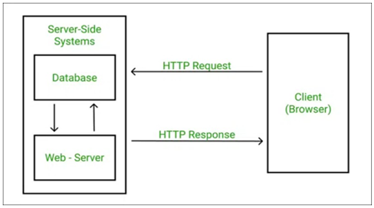
HTTP Protocol. The HTTP is one of the most established and universally adopted communication protocols in Internet-based systems and continues to play an important role in IoT deployments, including smart greenhouse applications. Despite being comparatively more resource-intensive than lightweight protocols such as MQTT or CoAP, HTTP remains highly relevant due to its seamless integration with cloud infrastructures, RESTful APIs, and visualization dashboards [42, 43]. Its ubiquity makes it particularly advantageous in Wi-Fi-enabled greenhouse environments, where sensor nodes and microcontrollers (e.g., ESP32 or Raspberry Pi) can transmit data directly to web servers or cloud platforms without re- quiring additional middleware.
HTTP is based on a client-server communication model, in which IoT devices act as clients that initiate requests (e.g., GET, POST, PUT) to servers that process and store the data. This paradigm enables real-time greenhouse sensor readings, such as temperature, humidity, and soil moisture, to be uploaded to cloud dashboards for monitoring, visualization, and analytics. The standardized request methods provide an efficient structure for interaction with web services, making HTTP especially suitable for integration with existing data management and decision-support platforms.
In the context of smart agriculture and green- house IoT systems, an HTTP-based architecture typically includes three primary elements: the client, which corresponds to IoT devices responsible for sensing and transmitting environ- mental data; the server, often deployed on cloud infrastructures such as Amazon Web Services (AWS) IoT Core or Microsoft Azure IoT Hub, where data is aggregated and processed; and the user interface, which can take the form of mobile or web-based dashboards that support real time decision making [42]. This architecture leverages the maturity of HTTP and its compatibility with web technologies to ensure system scalability and accessibility.
Figure 5 traces HTTP's synchronous request–response exchange: unlike MQTT's publish-subscribe model, the server replies only when the client queries it. While this approach facilitates straightforward integration with web services, it also results in higher latency and energy consumption in scenarios requiring frequent or continuous data exchange [44]. In greenhouse environments where sensors generate frequent updates, this overhead can re- duce efficiency compared to event-driven protocols.
Figure 5. Hypertext transfer protocol (HTTP) request/response protocol
The main advantage of HTTP lies in its universality: it is widely supported across all devices, operating systems, and cloud platforms, thereby reducing complexity in the design and deployment of greenhouse IoT systems. HTTP also offers robust interoperability with web applications and APIs, simplifying integration with third-party services and decision support tools. Furthermore, the maturity of HTTP ensures stability, reliability, and security mechanisms through HTTPS, which protects sensitive agricultural data transmitted over public net- works [45].
On the other hand, HTTP presents several challenges for IoT applications in agriculture. Its relatively high bandwidth consumption, due to large header sizes, is inefficient in low power or low-bandwidth environments. The synchronous communication model also makes HTTP less suitable for real-time control applications, where protocols such as MQTT or CoAP provide better responsiveness and energy efficiency. Additionally, while HTTPS enables secure communication, the computational overhead of TLS/SSL encryption can be taxing for microcontrollers with constrained resources, thus limiting scalability in resource-limited deployments [46].
For these reasons, HTTP is most often adopted in hybrid greenhouse communication architectures, where it complements lightweight protocols: frequent sensor updates are typically handled via MQTT or LoRaWAN, while HTTP is employed for higher-level operations such as device configuration, external API integration, or data visualization on web-based dashboards.
No single protocol is optimal: as Table 4 shows, MQTT, LoRaWAN, Wi-Fi, and BLE each trade off range, energy, and throughput differently. MQTT minimizes overhead for frequent, small telemetry but presumes reliable connectivity and a broker. LoRaWAN reaches kilometers at milliwatt power, but its low data rate and duty-cycle limits rule out image or high-frequency streams. Wi-Fi and BLE offer higher bandwidth over short ranges at greater energy cost. The choice therefore depends on the deployment scenario: dense, powered, single-structure greenhouses favor MQTT over Wi-Fi, sparse off-grid or multi-hectare sites favor LoRaWAN, and image-heavy phenotyping pipelines require higher-bandwidth links or local edge processing to avoid the network entirely.
Table 4. Communication protocols comparaison
|
Technology |
Typical Range |
Data Rate |
Power Consumption |
Network Topology |
Key Strengths |
Main Limitations |
Typical Use in Smart Agriculture |
|
Wi-Fi |
50–100 m |
High (Mbps) |
High |
Star |
High bandwidth, low latency, easy integration with IP networks |
High energy use, limited range, poor scalability for sensors |
Cameras, gateways, edge AI devices inside greenhouses |
|
Bluetooth LE |
10–30 m |
Low-Moderate |
Very Low |
Star |
Ultra-low power, simple pairing, supported by smartphones |
Very short range, not suitable for continuous monitoring |
Wearable sensors, handheld diagnostics, device configuration |
|
Zigbee |
10–100 m (mesh) |
Low |
Low |
Mesh |
Scalable, low power, self-healing networks |
Interference in 2.4 GHz band, moderate data rate |
Dense greenhouse sensor networks |
|
Long Range Wide Area Network (LoRaWAN) |
2–15 km |
Very Low |
Ultra-Low |
Star |
Long range, years of battery life, license-free |
High latency, low throughput, not real-time |
Distributed field sensors, environmental monitoring |
|
Narrowband Internet of Things |
>10 km (cellular) |
Low |
Low-Moderate |
Cellular |
Wide coverage, reliable quality levels of service (QoS), good penetration |
Subscription cost, operator dependency, higher latency |
Large-scale farms, remote monitoring, national deployments |
3.2.4 Data management
With smart agricultural systems producing immense quantities of data, data management not only takes on a critical role in real-time control but also long-term analysis, optimization, and traceability. Raw data must be analyzed, but it must also be efficiently processed, stored, and retrieved to squeeze out value. This section will explore, in depth, the three pillars of modern data management for greenhouse systems: edge computing, cloud storage, and database design.
Edge processing. Edge processing entails analyzing and interpreting sensor data at or near the source, almost always on microcontrollers, embedded systems (Raspberry Pi, etc.), or edge gateways. By this method, latency, bandwidth consumption, and reliance on a constant internet connection are much lessened [47].
In a greenhouse, an edge-enabled microcontroller might evaluate temperature and humidity readings every few seconds locally and turn on a cooling fan or irrigation system when exceeded thresholds have been set. This will enable real-time control fast into remote areas that may not have access to the cloud. Furthermore, preprocessing at the edge-such as noise filtering, thresholding, or extracting trends-decreases the volume of data sent over to the cloud, making for a more efficient and hardened system.
Advanced edge systems can support light machine-learning models such as TensorFlow Lite or Tiny machine learning, for detecting anomalies or predicting events, such as a pest outbreak, which provides more autonomy at the device level [47].
Cloud storage. Cloud computing complements edge processing by providing massive on-demand storage and access to standardized environments with the computational power required to run complex analytics. Platforms such as AWS, Microsoft Azure, and Google cloud.
In the greenhouse context, cloud storage serves multiple purposes:
•Historical Data Logging: Enables tracking of growing conditions and system performance over extended periods, including weeks, seasons, or even years.
•Multi-user Access: Multiple stakeholders such as farmers, agronomists, and researchers can remotely monitor and collaborate using the same data.
•Backup and Redundancy: Ensures data reliability by duplicating records on geographically distributed servers in the event of local device failure.
Additionally, cloud platforms can integrate with third-party applications such as weather forecasting APIs, agricultural databases, and market prediction models, further enhancing data-driven decision-making.
3.3 Database design
Database design. The effectiveness of the database design is, here, the pillar to allow timely storage, retrieval, and analysis of data. Most data flowing into the greenhouse environment is of time-series nature, acquired through sensors at regular intervals. Influx DB, Time scale DB, and OpenTSDB are some examples of time- series databases (TSDBs) that are best suited for this type of structured temporal data [48]. They offer high throughput in writing and instantaneous querying of trends, averages, and thresholds over time.
A well-designed agricultural database would encompass:
•Sensor Metadata: Location, type, and calibration information.
•Data Schema: Usually follows a template like (times- tamp, sensor ID, parameter, value, unit).
•Indexing: For a fast retrieval based on sensor location, type, or time range.
Hybrid relations seem to have been adopted by some systems; for example, MySQL or PostgreSQL might hold user data, configurations, and alerts, while NoSQL or TSDB might be in charge of the continuous flow of sensor inputs. Overall, normalization helps remove data redundancy, increases storage optimization, and hence enhances the scalability of the system. Finally, the synergy of edge computing, cloud services, and an appropriately designed database ensures that smart green- house systems can react, prophesy, and be prepared for expansion.
Effective climate management begins with the four environmental variables that most directly govern plant growth: temperature, humidity, light, and CO₂.
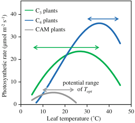
The temperature is actually what mostly affects plant metabolism rates. Temperature optimal exist for enzymatic activity, photosynthesis, respiration, and membrane fluidity. Figure 6 plots the temperature response of C3 versus C4 photosynthesis, with C3 crops (lettuce, spinach) peaking at 18–25 ℃ and C4 crops (tomato, maize) tolerating up to 30 ℃ [49].
Figure 6. C3 vs. C4 photosynthesis temperature response curve [49]
Diurnal and nocturnal temperature differences (DIF) are manipulated in greenhouses as a technique to regulate the morphology of plants. A positive DIF, where day temperature is higher than night, favors stem elongation, whereas a negative DIF leads to a shortening of internodal length, thus favoring compact growth [50].
Thermal screens form part of the greenhouse heating systems (boilers, hot water pipes), cooling systems (evaporative cooling, fans, misting), and temperature maintenance within the crop comfort zone [51]. Thermal mapping can be done using thermographic imaging and distributed temperature sensors.
Humidity affects transpiration, nutrient uptake, and the development of plant pathogens. Relative Humidity (RH) and Vapor Pressure Deficit (VPD) are used for measurements of moisture levels in the air. Low RH results in greater water vapor loss, increasing the likelihood of water stress and nutrient imbalance. High RH lowers transpiration and enhances disease incidence, particularly *Botrytis* and powdery mildew [52].
Generally, 60–80% RH and 0.5–1.2 kPa of VPD are considered optimal [53]. Automated fogging, dehumidifiers, and vent actuation are currently used to regulate moisture levels in modern systems. Control of VPD is becoming standardized in precision greenhouse farming today [54].
Light provides photosynthetic energy and has characteristics such as intensity (PPFD, µmol·m−2·s−1), spectrum (wave- length), and photoperiod (duration). Different wavelengths af- fect various physiological processes in plants:
•Blue light (400–500 nm): compact growth and stomatal opening.
•Red light (600–700 nm): stem elongation and seed germination.
•Far-red light (700–750 nm): shade avoidance and flowering signals.
LED lighting systems allow dynamic spectral manipulation to optimize photosynthesis and morphogenesis [54]. In artificial light contexts, low-light greenhouses combine their lighting with sensors and algorithms to meet the Daily Light Integral of each crop [54].
Photosynthesis uses CO2 as its carbon source. Under con- trolled temperature and light, increasing CO2 concentrations from ambient (400 ppm) to 800–1200 ppm can significantly enhance biomass accumulation, especially in fast-growing green- house crops like tomato and cucumber [55].
This section moves from classical machine learning toward deep and reinforcement learning, emphasizing where each is justified by data availability and task type. Due to the increasing demand for the sustainable course of agriculture, an impetus is created for introducing a precision farming ideology that uses machine learning models for crop management from sensor data analysis and optimization of resource use. In smart greenhouses, real-time actionable insights obtained from interconnected sensors and predictive algorithms can identify nutrient deficiency, predict environmental change, and activate the control system, thereby enhancing yield and reducing waste [53]. This chapter would lay the foundation for coupling state-of-the-art deep learning with robust sensor networks to predict NPK deficiencies in lettuce and maintain ideal growing conditions using an intelligent IoT architecture [56].
5.1 Fundamentals of machine learning
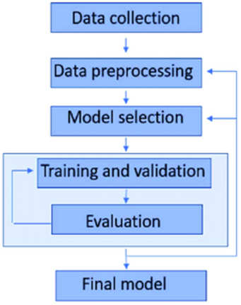
As illustrated in Figure 7, modern machine learning systems are structured as pipelines with interdependent stages: problem scoping, data collection and engineering, modeling, evaluation, and deployment [57]. From a software engineering perspective, this workflow covers the entire lifecycle of model development and constitutes one re- producible and automated methodology for the development of concrete and working machine learning applications. The pipeline structure ensures that all components are executed accordingly, thereby putting arsenal into the hands of developers and data scientists in the end-to-end development and experimentation life cycle [58]. For example, in smart agriculture, using pipelines allows machine learning algorithms such as yield prediction, regression models to be incorporated using historical data like soil quality and weather conditions to forecast parameters such as crop productivity [59]. Thus, machine learning pipelines help in the technicalities but also facilitate the actual decision- making and resource optimization in different fields.
Figure 7. Machine learning workflow diagram [60]
5.1.1 Data collection
Data collection entails acquiring raw observations (e.g., sensor readings, images, logs) and, increasingly, pairing labels via crowdsourcing or weak supervision techniques. Related recent surveys highlight developments in labeling techniques, with automatic and human-in-the-loop processes alike, to counteract bottlenecks in large-scale data acquisition, emphasizing strategies for cost-efficient acquisition of top-notch data annotation [55].
Data acquisition. Data acquisition encompasses three main strategies:
•Data discovery: Finding and accessing datasets of interest from different sources structured like relational databases, unstructured like social media streams, or coming in from a sensor network often through collaborative sites like DataHub, which supplies search, versioning, and integration tools to ease dataset discovery while guaran- teeing dataset provenance.
•Data augmentation: To enlarge artificially existing datasets through, e.g., geometric/image transformations,GAN-based sample synthesis, or rule-based perturbations, increasing diversity tremendously without any further efforts for data collection.
•Data generation: Complete data synthesis with the help of simulators or procedural models (e.g., rendering engines for computer vision), which allows the controlled exploration of corner-case scenarios very rarely or expensive to capture in the real world.
Crowdsourcing. Crowdsourcing distributes the labeling tasks to an online labor pool in large numbers, then uses redundancy, aggregation, and active learning to keep the quality while scaling. Key platforms include:
•Revolt: Executes repeated labeling and smart label aggregation; eliminates or down-weights bad contributions to increase final label quality.
•CrowdER: Its specialty is entity resolution-using human judgment to merge records that identify the same real- world entity and hence, disambiguate records from the automated perspective.
•Qurk: Brings crowdsourcing into database operations. It provides interfaces where users can hand out tasks and automatically ensures there is enough redundancy and consensus on what the correct labels are.
Weak supervision. Weak supervision methods produce large volumes of labels through programmatic rules or noisy sources, and then statistically model to refine the labels:
•Data programming (e.g., Snorkel): The user writes a set of labeling functions which are heuristics, regex patterns, or weak classifiers that label data with noisy labels. Then a generative model estimates the accuracy and correlation of these functions to produce probabilistic labels, which are subsequently used in a downstream discriminative model for robust training from large datasets.
•Fact extraction and distant supervision: Systems like Never-Ending Language Learning (NELL) and Knowledge Vault crawl unstructured web text, extracting entity- relation facts. These facts become seed labels with which to annotate large corpora automatically (distant supervision), trading noise for scale while providing useful initial annotations.
Hence, the more these kinds of acquisition and labeling strategies become combined, the more practitioners could create large-scale datasets enriched with annotations, even if they lack resources for this undertaking. This, in turn, gives machine learning a robust foothold applying generalization.
5.1.2 Data preprocessing
Preprocessing is a set of crucial tasks conducted on raw data to convert it into the input format while considering the missing values, conversion of features, and elimination of outlying observations. These operations reduce noise and bias, lowering errors and increasing generalization.
Yandrapalli [61] proposed an automated framework for data quality assessment through a bouquet of statistical and machine learning techniques. This framework combined irrespective outlier detection methods: Tukey’s IQR, which had the highest sensitivity towards extreme values, Isolation Forest (IF), being a tree-based anomaly-detector, and DBSCAN, being a density-based clustering algorithm. Post-data cleansing, they were then used for training models such as logistic regression, KNN, and Naive Bayes, which displayed an improved performance.
The study evokes the relevance of structured autoscaling be- fore learning and hence established a privileged position for automated governance frameworks in machine learning pipelines [62].
5.1.3 Modeling
In modeling, one selects algorithms such as deep networks, ensemble methods, or support vector machines and trains them to memorize some patterns for prediction. Within the purview of smart agriculture, the most recent research highlights employing artificial intelligence, big data analytics, and remote sensing toward predictive modeling in crop health monitoring, irrigation optimization, and pest management. These modeling techniques become instrumental in enabling the data-driven decision- making and improving efficiency and sustainability in agricultural practices [63].
5.1.4 Evaluation
In smart agriculture and smart greenhouse systems, it is crucial to check on machine learning performances to be able to as- certain their reliability and adaptability towards real world variability. Models ought to perform beyond just the simple classification with respect to other environmental conditions and sensor discrepancies
Classification metrics
•Accuracy: Measures the proportion of correctly predicted instances out of the total number of predictions. While intuitive, it may be misleading when class distributions are imbalanced (for example nutrient deficiency is rare).
Accuracy $=\frac{T P+T N}{T P+T N+F P+F N}$ (2)
Precision and Recall
•Precision: Evaluates the proportion of true positives among all predicted positives. Crucial when false positives are costly
Precision $=\frac{T P}{T P+E P}$ (3)
•Recall (Sensitivity): Measures the proportion of true positives identified among all actual positives. Important when missing a positive case (e.g., nutrient deficiency) has serious implications
Recall $=\frac{T P}{T P+F N}$ (4)
•F1-Score: The harmonic mean of precision and recall. Balances both false positives and false negatives, making it especially useful for imbalanced classification tasks such as nutrient deficiency detection.
$F 1=\frac{2 * \text { Precision} * \text { Recall}}{\text { Precision}+ \text { Recall}}$ (5)
•Root Mean Squared Error (RMSE): A widely used metric in regression problems. It penalizes larger errors more than smaller ones, making it suitable for yield prediction or continuous soil nutrient monitoring.
$R M S E=\sqrt{\frac{1}{n} \sum_{i=1}^n\left(y_i-\hat{y}_i\right)^2}$ (6)
•Mean Absolute Error (MAE): Average absolute difference between predicted and actual values. Robust to outliers
$M A E=\frac{1}{n} \sum_{i=1}^n\left|y_i-\hat{y}_i\right|$ (7)
•R² (Coefficient of Determination): Indicates the pro- portion of variance in the dependent variable that is predictable from the independent variables. Useful in evaluating environmental forecasting models.
$R^2=1-\frac{\sum_{i=1}^n\left(y_i-\hat{y}_i\right)^2}{\sum_{i=1}^n\left(y_i-\bar{y}_{\imath}\right)^2}$ (8)
•Receiver Operating Characteristic–Area Under Curve (ROC-AUC): Measures the ability of a classifier to distinguish between classes, independent of decision threshold.
$\int_0^1 T P R(F P R) d(F P R)$ (9)
$T P R=\frac{T P}{T P+F N}, \quad F P R=\frac{F P}{F P+T N}$ (10)
Figure 8. Confusion matrix [60]
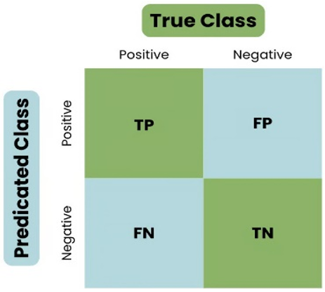
The confusion matrix is a fundamental tool for visualizing the performance of classification models, especially in multi-class or imbalanced scenarios common in smart agriculture. As illustrated in Figure 8 the counts of true positive (TP), true negative (TN), false positive (FP), and false negative (FN) predictions, allowing a detailed error analysis. By examining the confusion matrix, practitioners can identify which classes the model confuses most often and tailor improvements accordingly. For example, in nutrient deficiency detection, understanding whether the model tends to miss deficient cases (high FN) or wrongly flags healthy plants (high FP) is critical for practical deployment.
5.1.5 Statistical comparison tests
Table 5 lists the statistical tests used to compare models when differences are subtle.
Table 5. Statistical tests for model comparison
|
Test |
Purpose |
|
McNemar’s test |
Compares paired classification outcomes; ideal for bi- nary models on the same dataset. |
|
DeLong’s test |
Compares two AUCs from ROC curves statistically. |
|
Wilcoxon signed-rank |
Non-parametric test for comparing two models over multiple runs/folds. |
|
F-test |
Compares model variances; assumes normality. |
|
Bartlett’s and Levene’s tests |
Assess equality of variances; more robust to deviations from normality. |
To assess systematically on performance, one needs to set up notation or metrics for both classification and regression tasks. According to the previous study [63], in a 2024 Frontiers in Bioinformatics re- view, one must be wary of overly relying on single metrics, such as accuracy, especially when imbalanced sets or non-stationary conditions plague the data [64]. It is instead advised that stratified cross-validation and domain-dependent metrics, tailored in the agricultural context, be used, such as those sensitive to the false negative detection of nitrogen deficiency. Similarly, Rainio et al. [62] evaluates such evaluation strategies across crop diagnostics and underscores the need for real-field testing beyond the lab to assess real robustness and transferability.
Evaluation protocols typically integrate k-fold cross- validation, domain-specific robustness tests, and sensitivity analyses to simulate deployment variability, and thus they as- sure that the models are not only statistically valid but agronomically viable.
5.1.6 Deployment
Deployment involves putting the validated model into a live production environment for real-time inference. There are of- ten prerequisites like containerizing, orchestrating APIs, and setting up continuous monitoring infrastructure to ensure scalability and reliability. According to the study [65], there are three major phases in deployment: integration, monitoring, and updating. Integration often throws up challenges in configuration debt, tangled pipelines, and lack of collaboration between data science and engineering teams. Monitoring comes with machine learning-specific metrics like data drift, bias, and prediction performance, which are much harder to either define or act upon as compared to traditional software logs. Updating models in response to concept drift remains a weak point in many machine learning systems, with few organizations supporting seamless retraining and rollback.
In contrast, the study [66] proposed a structured framework to assess deploy ability through risk analysis wherein operational scenarios are defined with potential damage estimated, and Key Risk Indicators (KRIs) computed by weighting these risks by likelihood. The framework explicitly measures robustness to input corruptions, distributional shifts, and adversarial perturbations, providing a standardized way to compare deploy ability across systems.
The combined insights from these two studies reveal both the practical and theoretical underpinnings of machine learning deployment. On the practical side, containerization (Docker, Kubernetes), as well as API orchestration, are essential for modularizing model infrastructure and supporting real-time inference. However, as studied by Paleyes et al. [64], those are not a silver bullet and must be integrated with careful attention to system architecture and team workflow. On the theoretical side, the deploy ability framework by Heymann et al. [66] enabled organizations to quantify the risk associated with deployment decisions and infrastructure choices, thereby formalizing the assessment of operational robustness.
5.2 Learning paradigms
Learning paradigms stand apart from each other in terms of the availability of training feedback. Historically, three methods were considered the core of complete machine learning: supervised learning, unsupervised learning, and reinforcement learning [67]. Recently, however, semi-supervised methods have gained prominence in addressing the gap between labeled and unlabeled data. Below, each of these paradigms is explored along with examples, methods, and challenges they pose.
5.2.1 Supervised learning
In supervised learning, a model f is trained to associate given inputs-interpreted as x-with the correct outputs or answers, seen as y, provided by a labeled dataset {(xi, yi)}. Hence, supervised learning opens the doors to implementing classical algorithms, such as the support vector machine (SVM), decision trees, and random forests, as well as newer deep architectures like convolutional neural networks (CNNs) for images [68].
Supervised learning in smart greenhouses. In controlled agriculture, supervised learning is usually associated with the tackling of crop disease recognition, yield prediction, and environmental control optimization.
Classification. Identifying plant health status (healthy vs. diseased), detecting pest presence, or categorizing crop maturity levels from sensor or image data.
Regression. Predicting continuous variables such as soil moisture, nutrient concentration, or expected yield based on sensor readings and historical records.
Supervised learning algorithms give highly accurate and explainable predictions when an ad- equate amount of labeled data is present. Thus, such methods work well for decision-making in irrigation scheduling, fertilization, and disease detection. However, the major challenge lies in the need for huge amounts of annotated agricultural data. Such data collection is often expensive and lengthy; for in- stance, crop disease diagnosis often requires the input of experienced pathologists. Furthermore, such models can suffer from overfitting in cases of imbalanced datasets (e.g., more healthy samples than diseased), thus limiting their generalization to actual farming conditions.
5.2.2 Unsupervised learning
Unsupervised methods try to find structure in unlabeled data {xi} by discovering patterns like clusters or low-dimensional manifolds [68].
Key Methods:
•Clustering (e.g., k-means, hierarchical): Groups similar samples without labels.
•Dimensionality Reduction (e.g., PCA, t-SNE): Finds compact representations that preserve variance or neighborhood relationships.
Advanced Example: introduce SwAV, which simultaneously clusters multiple augmented views of each image and enforces consistency between their assignments, eliminating the need for costly pairwise comparisons and large memory banks while achieving 75.3% top-1 accuracy on ImageNet with ResNet-50 [69].
Unsupervised learning is crucial for pretraining representations that can be fine-tuned with limited labels, especially in domains where annotations are scarce.
5.2.3 Semi-supervised learning
Semi-supervised learning (SSL) combines a small labeled set with a larger pool of unlabeled data to boost performance when labels are expensive. Emmert-Streib & Dehmer classify SSL as one of the” modern” paradigms that extend the classical three. Oliveira and Berton provide a detailed taxonomy of SSL methods addressing class imbalance, organizing techniques into eight categories: balancing, graph based, loss based, self-training, ensemble, active learning, postprocessing, and other methods [70].
Common SSL strategies. Several approaches were proposed with an intention to make the best use of the unlabeled data within the usual working arrangements of SSL. An attempt is made to summarize the most commonly used methods under the categories below:
•Self-training: A model is first trained on a rather small labeled dataset and is subsequently applied to assign pseudo- labels to unlabeled samples. An iteratively built-up training set consists of samples carrying confident predictions. Gradually this training will improve the model performance. While it is simple, it also can propagate errors if wrong labels are assigned by the model in the initial steps.
•Graph-based methods: These treat both labeled and un- labeled data points as nodes in a graph, where edges reflect the degree of similarity between instances. Labels then propagate through the graph structure consistent with the underlying assumption that samples that are similar share the same label. Such approach is particularly effective when the relational structure naturally exists in the domain, for example, in sensor networks or biological datasets.
•Loss-based regularization: Instead of just assigning labels, these modern methods tweak the loss function such that smoothness or consistency is applied over un- labeled data. For instance, entropy minimization, which pushes the model toward confident predictions, and consistency regularization, which enforces stability of pre- dictions under data perturbations. Such approaches are widely adopted in modern SSL frameworks due to their flexibility.
•Hybrid strategies: Recent work often combines the above paradigms, e.g., using self-training together with consistency losses, or integrating graph information into pseudo-labeling. These hybrid approaches aim to reduce the weaknesses of individual methods and achieve more robust performance in real-world scenarios
5.2.4 Reinforcement learning
Reinforcement learning has emerged as a powerful paradigm for sequential decision-making problems, where an agent learns by interacting with its environment. At each discrete time step $t$, the agent observes a state $s_t \in S$, selects an action $a_t \in A$, receives a scalar reward $r_t \in R$, and transitions to a new state $s_{t+1}$. The objective is to learn a policy $\pi(a \mid s)$ that maximizes the expected cumulative discounted reward.
•Markov decision process (MDP): reinforcement learning problems are often formalized as an MDP defined by the tuple $(S, A, P, R, \gamma)$, where $S$ is the state space, $A$ is the action space, $P\left(\left.s\right|^{\prime} s, a\right)$ is the transition probability, $R(s, a)$ is the reward function, and $\gamma \in[0,1]$ is the discount factor controlling the importance of future rewards.
•Objective function: The agent aims to maximize the expected return, defined as:
$J(\pi)=\mathbb{E}_\pi\left[\sum_{t=0}^{\infty} \gamma^t r_t\right]$ (11)
•Value functions: The state-value function Vπ(s) and the action-value function Qπ(s, a) quantify the expected return starting from state s or state-action pair (s, a), respectively:
$V^\pi(s)=\mathbb{E}_\pi\left[\sum_{t=0}^{\infty} \gamma^t r_t \mid S_0=s\right]$ (12)
$Q^\pi(s, a)=\mathbb{E}_\pi\left[\sum_{t=0}^{\infty} \gamma^t r_t \mid S_0=s, a_0=a\right]$ (13)
•Policy optimization: Policy-based methods adjust parameters θ of a differentiable policy πθ(a|s) to maximize J(πθ). The policy gradient theorem provides a foundation for this:
$\nabla_\theta j\left(\pi_\theta\right)=\mathbb{E}_{s, a \sim \pi_\theta}\left[\nabla_\theta \log \pi_\theta(a \mid s) \varrho^{\pi_0}(s, a)\right.$ (14)
This principle underlies modern algorithms such as REINFORCE, PPO, and A3C [71].
In recent years, DRL processes have undergone tremendous growth, mainly with respect to sample efficiency, stability, and scaling aspects. For example, off-policy techniques like SAC employ entropy regularization to reward exploration and pre- vent premature convergence [72-74]. On the other hand, model-based reinforcement learning types try to learn dynamics in order to limit the need for expensive real interactions in the real world [75]. Meta-reinforcement learning and multi-agent reinforcement learning have also been studied for real applications requiring adaptability and cooperation [76].
Reinforcement learning has been used extensively in robotics control (autonomous drones, manipulators), game playing (AlphaGo, AlphaStar), and sequential decision systems in recommendation engines, autonomous driving, and energy management. In agriculture, reinforcement learning has been employed for irrigation scheduling, greenhouse climate control, and resource allocation in dynamic environments where the reward signifies productivity or sustainability [77].
Despite its success, reinforcement learning faces several challenges when applied to real-life domains, such as smart agriculture. A major problem here is the exploration exploitation dilemma, where the agent must decide between trying new strategies to see if better payoffs can be procured and exploiting known rewarding strategies. Most reinforcement learning methods, however, tend to be sample-inefficient, meaning that they take a very long while interacting with the environment before they can provide stable performance. This is usually exacerbated by the high variance in the gradient estimates of policy optimization algorithms, making them unstable and hard to scale into complex agricultural systems.
5.3 Overfitting
It arises when a model learns noise or idiosyncratic quirks of the training set rather than the underlying distribution, thereby undermining its performance on fresh data.
5.3.1 Susceptibility of small or low-dimensional datasets
Charilaou and Battat emphasize how machine-learning models, while mostly outperforming classical regression, must nonetheless be rigorously validated, lest they over-fit on small clinical datasets (e.g., n = 146) where “naive” AUCs (trained on all data) substantially exceed cross-validated AUCs; this is evidence of over-fitting [78].
Subramanian and Simon provided simulation evidence for serious over-fitting of low-dimensional data (p ¡ n) due to weak predictor outcome relationships, advocating for either a separate test set or complete cross-validation regardless of dimensionality
5.3.2 Hyper-parameter tuning and nested cross-validation
When tuning model hyper-parameters such as network depth and regularization strength, performing k-fold cross-validation both to select hyper-parameters and to evaluate performance can itself induce bias. Charilaou and Battat suggest a nested k-fold design to remedy this situation, with an inner loop for hyperparameter search and an outer loop for final performance estimation, thus preventing optimistic performance inflation.
5.3.3 Events-per-variable considerations
In classification tasks with binary outcomes, the rule of thumb of at least ten events per predictor helps guard against over-fitting in logistic models. In small data settings, both the number of folds and stratification by outcome prevalence must be chosen carefully to ensure each training fold contains sufficient positive events. Table 6 contrasts underfitting and overfitting, the two error regimes that careful validation must guard against.
Table 6. Comparison of underfitting and overfitting [78, 79]
|
Aspect |
Underfitting |
Overfitting |
|
Training error |
High |
Low |
|
Validation error |
High |
High |
|
Model complexity |
Too low (e.g. shallow tree, few parameters) |
Too high (e.g. deep tree, excessive parameters) |
|
Root cause |
High bias; model too simple to capture signal |
High variance; model fits noise in training data |
|
Typical dataset size |
Insufficient data or overly constrained model |
Often small datasets or excessive capacity |
|
Remedies |
Increase model complexity; add features |
Regularization; more data; cross-validation |
5.4 Generalization
Generalization measures how well a model trained on one dataset performs on truly new data, reflecting its real-world utility.
5.4.1 Overconfidence and under-performance pitfalls
Aliferis and Simon survey scenarios in which overconfident models, those exhibiting high apparent accuracy on validation sets fail on new data. They outline best practices (e.g., robust validation, calibration techniques) to prevent and correct over confidence and under-confidence, underscoring that generalization is not guaranteed simply by model complexity control [80].
5.4.2 Class-dependent effects of regularization
Regularization curbs the overfitting discussed in Section 5.3, but its constraints are usually tuned to maximize average accuracy and therefore do not affect every class equally often eroding performance on the under-represented classes, which in greenhouse datasets tend to be the diseased or nutrient-deficient plants of greatest interest. Table 7 summarizes common regularization techniques and how their effects vary by class.
Table 7. Regularization techniques and their effects [80, 81]
|
Technique |
Mechanism |
Typical Effect on Classes |
|
Weight decay |
Adds an L2 penalty on large weights |
Uniform shrinkage; may underperform on minority classes |
|
Data augmentation |
Creates synthetic variants (e.g. random crops, flips) |
Improves robustness but can bias against specific classes |
|
Dropout |
Randomly zeroes network activations during training |
Reduces co-adaptation; may harm rare feature detection |
|
Early stopping |
Halts training once validation loss plateaus |
Prevents late-stage overfitting; risk of under-training |
|
Batch normalization |
Normalizes activations within minibatches |
Smoother loss surface improves generalization |
Balestriero, Bottou, and LeCun reveal that standard regularizes like data augmentation (random crops) or weight decay, tuned via cross-validation to maximize average accuracy, can disproportionately harm performance on specific classes. For example, when training a ResNet-50 on ImageNet, introducing random-crop augmentation reduces” barn spider” test accuracy from 68% to 46%, illustrating that naive regularization can introduce hidden biases in generalization [79].
5.5 Cross-validation
Cross-validation refers to performing several train/test splits in order to provide more reliable estimates at different levels of confidence regarding out-of-sample prediction performance and to guard against over-fitting.
5.5.1 Power and confidence issues in nested k-fold
Ghasemzadeh et al. [79] tested four kinds of validation methods, single holdout, k-fold, train-validation-test, and nested k-fold, on clinical voice data. Nested 10-fold cross-validation produces the highest statistical confidence (likelihood of selecting the correct features) and an unbiased estimate of accuracy; on the other hand, single-holdout models grossly overestimate performance and need maybe 50% more samples to attain the same power. Nested k-fold might yield an improvement of nearly 4 times in confidence over simpler splits [82].
5.5.2 Spatial and domain transferability
Habibi, Matsui, and Tanaka evaluate random CV, spatial CV (cluster-based), and leave-one-field-out CV for UAV-based soy- bean yield prediction. Random CV fails to capture variability beyond the training domain, while the spatially aware CV strategies are better candidates for extrapolating to new fields. Moreover, applying simple models (LASSO with recursive feature elimination) further enhances transferability, recommending spatial CV as a standard for robust, real-world yield forecasting [81].
5.5.3 K-Fold for transformer-based symbolic regression
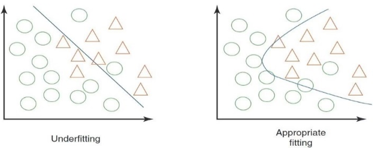
Implements 5-fold cross-validation on a transformer- based symbolic regression model trained on only 15,000 (vs. 500,000) synthetic data points. K-fold CV reduces over-fitting, improving validation loss by 53.31% relative to a standard 80/20 train/test split, and yields performance comparable to a model trained on a much larger dataset. Such findings give evidence that K-fold CV is significant for the generalization of models in data-poor environments. Figure 9 illustrates the difference between appropriate fitting and underfitting.
Figure 9. Appropriate fitting vs. underfitting illustration
Where classical machine learning depends on hand-crafted features, the deep-learning architectures examined here (CNNs for images, recurrent neural network (RNN) / long short-term memory (LSTM) networks for time series) learn representations directly from data, at the cost of larger training requirements.
6.1 convolutional neural networks for visual pattern recognition
CNNs have emerged as a powerful tool for visual pattern recognition in precision agriculture, particularly for detecting nutrient deficiencies in crops. These architectures automatically learn spatial hierarchies of features from leaf images, effectively capturing color, texture, and shape patterns indicative of NPK imbalances. Recent advances demonstrate that CNNs can achieve high classification accuracy even with limited labeled datasets when enhanced with data augmentation techniques.
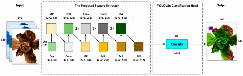
Figure 10 shows the YOLO-NPK architecture used for lettuce nutrient-deficiency classification, a model that stands out in contemporary research. According to the comparative evaluations, this Classification which achieves a top-1 accuracy of 99%, with computational performance of 9.2 G FLOPs and latency of 64.1 ms per image. These results far exceed the baseline requirements (top-1 accuracy >85%, FLOPs <10G, latency <170 ms) and performance levels of other methods, which satisfied the computational constraints but violated accuracy targets. The model’s custom-built feature extractor works particularly well in catering to the challenges of lettuce deficiency classification while still keeping the computational efficiency low enough for edge deployment.
Figure 10. Architecture of YOLO-NPK for lettuce deficiency classification [83]
This research, therefore, established a strong framework for visual nutrient deficiency detection that equally weighs accuracy and performance. The proved results give strong cues about their integration as part of a full-fledged smart farming system, with future work to be centered on deployment scenarios in the real world and additional crops and deficiency types.
6.2 Recurrent neural networks and long short-term memory networks for environmental time-series fore- casting
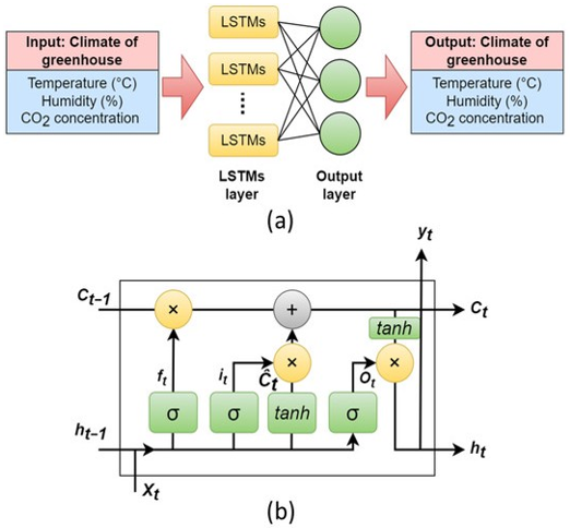
RNNs and their gated variants, LSTMs, excel at capturing temporal dependencies in sequential data, enabling accurate forecasting of greenhouse temperature, humidity, and CO2 concentration. These architectures are particularly well- suited for environmental monitoring due to their ability to maintain a hidden state that evolves through time, effectively modeling both short-term and long-term dependencies in sequential data.
6.2.1 LSTM cell architecture
The core strength of LSTM networks lies in their sophisticated gating mechanism, which prevents vanishing and exploding gradient problems that are commonly encountered in traditional RNNs. Figure 11 details the LSTM model architecture and, at the cell level, its three gates (input, forget, output) and the cell state that carries information across timesteps [84, 85]:
$f_t=\sigma\left(W_f\left[\begin{array}{c}h_{t-1} \\ x_t\end{array}\right]+b_f\right)$ (15)
$i_t=\sigma\left(W_i\left[\begin{array}{c}h_{t-1} \\ x_t\end{array}\right]+b_i\right)$ (16)
$\tilde{c}_t=\tanh \left(W_c\left[\begin{array}{c}h_{t-1} \\ x_t\end{array}\right]+b_c\right)$ (17)
$c_t=f_t \odot c_{t-1}+i_t \odot \tilde{c}_t$ (18)
$o_t=\sigma\left(W_0\left[\begin{array}{c}h_{t-1} \\ x_t\end{array}\right]+b_0\right)$ (19)
$h_t=i_t \odot \tanh \left(c_t\right)$ (20)
Figure 11. (a) Architecture of the long short-term memory (LSTM) model used in this study and (b) the structure of a single cell of LSTM
6.2.2 Environmental applications performance
Comparative studies show LSTM models often outperform traditional autoregressive models by maintaining long-term context, thereby reducing prediction errors such as RMSE and MAE in environmental monitoring applications [86]. Liu et al. [85] demonstrated that LSTMs reduced RMSE by up to 25% and MAE by 18% compared to ARIMA and SARIMA models when forecasting greenhouse CO2 and humidity. For multi-step forecasting up to 24 hours ahead, Jeon et al. [87] showed LSTMs maintained MAE <1.0 ℃ even at extended time horizons, while feedforward networks exhibited MAE > 1.5 ℃.
In typical greenhouse applications, stacked LSTM architectures with 2–3 layers (each containing 64 units) and dropout regularization (rate = 0.2) have proven effective, achieving test errors of approximately RMSE ≈ 0.8 ℃ and MAE ≈ 0.6 ℃ when trained using RMSprop optimization [88].
6.3 Transfer learning and fine-tuning strategies
Figure 12 outlines transfer learning has been the process by which a pre-trained model on large datasets (for example, ImageNet) is altered for customized usage, greatly saving the time needed for training as well as the data requirements [88]. Common fine-tuning approaches include retraining only the classifier layers, unfreezing the convolutional blocks gradually, or using adaptive learning rate schedules to avoid catastrophic forgetting [89, 90] Recently, a comparative study involving eight different kinds of fine-tuning has shown that, typically, full unfreezing of the layers followed by differential learning rates provide the marginal best accuracy to computational cost trade-off.
Figure 12. Transfer learning workflow
6.3.1 Pre-training and feature extraction
Models such as VGG16, ResNet50, and MobileNet, pre- trained on the ImageNet dataset (comprising 1.2 million images tagged into 1,000 classes), constitute powerful baseline starting points for transfer learning. These models have essentially learned to represent low-level features, such as edges and textures, that are broadly transmittable across domains. The pre- trained features are used effectively in agricultural applications to accomplish downstream classification tasks with as few as 500 labeled samples.
6.3.2 Best practices for agricultural applications
For agricultural datasets that often differ substantially from general image collections such as ImageNet, Zhao et al. [91]. propose self-supervised pre-training on unlabelled plant imagery as a way of bridging the domain gap before fine-tuning, pairing contrastive pre-training on large volumes of unlabelled leaf images with a domain adaptation layer that corrects for distribution shift during fine-tuning. In a broader review of transfer learning in agriculture, Hossen et al. [92]. likewise report that pre-trained backbones combined with standard augmentation strategies (such as rotation, colour jitter, and random erasing) are widely used to improve classification performance on small and imbalanced agricultural image datasets, where labelled samples are scarce.
The evidence surveyed here does not support a blanket preference for deep learning. On temporal forecasting and image-based diagnosis, deep models (LSTM, CNN) consistently reduce error relative to Support Vector Regression (SVR) and Random Forest (RF); in the head-to-head comparison, for example, the LSTM cut tomato-yield RMSE by roughly 60% over RF, because such models learn temporal and spatial structure directly rather than relying on hand-crafted features. That advantage, however, is contingent on data volume. On the small, low-dimensional tabular datasets typical of a single greenhouse season, classical models often match deep networks while being cheaper to train, easier to interpret, and far less prone to the over-fitting documented in Section 5.3. The practical implication is therefore a decision rule rather than a single winner: deep learning is preferable where sequential or visual data are abundant and edge compute permits, whereas classical machine learning remains the stronger choice where data are scarce, interpretability matters, or the deployment target is a low-power microcontroller. Table 8 consolidates the validated results of the surveyed studies, exposing their recurring strengths, shared limitations, and open gaps.
Table 8. Researches validated results comparison table
|
Study |
Category |
Method / Data |
Key Result |
Strengths |
Limitations / Gap |
|
ML vs. DL [87] |
ML vs. DL |
SVR, RF vs LSTM; UK tomato + Belgian Ficus, climate features |
LSTM RMSE 0.047 / 0.042 < SVR, RF |
Direct ML-DL contrast; temporal dynamics |
2 datasets only; yield interpolated; no external validation |
|
Liu et al. [85] |
DL / forecasting |
LSTM; greenhouse CO₂ and humidity series |
RMSE −25%, MAE −18% vs. ARIMA/SARIMA |
Retains long-term context |
Baselines only linear; site/scale |
|
Ferentinos [10] |
DL / CV |
CNN; large leaf-disease image set |
~99% classification |
Large-scale disease ID |
Lab images; field accuracy drops |
|
Kamilaris and Prenafeta-Boldu [23] |
Survey |
Meta-review of DL in agriculture |
DL > classical CV |
Broad synthesis |
No new experiments; pre-2018 |
|
El-Gayar et al. [11] |
IoT / edge |
Edge-cloud monitoring architecture |
|
Lower latency vs cloud-only |
Metrics / crop scope [verify] |
|
NDVI / multispectral [41] |
Sensing |
GreenSeeker / UAV NDVI; canopy vigor |
Index-based vigor mapping |
Canopy-scale, non-contact |
Illumination-sensitive; needs calibration |
Along the sensing modality axis, we contrast RGB, multispectral, and thermal imaging by what each measure, what it cannot, and its cost/robustness trade-offs.
7.1 Multispectral analysis
Multispectral imaging has emerged as a cornerstone in modern smart greenhouse systems, providing insights into plants physiology beyond what traditional RGB cameras can capture. While RGB imaging is akin to reading only the cover of a book, multispectral imaging lets researchers explore multiple internal chapters-each spectral band revealing a different physiological characteristic of the plant.
7.1.1 RGB Imaging vs multispectral imaging
RGB imaging utilizes three broad visible spectral bands: red (approximately 620–700 nm), green (495–570 nm), and blue (450–495 nm). It effectively captures color, structure and visible stress indicators such as chlorosis or wilting, all at relatively low cost and high spatial resolution. Multispectral imaging, by contrast, includes discrete non-visible bands such as Near-Infrared (NIR), Red Edge, or Short-Wave Infrared (SWIR), which reveal subtle spectral signatures linked to chlorophyll absorption, water content, and leaf cell structure. These additional bands enable computation of various vegetation indices that can detect crop stress nutrient deficiency, or disease before visible symptoms appear.
7.1.2 Key vegetation indices and metrics
Table 9 gathers the key vegetation indices computed from multispectral data:
•NDVI (Normalized Difference Vegetation Index): used worldwide as a proxy for greenness, biomass, and plant vigor.
•SAVI (Soil Adjusted Vegetation Index): Adjusts NDVI to reduce the effect of soil brightness.
•Red Edge Indices: Sensitive to changes due to early stress and variation in chlorophyll.
Table 9. Key vegetation indices
|
Index |
Formula |
Application |
|
NDVI |
$N D V I=\frac{N I R-\text { Red }}{N I R+\text { Red }}$ |
Vegetation vigor |
|
SAVI |
$N D V I=\frac{(N I R-\operatorname{Red})(1+L)}{N I R+R e d+L}$ |
Soil correction |
|
EVI |
$2.5 * \frac{N I R-\text { Red }}{N I R+6 \text { Red }-7.5 \text { Blue }+1}$ |
High biomass areas |
|
VARI |
$N D V I=\frac{\text { Green-Red }}{\text { Green+Red-Blue }}$ |
RGB-based vegetation |
|
RENDVI |
$N D V I=\frac{N I R-\text { RedEdge }}{N I R+\text { RedEdge }}$ |
Early stress detection |
Other RGB-based indices, like Red Edge Normalized Difference Vegetation Index (RENDVI) and Visible Atmospherically Resistant Index (VARI), are used for estimating vegetation health, but their performance is commonly limited under low contrast or early-stress conditions.
7.1.3 Areas of application in smart greenhouses
Multispectral imaging is considered better than alternatives for applications like plant health monitoring where it detects early nutrient deficiency and disease from red-edge and near infrared bands, water stress assessment NIR and red-edge reflectance strongly correlate with leaf water content for precision irrigation and canopy and biomass estimation where it facilitates canopy cover and leaf area index (LAI) measurements under variable illumination conditions more accurately.
For example, Burchard-Levine et al. [93] presented a multispectral 3D point-cloud approach which could measure the chlorophyll content for greenhouse tomatoes more accurately than 2D RGB methods; these estimations strongly correlated with SPAD meter readings. Likewise, Poirier-Pocovi et al. [94] also compared UAV-based RGB and multispectral indices for palm cultivation and reported that the multispectral system was more reliable under changing illumination.
7.1.4 Advantages and limitations of multispectral imaging
Multispectral imaging offers several advantages for smart greenhouse monitoring: by capturing reflectance in non-visible bands such as near infrared and red edge, it detects nutrient deficiency, water stress, and disease before symptoms become visible to RGB sensors, and it enables quantitative vegetation indices (NDVI, SAVI, red-edge) that correlate with chlorophyll content, biomass, and leaf water status. It is also non-destructive and scales from handheld to UAV and fixed-mount deployment. Its limitations, however, constrain low-cost adoption: multispectral cameras are markedly more expensive than RGB, their readings are sensitive to illumination and require radiometric calibration and, in field use, atmospheric correction, and the vegetation indices can saturate at high biomass or lose sensitivity under early or low-contrast stress. As with thermal imaging, the most robust results reported in the literature come from fusing multispectral data with RGB or thermal modalities rather than relying on any single sensor.
7.1.5 Integration and emerging trends
Emerging techniques focus on the fusion of RGB, multispectral, and thermal imaging for better accuracy. Integrating them into UAVs, fixed sensor networks, and roof-mounted greenhouse systems is becoming common. Machine Learning models such as Random Forests, Support Vector Regression, and Deep Neural Networks are increasingly employed to estimate chlorophyll content, biomass, and stress indicators using multispectral data.
7.2 Thermal imaging
Whereas multispectral imaging works with reflected radiation, thermal imaging works with infrared radiation, which is being emitted by plant surfaces and carries information on physiological processes that cannot be recorded by optical sensors.
Thermal imageries are emerging as a backbone to smart greenhouse systems to observe the physiological behavior of plants non-invasively contrary to RGB or multi-spectral imagers, which use reflected visible or near-infrared light, the thermal imagers record the emitted infrared radiation from plant surfaces in the wavelength of 8–14 µm. Thermal maps are considered a direct abstraction of insights regarding the transpiration rate, stomatal conductance, and water stress situations of crops [95].
In a conventional setting, the thermal camera views radio- metric temperature of leaves, which is in large measure directly correlated to water status in the plant. Plants undergo water deficit where the stomata close and transpiration gets reduced, in which case the leaf becomes warmer. This phenomenon forms the core behind indices like Crop Water Stress Index (CWSI), which is calculated from canopy temperature relative to reference temperature [96].
$C W S I=\frac{T_c-T_{w e t}}{T_{d r y}-T_{w e t}}$ (21)
where, $T_c$ is the canopy temperature, and $T_{\text {wet}}$ and $T_{d r y}$ are the reference temperatures for fully transpiring and non-transpiring leaves, respectively.
Thermal imaging can be applied for early stress detection, irrigation scheduling, and automated climate control in green- houses. For example, the study [97] has shown that coupling thermal sensors with IoT-based systems allows for the forming of real-time feedback loops to optimize irrigation and ventilation. Similarly, the combination of thermal and multispectral data improves the accuracy of stress detection and plant growth modeling [98]. Table 10 compares the RGB, multispectral, and thermal sensing modalities.
Cooling down the effects caused by field variations and camera calibration problems along with the background radiation often create matters for thermal imaging [99]. Future trends involve integrating thermal data with AI-based analytics and sensor fusion techniques for enhancing the smart greenhouse management decision-making.
Table 10. Modality comparison table
|
Modality |
What It Measures |
Main Strength |
Key Limitation |
|
Red, Green, Blue (RGB) |
Visible colour, structure, morphology |
Low cost, high resolution, simple |
Blind to pre-visual stress |
|
Multispectral |
Reflectance in NIR / red-edge / SWIR (vegetation indices) |
Detects nutrient/water stress before visible symptoms |
Needs calibration; illumination-sensitive; indices saturate |
|
Thermal |
Emitted infrared (canopy temperature) |
Detects water stress early; lighting-independent |
Ambient/emissivity sensitive; cannot identify the cause |
7.2.1 Advantages and limitations of thermal imaging
Thermal imaging offers several advantages for smart greenhouse management: it enables non-invasive monitoring of plant physiological status by measuring emitted infrared radiation, providing real-time feedback on transpiration rate, stomatal conductance, and water stress, and, unlike optical imaging, it operates independently of ambient lighting to maintain consistent measurements from day to night; furthermore, thermal data can be integrated with IoT and AI-based systems for automated irrigation scheduling, early stress detection, and precise climate control, and when combined with multispectral imaging it supports far more accurate crop stress diagnosis and growth modeling. However, the technology also has notable limitations: it is highly sensitive to environmental variations such as wind, humidity, and background radiation that distort temperature readings. It depends on critical yet complicated camera calibration and emissivity correction to ensure accuracy; the high cost of thermal sensors and the intricate data-processing algorithms they require limit large-scale adoption in low-cost commercial greenhouses; and thermal imaging alone typically cannot distinguish between sources of temperature variation. For example, whether a change stems from disease or water deficit requires the combination with other sensing technologies for robust decision-making.
Although smart greenhouses technologies show immense potential to increase productivity, efficiency, and sustainability, their adoption on a larger scale confronts integration problems. This section discusses points on barriers and opportunities concerning interoperability, cost and scalability, and data security.
8.1 Interoperability issues
Different types of sensors, communication protocols, and control systems often create fragmented architectures, which do not support a smooth integration process. Many commercial and many other open-source platforms are interoperable only to a limited extent, requiring the use of middleware or mechanism translations in the protocols to run their devices in unison [99, 100] Standardization bodies such as the Open Geospatial Consortium (OGC) Sensor Things API and ISO 11783 (ISOBUS) attempt to solve this problem; however, it is not uniformly adopted in different regions and by all manufacturers. There is an opportunity to provide modular, vendor- neutral architectures that allow plug-and-play device integration, thus greatly reducing deployment time and maintenance complexity.
8.2 Cost and scalability
One of the entry barriers for small- and medium-sized farms, especially in developing regions, is high upfront capital expenditures. Costs cover sensors and actuators, IoT infrastructure, cloud services, and ongoing servicing [101]. Low-cost microcontrollers (such as ESP32) and free and open-source platforms (e.g., Node-RED, Things Board) offer scalable implementations to lower entry barriers. Additionally, edge computing architectures reduce recurring cloud service charges by processing data locally [102]. From a scalability perspective, a modular system design can be preferable, in that it allows system expansion following availability of resources, rather than full-scale deployment all at once.
8.3 Data security and privacy
The integrated IoT and cloud platform introduces vulnerabilities in terms of data confidentiality, integrity, and availability [103]. The threats include unauthorized access, interception, and hijacking of devices through insecure protocols. Best practices include:
•Implementing secure communication protocols (TLS over MQTT, HTTPS)
•Regular firmware updates and patch management
•Network segmentation to isolate critical control devices from public-facing networks
Privacy concerns also arise when operational and environmental data in high resolution is collected, as it could be used to infer proprietary crop management practices if leaked. Policy frameworks and data governance models tailored to agriculture can help address these concerns while enabling collaborative research and benchmarking.
8.4 Comparative study of machine learning and deep learning for greenhouse prediction
Alhnaity et al. [100] compared the predictive ability of conventional machine learning methods versus that of deep learning models within prototypical greenhouse environments. Table 11 present that comparison. SVR and RF were considered as classical baseline machine learning models, while an LSTM network was implemented as deep learning.
There were two greenhouse datasets. The first, collected in Belgium, included Ficus Benjamina growth data (stem diameter) and microclimatic variables such as temperature, relative humidity, CO2 concentration, and photosynthetically active radiation. The second one, coming from a UK commercial greenhouse, contained environmental factors with tomato yields. Interpolation was done from weekly yield data to daily values to merge temporal resolutions. All datasets were divided into training (60%), validation (15%), and testing (25%) fractions. MSE, RMSE, and MAE were used to assess model performance.
Table 11. Performance of ML (SVR, RF) and DL (LSTM) models for greenhouse plant yield and growth prediction [98]
|
|
Tomato Yield |
Ficus Growth (SDV) |
||||
|
Metric |
SVR |
RF |
LSTM |
SVR |
RF |
LSTM |
|
MSE |
0.015 |
0.040 |
0.002 |
0.006 |
0.006 |
0.001 |
|
RMSE |
0.125 |
0.200 |
0.047 |
0.073 |
0.062 |
0.042 |
|
MAE |
0.087 |
0.192 |
0.030 |
0.070 |
0.063 |
0.030 |
As shown in Table 11, the LSTM model consistently achieved lower error values than the traditional SVR and RF models across both datasets. For tomato yield prediction, LSTM reduced the RMSE to 0.047, compared to 0.125 (SVR) and 0.200 (RF). Similarly, for Ficus Benjamina stem diameter variation (SDV), LSTM achieved the lowest RMSE (0.042) and MSE (0.001). Figures provided by the authors; further illustrate that the LSTM model not only tracked the temporal trends of plant growth and yield more closely but also generalized better to unseen data, highlighting its superior ability to capture time- dependent patterns in greenhouse environments. The results showed a consistent superiority of the LSTM network over traditional machine learning methods in both experiments. While SVR and RF did provide reasonable predictions for yield, they were less ac- curate and were unable to reproduce good temporal dynamics for plant growth and yield. LSTMs can learn long-term dependencies from time series data, thus dramatically reducing prediction errors and justifying their use in greenhouse production- wise forecasts.
These results should not be read as a general verdict that deep learning is always superior. The LSTM outperformed SVR and RF here specifically because greenhouse yield and growth are governed by time-dependent processes that a recurrent model can learn directly from sequential data, whereas the classical models discard that temporal structure. The same advantage would be expected to narrow, or even reverse, on small tabular datasets, on tasks without a temporal dimension, or where model interpretability and low power inference are decisive. The practical takeaway is thus conditional: LSTM-based models are the stronger choice for sequential greenhouse forecasting given sufficient data, while classical machine learning remains competitive and often more practical for smaller-scale or resource-constrained deployments.
In this coming decade, smart greenhouse systems will experience tremendous changes due to the rapid development of sensing technologies, IoT architectures, and artificial intelligence. Chief among the proposed developmental trajectories is the enhanced path towards AI-driven agricultural intelligence and the interference of edge technology with digital twin frameworks.
9.1 Trends in AI driven agriculture
Agricultural AI systems are expected to transition from single-task applications such as disease detection or yield estimation toward multi-task learning architectures capable of simultaneously managing multiple greenhouse control processes. These models will integrate heterogeneous data streams, including visual, climatic, and soil measurements, to coordinate irrigation, climate regulation, and pest management in a unified framework.
Recent advances in few-shot learning and federated learning are likely to address two major limitations of current agricultural AI systems: the scarcity of labeled datasets and concerns related to data privacy among stakeholders. Federated learning, in particular, enables collaborative model training across multiple greenhouse sites without requiring the exchange of raw data. In parallel, the integration of AI with autonomous robotic platforms such as mobile units for precision spraying, automated harvesting, and plant inspection is gaining increasing attention. These continuously operating systems not only enhance operational efficiency but also generate additional data streams that further enrich AI-driven decision-making.
9.2 Edge-computing and digital-twins perspective
Cloud-centric greenhouse control architectures are often constrained by latency, bandwidth requirements, and intermittent connectivity, especially in rural or remote agricultural environments. Edge computing addresses these limitations by enabling local processing of sensor data on embedded devices, thereby supporting real-time control even in the absence of continuous internet connectivity. Edge AI accelerators, such as NVIDIA Jetson and Google Coral platforms, allow inference tasks such as image-based disease recognition or short-term climate prediction to be executed directly within the greenhouse environment.
In parallel, digital twin technology introduces a virtual representation of the physical greenhouse that remains synchronized with real-time sensor data. This virtual counterpart enables the simulation and evaluation of control strategies before physical deployment, reducing the risk of crop stress and operational failures. Digital twins further support yield optimization, resource and energy efficiency analysis, and “what-if” scenario evaluation under climate anomalies [103].
The combination of edge computing and digital twins facilitates hybrid architectures in which high-frequency sensor data and real-time simulations are processed locally, while cloud platforms are leveraged periodically for long-term analytics, data storage, and collaborative model improvement. Collectively, these developments point toward the emergence of self-optimizing greenhouse systems that operate with minimal human intervention while maximizing productivity and resource efficiency.
The smart greenhouses have evolved from simple transparent structures that were manually maintained into highly sophisticated cyber-physical environments equipped with sensing, communication, actuation, and artificial intelligence. This was the result of the rapid growth in sensor technology, IoT protocols, and machine-learning algorithms that provide continuous monitoring, predictive analytics, and autonomous crop and climate management.
Research and techno-development have, in due course, demonstrated the feasibility of yield prediction, irrigation, fertilization, and disease control management through a range of such systems. But there are several issues that still need to be resolved. Large-scale deployment, especially in the less-developed world, is still curtailed due to the issues in interoperability, very high costs of implementation, and data- insecure infrastructures. Hence, frameworks for standards, cheap modular architectures, and data exchange mechanisms of preserving privacy are called for. Tackling these will be needed for the wider uptake of smart greenhouse technology.
Given the trends in the current era, it is expected that artificial intelligence, autonomous robotics, edge computing, and digital twin modeling will converge to create self- optimizing greenhouse systems, which can adapt to environmental changes autonomously Such technologies are great instruments to enhance food security, optimize resource use efficiency, and make global agriculture sustainable.
Despite substantial progress in smart greenhouse technologies, several research challenges remain open and require systematic investigation. Unlike the broader technological outlook discussed in Section 9, this section identifies specific research directions that are critical for advancing the state of the art.
AI-driven predictive control remains a key research priority, requiring the development of adaptive models capable of learning from multisource sensor data and responding to dynamic greenhouse conditions. Sensor fusion and hardware miniaturization represent another important direction, aiming to combine thermal, multispectral, and hyperspectral sensing within cost-effective IoT frameworks to achieve high-resolution plant monitoring.
Energy-efficient system design also warrants further exploration, particularly through the integration of renewable energy sources, intelligent energy management strategies, and smart materials to reduce operational costs and environmental impact. In parallel, effective coordination between edge and cloud computing resources remains an open challenge, necessitating optimized task allocation strategies that balance latency, scalability, and computational efficiency.
Finally, standardization and interoperability issues must be addressed to enable seamless communication among heterogeneous devices and platforms. Socio-economic and ethical considerations, including affordability, accessibility, data governance, and sustainability, are equally important to ensure large-scale adoption across diverse agricultural contexts.
The authors gratefully acknowledge the full financial support provided by BI Engineering Tech. Their contribution was essential in enabling the completion of this review.
|
$y_i$ |
Actual value (true label, ground truth). |
|
$\widehat{y_l}$ |
Predicted value by the model. |
|
$\bar{y}$ |
Mean of the actual values. |
|
n |
Total number of data points. |
|
TP |
True Positives (correctly predicted positive cases). |
|
TN |
True Negatives (correctly predicted negative cases). |
|
FP |
False Positives (incorrectly predicted as positive) |
|
FN |
False Negatives (missed positive cases). |
[1] Maraveas, C. (2023). Incorporating artificial intelligence technology in smart greenhouses: Current state of the art. Applied Sciences, 13(1): 14. https://doi.org/10.3390/app13010014
[2] Zabeltitz, C. (2011). Integrated greenhouse systems for mild climates: Climate conditions, design, construction, maintenance, climate control. Springer. https://doi.org/10.1007/978-3-642-14582-7
[3] Castilla, N. (2013). Greenhouse technology and management (2nd ed.). CABI. https://rexresearch1.com/GreenhouseLibrary/GreenhouseTechnologyManagement.pdf.
[4] Shamshiri, R., Kalantari, F., Ting, K.C., et al. (2018). Advances in greenhouse automation and controlled environment agriculture: A transition to plant factories and urban agriculture. International Journal of Agricultural and Biological Engineering, 11(1): 1-22. https://doi.org/10.25165/j.ijabe.20181101.3210
[5] Ameer, S., Ibrahim, H., Kulsoom, F., Ameer, G., Sher, M. (2024). Real-time detection and measurements of nitrogen, phosphorous potassium from soil samples: A comprehensive review. Journal of Soils and Sediments, 24: 1-19. https://doi.org/10.1007/s11368-024-03827-5
[6] Kalaany, C.M.A., Kimaita, H.N., Abdelmoneim, A.A., Khadra, R., Derardja, B., Dragonetti, G. (2025). The potential of low-cost IoT-enabled agrometeorological stations: A systematic review. Sensors, 25(19): 6020. https://doi.org/10.3390/s25196020
[7] Prasad, S.R.S.S., Rao, P.V.R.D.P., Mohan, K.R.R. (2022). Implementation of a LoRaWAN based smart agriculture decision support system for optimum crop yield. Sustainability, 14(2): 827. https://doi.org/10.3390/su14020827
[8] Tripathi, P., Kumar, N., Rai, M., Shukla, P.K., Verma, K.N. (2023). Applications of machine learning in agriculture. In Smart Village Infrastructure and Sustainable Rural Communities, IGI Global Scientific Publishing, pp. 99-118. https://doi.org/10.4018/978-1-6684-6418-2.ch006
[9] El Ouaham, W., Sadik, M., Ennajih, A., Mouzouna, Y., Orchi, H., Elouaham, S. (2026). Smart greenhouses in the era of IoT and AI: A comprehensive review of AI applications, spectral sensing, multimodal data fusion, and intelligent systems. Agriculture, 16(7): 761. https://doi.org/10.3390/agriculture16070761
[10] Ferentinos, K.P. (2018). Deep learning models for plant disease detection and diagnosis. Computers and Electronics in Agriculture, 145: 311-318. https://doi.org/10.1016/j.compag.2018.01.009
[11] El-Gayar, A., Soliman, M., Hassanien, A.E. (2025). Edge-cloud monitoring system for smart vertical farming. CEUR Workshop Proceedings, 4110: 88-99. https://ceur-ws.org/Vol-4110/paper10.pdf.
[12] Wang, L., He, X.F., Luo, D.J. (2020). Deep reinforcement learning for greenhouse climate control. In 2020 International Conference on Big Knowledge, Nanjing, China, pp. 474-480. https://doi.org/10.1109/ICBK50248.2020.00073
[13] Montero, J.I., Muñoz, P., Baeza, E., Stanghellini, C. (2017). Ongoing developments in greenhouse climate control. Acta Horticulturae, 1182: 1-14. https://doi.org/10.17660/ActaHortic.2017.1182.1
[14] Papadakis, G., Briassoulis, D., Scarascia-Mugnozza, G., Vox, G., Feuilloley, P., Stoffers, J.A. (2000). Radiometric and thermal properties of, and testing methods for, greenhouse covering materials. Journal of Agricultural Engineering Research, 77(1): 7-38. https://doi.org/10.1016/S0021-8634(00)0007-X
[15] Abdel-Ghany, A.M., Al-Helal, I.M. (2011). Solar energy utilization by a greenhouse: General relations. Renewable Energy, 36(1): 189-196. https://doi.org/10.1016/j.renene.2010.06.020
[16] Sharma, A., Tyagi, V.V., Chen, C.R., Buddhi, D. (2009). Review on thermal energy storage with phase change materials and applications. Renewable and Sustainable Energy Reviews, 13(2): 318-345. https://doi.org/10.1016/j.rser.2007.10.005
[17] Nishad, S., Krupa, I. (2022). Phase change materials for thermal energy storage applications in greenhouses: A review. Sustainable Energy Technologies and Assessments, 52: 102241. https://doi.org/10.1016/j.seta.2022.102241
[18] Et-taibi, B., Abid, M.R., Boumhidi, I. (2020). Smart agriculture as a cyber physical system: A real-world deployment. In 2020 International Conference on Digital Society, Fez, Morocco, pp. 1-7. https://doi.org/10.1109/ICDS50568.2020.9268734
[19] Gueye, P.E.A., Deme, C.B., Ngom, D., Basse, A. (2025). Hybrid improved stacking over tabular temporal features with blockchain-certified data: Millet yield prediction and explainability. Information Dynamics and Applications, 4(4): 238-256. https://doi.org/10.56578/ida040405
[20] Yu, J.X., Sun, C.C., Zhao, J.P., et al. (2025). Prediction and control of greenhouse temperature: Methods, applications, and future directions. Computers and Electronics in Agriculture, 237: 110603. https://doi.org/10.1016/j.compag.2025.110603
[21] Hu, G.Q., Kubota, C., You, F.Q. (2025). Cyber physical biological system in controlled environment agriculture for energy optimization: A comprehensive overview, key challenges, and future outlook. Energy, 325: 136153. https://doi.org/10.1016/j.energy.2025.136153
[22] Avşar, E., Mowla, M.N. (2022). Wireless communication protocols in smart agriculture: A review on applications, challenges and future trends. Ad Hoc Networks, 136: 102982. https://doi.org/10.1016/j.adhoc.2022.102982
[23] Kamilaris, A., Prenafeta-Boldu, F.X. (2018). Deep learning in agriculture: A survey. Computers and Electronics in Agriculture, 147: 70-90. https://doi.org/10.1016/j.compag.2018.03.012
[24] Bersani, C., Ruggiero, C., Sacile, R., Soussi, A., Zero, E. (2022). Internet of things approaches for monitoring and control of smart greenhouses in industry 4.0. Energies, 15(10): 3834. https://doi.org/10.3390/en15103834
[25] Praveena, M., Babiyola, A., Aghalya, S., Sasikar, A. (2023). Wireless sensor network based greenhouse monitoring using cloud integration with data analytics. In 2023 2nd International Conference on Edge Computing and Applications, Namakkal, India, pp. 68-72. https://doi.org/10.1109/ICECAA58104.2023.10212251
[26] Drouaillet-Mejía, Z., Fernández-Echeverría, E., Silva-Martínez, W.A., Ortega-Gijón, Y.N., Fernández-Lambert, G., García-Santamaría, L.E. (2025). Water efficiency in polycultures for small-scale agriculture. Revista Mexicana De Ciencias Agrícolas, 16(6): e3821. https://doi.org/10.29312/remexca.v16i6.3821
[27] Saban, M., Bekkour, M., Amdaouch, I., et al. (2023). A smart agricultural system based on PLC and a cloud computing web application using LoRa and LoRaWan. Sensors, 23(5): 2725. https://doi.org/10.3390/s23052725
[28] Yousef, K. (2021). Environmental monitoring in greenhouse agriculture using IoT and wireless sensor networks. Sensors, 21(12): 4074. https://doi.org/10.3390/s21124074
[29] Kim, H.J., Lee, M.H. (2026). A comparative performance study of parallel MQTT and RS485 communication architectures for high-frequency IoT sensing. Electronics, 15(4): 760. https://doi.org/10.3390/electronics15040760
[30] Ojha, T., Misra, S., Raghuwanshi, N.S. (2015). Wireless sensor networks for agriculture: The state-of-the-art in practice and future challenges. Computers and Electronics in Agriculture, 118: 66-88. https://doi.org/10.1016/j.compag.2015.08.011
[31] Lazarescu, M.T. (2013). Design of a WSN platform for long-term environmental monitoring for IoT applications. IEEE Journal on Emerging and Selected Topics in Circuits and Systems, 3(1): 45-54. https://doi.org/10.1109/JETCAS.2013.2243032
[32] Pooja, S., Uday, D.V., Nagesh, U.B., Talekar, S.G. (2017). Application of MQTT protocol for real time weather monitoring and precision farming. In 2017 International Conference on Electrical, Electronics, Communication, Computer, and Optimization Techniques, Mysuru, India, pp. 1-6. https://doi.org/10.1109/ICEECCOT.2017.8284616
[33] Hunkeler, U., Truong, H.L., Stanford-Clark, A. (2008). MQTT-s—A publish/subscribe protocol for wireless sensor networks. In 2008 3rd International Conference on Communication Systems Software and Middleware and Workshops, Bangalore, India, pp. 791-798. https://doi.org/10.1109/COMSWA.2008.4554519
[34] Abdelmadjid, M.K., Noureddine, S., Amina, B., Khelifa, B., Tariq, B., Boubakeur, L. (2022). IoT and WSNs technology for control in the greenhouse agriculture - Review. In 2022 3rd International Conference on Embedded & Distributed Systems, Oran, Algeria, pp. 136-141. https://doi.org/10.1109/EDiS57230.2022.9996500
[35] T, G.K., Shashank, K.V. (2022). Smart farming based on AI, edge computing and IoT. In 2022 4th International Conference on Inventive Research in Computing Applications, Coimbatore, India, pp. 324-327. https://doi.org/10.1109/ICIRCA54612.2022.9985023
[36] Al-Fuqaha, A., Guizani, M., Mohammadi, M., Aledhari, M., Ayyash, M. (2015). Internet of things: A survey on enabling technologies, protocols, and applications. IEEE Communications Surveys & Tutorials, 17(4): 2347-2376. https://doi.org/10.1109/COMST.2015.2444095
[37] AutoMQ Team. (2025). MQTT vs. Apache Kafka: A Deep Dive into Messaging Technologies. https://www.automq.com/blog/mqtt-vs-apache-kafka-messaging-technologies.
[38] Adelantado, F., Vilajosana, X., Tuset-Peiro, P., Martínez, B., Melia-Seguí, J., Watteyne, T. (2017). Understanding the limits of LoRaWAN. IEEE Communications Magazine, 55(9): 34-40. https://doi.org/10.1109/MCOM.2017.1700668
[39] Eureka Patsnap. (2025). LoRa’s chirp spread spectrum: Enabling long-range IoT connectivity. https://eureka.patsnap.com/article/loras-chirp-spread-spectrum-enabling-long-range-iot-connectivity.
[40] Glaroudis, D., Iossifides-Iosifidis, A., Chatzimisios, P. (2019). Survey, comparison and research challenges of IoT application protocols for smart farming. Computer Networks, 165: 107037. https://doi.org/10.1016/j.comnet.2019.107037
[41] Sifawa, H.A., Tambawal, A.B., Tudu, S.M. (2026). Performance evaluation of IoT protocols in resource-constraints smart home networks. International Journal of Science and Global Sustainability, 12(1): 48-61. https://doi.org/10.57233/ijsgs.v12i1.1012
[42] Naik, N. (2017). Choice of effective messaging protocols for IoT systems: MQTT, CoAP, AMQP and HTTP. In 2017 IEEE International Systems Engineering Symposium, Vienna, Austria, pp. 1-7. https://doi.org/10.1109/SysEng.2017.8088251
[43] Marini, R., Cuozzo, G. (2025). Next generation LoRaWAN: Integrating multi-hop communications at 2.4 GHz. arXiv preprint arXiv:2504.00489. https://doi.org/10.48550/arXiv.2504.00489
[44] Fujii, A. (2019). Agricultural application of web of things architecture. Impact, 2019(10): 61-63. https://doi.org/10.21820/23987073.2019.10.61
[45] Microchip Technology. (2026). Microchip expands edge AI and embedded control for smart farming automation. EverythingPE. https://www.everythingpe.com/News/details/10372-microchip-expands-edge-ai-and-embedded-control-for-smart-farming-automation.
[46] Amiroh, K., Priyambodo, T.K., Lelono, D. (2025). A modular intelligent resource architecture: Optimizing QoS in edge-cloud fusion systems for smart agriculture. Engineering, Technology & Applied Science Research, 15(5): 27696-27702. https://doi.org/10.48084/etasr.12909
[47] Madapathage Don, W.S., Ahmed, M.R., Siraj, M., Anjum, R., Sha, H.H., Raja Rani, T. (2023). Monitoring plant growth in plant factories: A smart IoT solution. In International Conference on Big Data, IoT and Machine Learning, pp. 977-989. https://doi.org/10.1007/978-981-99-8937-9_65
[48] System properties comparison InfluxDB vs. OpenTSDB vs. TimescaleDB. DBEngines. https://dbengines.com/en/system/InfluxDB%3BOpenTSDB%3BTimescaleDB.
[49] Sage, R.F., Kubien, D.S. (2007). The temperature response of C3 and C4 photosynthesis. Plant, Cell & Environment, 30(8): 1086-1106. https://doi.org/10.1111/j.1365-3040.2007.01682.x
[50] Myster, J., Moe, R. (1996). Effect of diurnal temperature alternations on plant morphology in some greenhouse crops—A mini review. Scientia Horticulturae, 62(4): 205-215. https://doi.org/10.1016/0304-4238(95)00783-P
[51] Koidra. (2025). Grower's guide to calculated metrics—Episode 1: Vapor pressure deficit (VPD). https://www.koidra.ai/news-horticulture/growers-guide-to-calculated-metrics-episode-1-vapor-pressure-deficit-vpd/.
[52] Mahmoud, M., BenRejeb, I., Punja, Z.K., Buirs, L., Jabaji, S. (2023). Understanding bud rot development, caused by Botrytis cinerea, on cannabis (Cannabis sativa L.) plants grown under greenhouse conditions. Botany, 101(7): 200-231. https://doi.org/10.1139/cjb-2022-0139
[53] Panáček, D., Kupka, V., Nalepa, M.A. (2026). Printing technologies for monitoring crop health. Nature Communications, 17: 2009. https://doi.org/10.1038/s41467-026-68778-6
[54] Azizi, S., Aliniaeifard, S., Zarbakhsh, S., Esmaeili, S., Baghalian, K., Gruda, N.S. (2025). Photobiology, photosynthesis, and plant responses under artificial lighting in controlled environment agriculture. Scientia Horticulturae, 349: 114248. https://doi.org/10.1016/j.scienta.2025.114248
[55] El Hou, M., Zahidi, Y., Rabbah, N., El-Moufid, M., Medromi, H., Touati, A. (2025). Review of AI methods in precision agriculture. E3S Web of Conferences, 680: 00077. https://doi.org/10.1051/e3sconf/202568000077
[56] Pal, A.K., Patro, B.D.K., Chaube, S. (2026). Design and implementation of a deep learning framework for automated crop classification and health diagnosis in precision agriculture. Scientific Reports, 16: 11436. https://doi.org/10.1038/s41598-026-42151-5
[57] Chaudhary, P., Gulia, P., Gill, N.S. (2026). An evaluation of machine learning for soil analysis in internet of things-enabled smart farming. Scientific Reports, 16: 10318. https://doi.org/10.1038/s41598-026-36017-z
[58] Huang, Q.Y., Zhao, T.F. (2024). Data collection and labeling techniques for machine learning. arXiv preprint arXiv:2407.12793. https://doi.org/10.48550/arXiv.2407.12793
[59] Zhang, J.Y., Hsieh, C.Y., Yu, Y., Zhang, C., Ratner, A. (2022). A survey on programmatic weak supervision. arXiv Preprint arXiv:2202.05433. https://doi.org/10.48550/arXiv.2202.05433
[60] Ko, K.I., Kang, B., Yoe, H. (2026). Research on KS standard-based outlier classification and intelligent cleaning framework for smart greenhouse sensor data. Journal of The Korea Society of Computer and Information, 31(3): 199-208. https://doi.org/10.9708/jksci.2026.31.03.199
[61] Ripan, R.C., Sarker, I.H., Anwar, M.M., et al. (2021). An isolation forest learning based outlier detection approach for effectively classifying cyber anomalies. In Hybrid Intelligent Systems (HIS 2020), Advances in Intelligent Systems and Computing, pp. 270-279. https://doi.org/10.1007/978-3-030-73050-5_27
[62] Miller, C., Portlock, T., Nyaga, D.M., O’Sullivan, J.M. (2024). A review of model evaluation metrics for machine learning in genetics and genomics. Frontiers in Bioinformatics, 4: 1457619. https://doi.org/10.3389/fbinf.2024.1457619
[63] Rainio, O., Teuho, J., Klén, R. (2024). Evaluation metrics and statistical tests for machine learning. Scientific Reports, 14(1): 6086. https://doi.org/10.1038/s41598-024-56706-x
[64] Paleyes, A., Urma, R.G., Lawrence, N.D. (2023). Challenges in deploying machine learning: A survey of case studies. ACM Computing Surveys, 55(6): 114. https://doi.org/10.1145/3533378
[65] Peitz, S., Hotegni, S.S. (2024). Multi-objective deep learning: Taxonomy and survey of the state of the art. Machine Learning with Applications, 21: 100700. https://doi.org/10.1016/j.mlwa.2025.100700
[66] Heymann, H.H., Mende, H., Frye, M., Schmitt, R.H. (2023). Assessment framework for deployability of machine learning models in production. Procedia CIRP, 118: 32-37. https://doi.org/10.1016/j.procir.2023.06.007
[67] Caron, M., Misra, I., Mairal, J., Goyal, P., Bojanowski, P., Joulin, A. (2020). Unsupervised learning of visual features by contrasting cluster assignments. In NIPS'20: Proceedings of the 34th International Conference on Neural Information Processing Systems, Vancouver, Canada, pp. 9912-9924.
[68] Dihanster, W., Berton, L. (2023). A systematic review for class-imbalance in semi-supervised learning. Artificial Intelligence Review, 56(Suppl 2): 2349-2382. https://doi.org/10.1007/s10462-023-10579-0
[69] Sutton, R.S., Barto, A.G. (2018). Reinforcement learning: An introduction 2nd ed. MIT press Cambridge, 1(2): 25. https://mitpress.mit.edu/9780262039246/reinforcement-learning/.
[70] Reiter, R., Hoffmann, J., Reinhardt, D., et al. (2026). Synthesis of model predictive control and reinforcement learning: Survey and classification. Annual Reviews in Control, 61: 101045. https://doi.org/10.1016/j.arcontrol.2026.101045
[71] Schulman, J., Wolski, F., Dhariwal, P., Radford, A., Klimov, O. (2017). Proximal policy optimization algorithms. arXiv preprint arXiv:1707.06347. https://doi.org/10.48550/arXiv.1707.06347
[72] Kaiser, L., Babaeizadeh, M., Milos, P., et al. (2019). Model-based reinforcement learning for Atari. arXiv preprint arXiv:1903.00374. https://doi.org/10.48550/arXiv.1903.00374
[73] Wibisono, A., Song, H.K., Lee, B.M. (2025). A survey of multi-agent reinforcement learning for cooperative control in multi-AUV systems. IEEE Access, 13: 1-11. https://doi.org/10.1109/ACCESS.2025.3609457
[74] Padilla-Nates, J.P., Garcia, L.D., Lozoya, C., Orona, L., Cortes-Perez, A. (2025). Greenhouse irrigation control based on reinforcement learning. Agronomy, 15(12): 2781. https://doi.org/10.3390/agronomy15122781
[75] Charilaou, P., Battat, R. (2022). Machine learning models and over-fitting considerations. World Journal of Gastroenterology, 28(5): 605-607. https://doi.org/10.3748/wjg.v28.i5.605
[76] Subramanian, J., Simon, R. (2013). Overfitting in prediction models - Is it a problem only in high dimensions? Contemporary Clinical Trials, 36: 636-641. https://doi.org/10.1016/j.cct.2013.06.011
[77] Aliferis, C., Simon, G. (2024). Overfitting, underfitting and general model overconfidence and under-performance pitfalls and best practices in machine learning and AI. In G.J. Simon, C. Aliferis (Eds.), Artificial intelligence and machine learning in health care and medical sciences. https://doi.org/10.1007/978-3-031-39355-6_10
[78] Balestriero, H.R., Bottou, L., LeCun, Y. (2022). The effects of regularization and data augmentation are class dependent. arXiv Preprint arXiv:2204.03632. https://doi.org/10.48550/arXiv.2204.03632
[79] Ghasemzadeh, H., Hillman, R.E., Mehta, D.D. (2024). Toward generalizable machine learning models in speech, language, and hearing sciences: Estimating sample size and reducing overfitting. Journal of Speech, Language, and Hearing Research, 67(3): 753-781. https://doi.org/10.1044/2023_JSLHR-23-00273
[80] Habibi, L.N., Matsui, T., Tanaka, T.S.T. (2024). Critical evaluation of the effects of a cross-validation strategy and machine learning optimization on the prediction accuracy and transferability of a soybean yield prediction model using UAV-based remote sensing. Journal of Agriculture and Food Research, 16: 101096. https://doi.org/10.1016/j.jafr.2024.101096
[81] Guo, Z., Feng, L. (2024). Multi-step prediction of greenhouse temperature and humidity based on temporal position attention LSTM. Stochastic Environmental Research and Risk Assessment, 38: 4907-4934. https://doi.org/10.1007/s00477-024-02840-x
[82] Kislay, K., Singh, S., Joshi, S., et al. (2024). Evaluating K-fold cross validation for transformer based symbolic regression models. arXiv preprint arXiv.2410.21896. https://doi.org/10.48550/arXiv.2410.21896
[83] Sikati, J., Nouaze, J.C. (2023). YOLO-NPK: A lightweight deep network for lettuce nutrient deficiency classification based on improved YOLOv8 Nano. Engineering Proceedings, 58(1): 31. https://doi.org/10.3390/ecsa-10-16256
[84] Hochreiter, S., Schmidhuber, J. (1997). Long short-term memory. Neural Computation, 9(8): 1735-1780. https://doi.org/10.1162/neco.1997.9.8.1735
[85] Liu, W., Li, Y., Yang, M., et al. (2025). Microclimate prediction of solar greenhouse with pad-fan cooling systems using a machine and deep learning approach. Agriculture, 15(20): 2107. https://doi.org/10.3390/agriculture15202107
[86] He, J., Belien, T., Alhmedi, A., et al. (2025). Deep transfer learning for Codling moth damage detection in ‘Conference’ pear using X-ray radiography. Food Control, 183: 111923. https://doi.org/10.1016/j.foodcont.2025.111923
[87] Jeon, Y.J., Park, S.J., Lee, H., Cui, J.S., Jung, D.H. (2025). Emulating expert environmental control strategies in strawberry greenhouses using attention-LSTM. Information Processing in Agriculture. https://doi.org/10.1016/j.inpa.2025.12.002
[88] Azubuike, B.N., Chlingaryan, A., Correa-Luna, M., Clark, C.E., Garcia, S.C. (2026). Transfer learning and stacking ensembles for biomass estimation from smartphone imagery in pasture-based dairy systems. Journal of Agriculture and Food Research, 28: 102923. https://doi.org/10.1016/j.jafr.2026.102923
[89] Ranasinghe, N.G., Saeed, N., Sadeghian, P. (2026). Comparative analysis of LSTM and SARIMA for global temperature forecasting: Impact of regional trends and emissions. Climate, 14(3): 72. https://doi.org/10.3390/cli14030072
[90] Jones, H.G., Vaughan, R.A. (2004). Remote Sensing of Vegetation: Principles, Techniques, and Applications. Oxford University Press.
[91] Hossen, M.I., Awrangjeb, M., Pan, S., Al Mamu, A. (2025). Transfer learning in agriculture: A review. Artificial Intelligence Review 58: 97. https://doi.org/10.1007/s10462-024-11081-x
[92] Zhao, R.Z., Zhu, Y.C., Li, Y.H. (2023). CLA: A self-supervised contrastive learning method for leaf disease identification with domain adaptation. Computers and Electronics in Agriculture, 107967: 211. https://doi.org/10.1016/j.compag.2023.107967
[93] Burchard-Levine, V., Guerra, J.G., Borra-Serrano, I. (2024). Evaluating the utility of combining high resolution thermal, multispectral and 3D imagery from unmanned aerial vehicles to monitor water stress in vineyards. Precision Agriculture, 25: 2447-2476. https://doi.org/10.1007/s11119-024-10179-0
[94] Poirier-Pocovi, M., Volder, A., Bailey, B.N. (2020). Modeling of reference temperatures for calculating crop water stress indices from infrared thermography. Agricultural Water Management, 233: 106070. https://doi.org/10.1016/j.agwat.2020.106070
[95] Baluja, J., Diago, P., Balda, B., et al. (2012). Assessment of vineyard water status by thermal imagery: Optimization of data acquisition and analysis. Irrigation Science, 30(6): 431-442. https://doi.org/10.1007/s00271-012-0106-8
[96] Johnston, M., Andreu, A., Verfaillie, J., Baldocchi, D., González-Dugo, M., Moorcroft, P. (2021). Measuring surface temperatures in a woodland savanna: Opportunities and challenges of thermal imaging in an open-canopy ecosystem. Agricultural and Forest Meteorology, 310: 108484. https://doi.org/10.1016/j.agrformet.2021.108484
[97] Roccatello, E., Pagano, A., Levorato, N., Rumor, M. (2025). State of the art in internet of things standards and protocols for precision agriculture with an approach to semantic interoperability. Network, 5(2): 14. https://doi.org/10.3390/network5020014
[98] Palma, R., Janiak, B., Genuchten, P. (2024). The template for a semantic SensorThings API with the GloSIS use case. The International Archives of the Photogrammetry, Remote Sensing and Spatial Information Sciences, XLVIII-4/W12: 29-34. https://doi.org/10.5194/isprs-archives-XLVIII-4-W12-2024-29-2024
[99] Sicari, S., Rizzardi, A., Grieco, L.A., Coen-Porisini, A. (2015). Security, privacy and trust in internet of things: The road ahead. Computer Networks, 76: 146-164. https://doi.org/10.1016/j.comnet.2015.08.010
[100] Alhnaity, B., Pearson, S., Leontidis, G., Kollias, S. (2019). Using deep learning to predict plant growth and yield in greenhouse environments. arXiv Preprint arXiv:1907.00624. https://doi.org/10.48550/arXiv.1907.00624
[101] Mohammadi, S., Belgiu, M., Stein, A. (2024). Few-shot learning for crop mapping from satellite image time series. Remote Sensing, 16(6): 1026. https://doi.org/10.3390/rs16061026
[102] Ramkumar, G., Rama, M., Girija, S.L., Awwad, H., Manogna, D. (2025). Federated learning framework for privacy-preserving crop disease detection across distributed farms. In 2025 International Conference on Intelligent Digital Communication and Control Applications, Coimbatore, India, pp. 1276-1281. https://doi.org/10.1109/ICIDCA66325.2025.11280457
[103] Ariesen-Verschuur, N., Verdouw, C., Tekinerdogan, B. (2022). Digital twins in greenhouse horticulture: A review. Computers and Electronics in Agriculture, 199: 107183. https://doi.org/10.1016/j.compag.2022.107183