Saadya Fahad Jabbar | Nuha Sami Mohsin | Asmaa Hussien Alwan | Suaad M. Saber | Lateef Abd Zaid Qudr | Safwan Nadweh | Karam S. Khalid | Sushma Parihar | Ravi Sekhar* | Pritesh Shah | Nitin Solke | A. D. Radhi
© 2026 The authors. This article is published by IIETA and is licensed under the CC BY 4.0 license (http://creativecommons.org/licenses/by/4.0/).
OPEN ACCESS
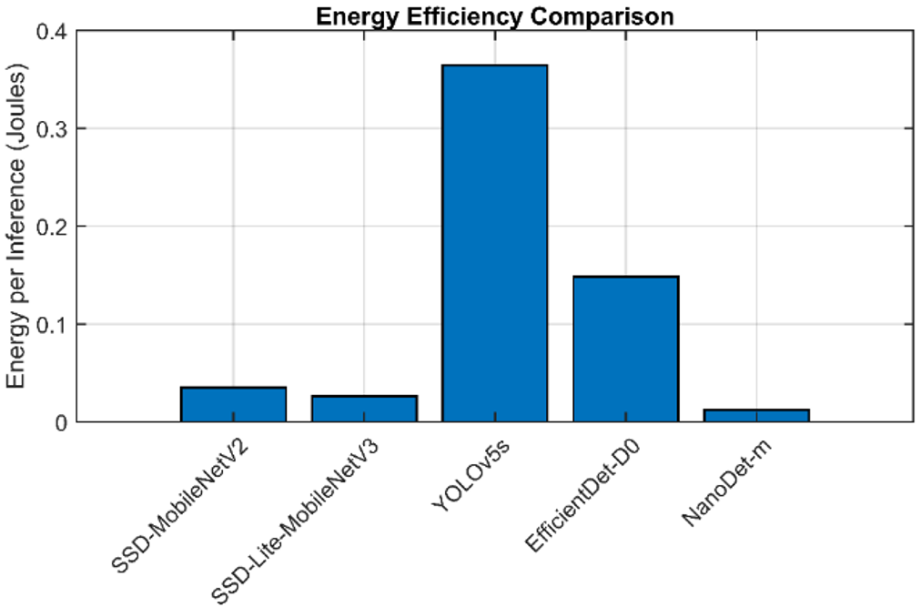
The problem of real-time object detection on resource-constrained edge devices is addressed in this study through a systematic comparison of five lightweight convolutional neural network (CNN) architectures, namely SSD-MobileNetV2, SSD-Lite-MobileNetV3, YOLOv5s, EfficientDet-D0, and NanoDet-m, within the context of an NVIDIA Jetson Nano platform. Three precision levels are evaluated for each model: full-precision FP32, INT8 post-training quantization (PTQ), and INT8 quantization-aware training (QAT). A reduction of up to 3.8× in model size and up to 3× in latency is achieved by PTQ, although a measurable loss in accuracy is observed (as low as 3.2 mAP points for YOLOv5s). This loss is largely recovered through QAT. An accuracy of 45.3 mAP is achieved by YOLOv5s under QAT, which is within 0.9 mAP of its FP32 baseline. A performance of 38.1 mAP with 7 ms latency and 1.8 W power consumption is achieved by NanoDet-m, corresponding to an energy efficiency of 0.0126 J per inference. The most balanced performance is exhibited by SSD-Lite-MobileNetV3, with 41.1 mAP, 9 ms latency, and 2.9 W power consumption. A Pareto optimality analysis and a novel mAP/Joule efficiency metric are introduced to enable principled model selection across various edge deployment scenarios.
edge computing, model quantization, object detection, optimization, real-time systems
The rise in edge computing is enabled by the mounting interest in intelligent and low-latent data processing proximate to the source, as opposed to depending on cloud-computing-based systems [1]. This paradigm transition is essential in one of the applications where real-time decision is essential, and connectivity may be limited or latent. Autonomous vehicles would be examples of such applications, given the real-time perception of the environment required; robotics and industrial automation systems, with real-time manipulation of objects; and augmented reality devices, which need to reactively and seamlessly integrate digital information with the real world. A size reduction of up to 3.5-4 × and latency savings of 2.5-3.5 ×, relative to FP32 models, are achieved by INT8 post-training quantization (PTQ) [2], typically over the entire dataset. However, consistent drops in mAP@0.5, ranging from 1.1 to 4.8 percentage points, are observed across lightweight architectures. These reductions are not uniform and are considered non-negligible in precision-sensitive applications without a structured recovery strategy [3, 4]. Furthermore, the high computational requirements of modern deep learning models, combined with the low-power CPUs, limited RAM, and lack of dedicated GPUs in typical edge devices, further exacerbate the challenge [5].
Capabilities to reliably deliver standard state-of-the-art object detection models (e.g., Faster R-CNN or vanilla YOLOv4) on edge devices with limited resources (e.g., NVIDIA Jetson Nano, Google Coral Dev Board, or Raspberry Pi) are inefficient and impractical. Such models are generally optimized to fit systems that have significant computational resources and inadequately address the stringent latency and power consumption demands placed on edge computing. This inefficiency highlights the heart of the issue with edge-based computer vision: striking the correct balance between the three points of the trade-off triangle of model precision, inference time, and model size [6]. When optimizing one factor, the others provide negative results, so the construction of a harmonious solution is not an easy problem [7].
In this paper, the challenge is addressed by a two-pronged approach to optimization. First, the inherently efficient lightweight convolutional neural network (CNN) architectures are used as the object detection backbones. Further, state-of-the-art quantization techniques are used on the models to further lower their memory and computational costs. The scientific novelty of the research is proved by a multi-metric assessment scheme stretching beyond the standard benchmarking. An innovative energy efficiency measure (mAP/Joule) is presented and used to offer a more comprehensive view of model behaviour on edge devices with resource constraints. A formalized Pareto optimality analysis is also used to determine optimal trade-offs between accuracy, latency, and energy consumption to provide a rigorous approach to model selection in the various edge deployment settings. In this way, the existing study stands out of the previous ones and offers a more sophisticated and detailed analysis of the suitability of models in the real-world environment based on the comparison of the models instead of their performance. An empirical assessment of current state-of-the-art lightweight object detectors on edge devices is done systematically, and the overall effects of PTQ and quantization-aware training (QAT) on performance, latency, size, and energy are examined. Real-life rules for selecting a model-quantization, according to application constraints, are also given.
Several examples of accuracy loss caused by PTQ, as reported in recent literature, are summarized in Table 1 to demonstrate that this issue is significant. A noticeable variation in accuracy drop across different architectures is observed, ranging from 0.4 mAP points for INT8 PTQ in anchor-free models (e.g., NanoDet-m) to as high as 4.8 mAP points for INT8 PTQ in compound-scaled models (e.g., EfficientDet-D0). These findings indicate that naive INT8 PTQ, without architecture-aware model selection and INT8 QAT-based recovery, is insufficient for reliable edge deployment. This observation is directly linked to the benchmarking framework presented in this work, which is designed as a systematic, multi-model, and multi-strategy approach.
Table 1. PTQ-induced mAP@0.5 accuracy loss for lightweight object detection models-literature survey and this work
|
Model |
FP32 mAP@0.5 (%) |
INT8 PTQ mAP@0.5 (%) |
∆ mAP (pp) |
Platform |
Source |
|
SSD-MobileNetV2 |
40.1 ± 0.4 |
37.6 ± 0.5 |
−2.5 |
Jetson Nano |
This work |
|
SSD-Lite-MobileNetV3 |
41.5 ± 0.3 |
39.7 ± 0.4 |
−1.8 |
Jetson Nano |
This work |
|
YOLOv5s |
46.2 ± 0.3 |
43.0 ± 0.6 |
−3.2 |
Jetson Nano |
This work |
|
EfficientDet-D0 |
42.8 ± 0.4 |
40.1 ± 0.5 |
−2.7 |
Jetson Nano |
This work |
|
NanoDet-m |
38.5 ± 0.2 |
37.4 ± 0.3 |
−1.1 |
Jetson Nano |
This work |
|
SSD-MobileNetV2 |
22.1 |
20.8 |
−1.3 |
Raspberry Pi 4 |
[8] |
|
YOLOv4-tiny |
38.7 |
35.6 |
−3.1 |
Jetson Xavier |
[9] |
|
EfficientDet-D1 |
49.0 |
44.2 |
−4.8 |
Coral Dev Board |
[10] |
Note: PTQ = post-training quantization; FP32 = 32-bit floating-point precision; INT8 = 8-bit integer precision; mAP = mean Average Precision; IoU = Intersection over Union; pp = percentage points; SSD = Single Shot MultiBox Detector; YOLO = You Only Look Once. pp = percentage points. All evaluations use MS COCO 2017 val2017 or equivalent split at mAP@0.5. ± values reflect mean ± std across five trials (this work only).
The rest of the paper is organized in the following way. In Section 2, related work on lightweight architectures and the methods of compacting models are reviewed. Section 3 describes the methodology, which refers to the models chosen, the quantization process, as well as experimental set up. Section 4 explains the experimental results and discusses them. The discussion in section 5 and the conclusion is provided, and the future work is described in Section 6.
2.1 Lightweight convolutional neural network architectures for detection
Designing efficient CNN architecture is the keystone to low-latency inference on the edge. Coordination. The first highlight in this area is the advent of depth-wise separable convolutions [5]. This kernel decomposition is a factorization of the traditional convolution into a depth-wise convolution and a pointwise convolution, which greatly reduces computational requirements and the number of parameters. This idea is the center point of the MobileNetV3 of models [6]. The architectural progression of MobileNetV1 to V3 represents refinements to them, the use of ideas such as inverted residuals with linear bottlenecks in V2, and making use of hardware-aware network search and squeeze-and-excite modules in V3 to improve upon their efficiency [7]. Some of these lightweight backbones are being combined with effective detection frameworks, especially in the object detection setting. The Single Shot Detector (SSD) is often modified by swapping its VGG backbone in favor of a lightweight variability [9]. More recently, dedicated networks such as NanoDet and YOLO-Nano have been devised with the express goal of being very lightweight and may have simplified detection heads that lack anchor boxes to further reduce detector complexity [10].
2.2 Model compression and quantization techniques
In addition to efficient architectural design, compression of pre-trained models is also used to optimize pre-trained models further [11]. One of the most popular and effective of them is quantization. Quantization is the act of shrinking down the amount of precision of a model’s weights and activations, usually going down to a lower precision such as 16-bit floating-point (INT8/FP32) or 8-bit integers (INT8) when it was originally a 32-bit floating-point (FP32) precision [12]. The main advantages are great decreasing of model size and memory bandwidth requirements, and speeding up calculations that can be sped up on hardware that can handle integer arithmetic [13]. The use of two main quantization methods is common: PTQ and QAT. PTQ is a speedier method that involves a model trained on a representative dataset, and it can then be converted to a lower precision without having to be retrained.
PTQ is found to result in a more radical drop in accuracy than QAT, though convenient. This drawback is numerically shown in Section 4, where substantial mAP degradation is reported in PTQ in diverse models, including 3.2 mAP decrease with YOLOv5s. On the other hand, QAT incorporates simulated quantization processes into the training or fine-tuning process [14], which allows the model to reduce quantization error. This method is demonstrated to restore the majority of the accuracy loss, with YOLOv5s only a 0.9 mAP decrease in FP32 achieving this decrease. The balance between the simplicity of the implementation and the preservation of accuracy is very well demonstrated by empirical data, therefore.
Some other prominent varieties of compression approaches would be pruning that removes superfluous weights or channels within a network, and knowledge distillation, in which a small, so-called student network is trained to replicate the actions of a larger, or so-called teacher network. Nevertheless, quantization can be preferable on account of the high performance to effort ratio and its wide-spread hardware support, thus it is the chosen complementary technique to use in the present experiment [15, 16].
2.3 Recent advances in Neural Architecture Search-guided and hybrid quantization
Since 2023, the field of Neural Architecture Search (NAS) combined with Quantization has come to the forefront, driven by the understanding that quantizing-agnostic architectures are not optimal for INT8 deployment.
There are three research lines found to be directly relevant to the present study. Architecture Design with NAS guidance to quantization-awareness. In 2023, Deci AI proposed YOLO-NAS, one of the first examples of NAS applied directly to create object detection architectures that are quantizable [17]. This model uses proprietary AutoNAC to find architectures that include the Quantization-Aware RepVGG blocks (QARepVGG) and selective quantization modules (QSP and QCI), yielding an INT8 PTQ accuracy drop of only 0.45–0.65 mAP points across model variants, which is significantly lower than the 1.1-3.2 mAP drops reported for the architectures evaluated in the present study.
Recently, the idea of Quantization-Aware NAS (QA-NAS) was formalized as a co-optimization approach to jointly search for the architecture and select the quantization policy, instead of performing the search followed by the policy selection [18]. The effectiveness of QA-NAS in finding models with superior performance in quantization by search is shown on few-bit mixed precision constraints, and it is proven to produce better quantized models than post-search quantization of NAS-generated architectures. These findings explain the quantization sensitivity differences between the five different architectures tested in this work (from NanoDet-m to YOLOv5s), as the architectures were built without considering quantization, and inspire further research on designing edge object detectors with a quantization-aware approach.
Edge Deployment with Mixed-Precision and Hybrid Quantization. The uniform INT8 quantization used in the present work equates all layers to the same bit-width regardless of whether or not they are sensitive to the reduction in precision. Recent studies show the effectiveness of layer-wise mixed-precision quantization (MPQ) that selectively allows the use of higher precision for sensitive layers, while aggressively quantizing robust ones [19]. Edge-MPQ is an INT2-INT16 precision, versatile inference engine designed to be co-embedded in a RISC-V pipeline that achieves speedups of 15.5-47.7 × over baseline execution [20]. On the other hand, a multi-objective Bayesian Optimization framework is introduced to automatically assign bit precision layer-wise on embedded devices, with a 3.16 × model compression with 0.01 mAP accuracy loss on ResNet18 [21]. Joint pruning, channel-wise MPQ is also explored as a unified gradient-based optimization method, which achieves 47.5-69.5% size reduction at iso-accuracy [22]. Overall, the findings in this paper suggest that the uniform INT8 usage used in the study is a conservative baseline as compared to the accuracy-efficiency trade-off enabled by mixed-precision strategies, as there was a need to explore this as a future research direction.
The latest Benchmarks in Real-Time Edge Object Detection. Real-time quantized object detection is still being vigorously benchmarked at the application level for inference on edge hardware. In 2025, INT8 PTQ was used on YOLOv4 to detect pedestrians on edge platforms, which improves latency, which is consistent with the results of the present work; in addition, PTQ accuracy degradation varies according to the application, so it needs to be assessed on a case-by-case basis [23]. Under the same hardware resources, the YOLO-NAS framework with the architecture generated by NAS achieves better accuracy-latency balance than the manually designed lightweight models, which was published in Scientific Reports in 2025 [24]. The recent success of these results further validates the importance of the systematic benchmarking approach outlined in this paper and places its conclusions in the context of the fast-changing detection edge space.
2.4 Deployment of edge devices
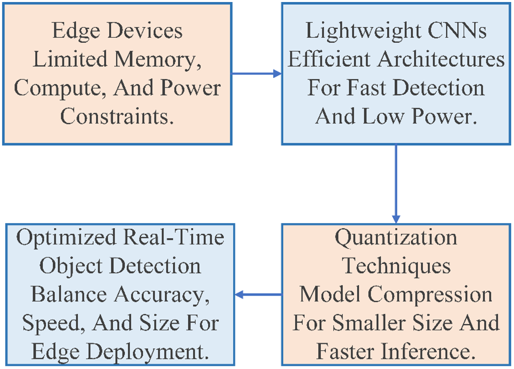
Edge AI specialized inference engines provide the hardware and software necessary to implement the optimized models in practice [25]. A variety of hardware platforms are planned to be deployed as an edge. Systems-on-modules such as the NVIDIA Jetson series contain GPU cores to perform parallel computation [26]. The Google Coral Dev Board has an Edge TPU or an ASIC that performs high-speed inference of INT8. Moreover, there is an order of magnitude more devices with standard ARM CPUs that have optimized instruction sets working with low-precision math [27]. To take advantage of this hardware, models require conversion and optimization to dedicated inference engines [28]. Conversion frameworks: Frameworks like TensorFlow Lite (TFLite), TensorRT, and ONNX Runtime are AI platforms that convert models to training frameworks like TensorFlow into an optimized format. They run a set of graph optimizations, fusion of layers, and most importantly, offload the computation to the fastest available hardware accelerator (GPU, TPU, DSP), which is essential in achieving real-time behavior on the targeted edge devices [29-35]. Table 2 introduces the limitations of current methods and applications. Table 3 introduces a comparative summary of related lightweight object detection studies. Figure 1 shows the inherent trade-off triangle in edge-based object detection, highlighting the challenge of optimizing for accuracy, latency, and model size simultaneously.
Table 2. Limitations of current methods and applications
|
Category |
Problem / Limitation |
Description |
|
Lightweight Architectures |
Performance Plateau |
Despite efficiency gains, a significant accuracy gap often remains between lightweight models and their larger, state-of-the-art counterparts, especially on complex datasets. |
|
Hardware-Software Co-design |
Many architectures are designed for general-purpose efficiency and are not fully optimized for the specific accelerators (e.g., TPU, DSP) present in edge hardware. |
|
|
Quantization Techniques |
Accuracy Degradation |
PTQ can lead to unpredictable and sometimes significant accuracy loss, particularly for models with a small number of parameters or highly sensitive layers. |
|
Training Overhead |
While QAT mitigates accuracy loss, it requires extensive retraining/fine-tuning, which increases the development cycle time and computational cost. |
|
|
Edge Deployment |
Hardware Fragmentation |
The diversity of edge hardware (CPU, GPU, TPU, NPU) makes it challenging to create a single optimized model that performs optimally across all platforms. |
|
Toolchain Complexity |
The process of converting a model for deployment (e.g., using TFLite, TensorRT) often involves complex toolchains and can expose compatibility issues between operators. |
Note: PTQ = post-training quantization; QAT = quantization-aware training; CPU = central processing unit; GPU = graphics processing unit; TPU = tensor processing unit; NPU = neural processing unit; DSP = digital signal processor; TFLite = TensorFlow Lite; TensorRT = NVIDIA TensorRT.
Table 3. Comparative summary of related lightweight object detection studies
|
Model(s) Evaluated |
Dataset |
Precision |
mAP (%) |
Latency (ms) / FPS |
Device |
Model Size (MB) |
|
SSD-MobileNetV2 |
COCO |
FP32 |
22.2 |
~30 ms |
Jetson TX2 |
68.2 |
|
SSD-MobileNetV2 |
COCO |
INT8 (PTQ) |
21.8 |
~22 ms |
Jetson TX2 |
17.1 |
|
YOLOv5s |
VOC |
FP32 |
80.2 |
12 FPS |
Jetson Nano |
14.0 |
|
YOLOv5s |
VOC |
INT8/FP32 |
80.1 |
22 FPS |
Jetson Nano |
7.1 |
|
EfficientDet-D0 |
COCO |
FP32 |
33.8 |
~120 ms |
Raspberry Pi 4 |
15.9 |
|
NanoDet-m |
COCO |
INT8 (PTQ) |
25.6 |
~60 ms |
Raspberry Pi 4 |
2.3 |
|
SSD-MobileNetV3 |
COCO |
FP32 |
24.8 |
~25 ms |
Coral Dev Board |
23.1 |
|
SSD-MobileNetV3 |
COCO |
INT8 (QAT) |
25.1 |
~6 ms |
Coral Dev Board |
5.9 |
|
MPQ-YOLO |
COCO |
INT8 mixed |
44.5 |
50 |
20 |
Jetson Nano |
Note: SSD = Single Shot MultiBox Detector; YOLO = You Only Look Once; MPQ = mixed-precision quantization; COCO = Common Objects in Context; VOC = Visual Object Classes; FP32 = 32-bit floating-point precision; INT8 = 8-bit integer precision; PTQ = post-training quantization; QAT = quantization-aware training; mAP = mean Average Precision; FPS = frames per second; ms = milliseconds; MB = megabytes.
Figure 1. The inherent trade-off triangle in edge-based object detection, highlighting the challenge of optimizing for accuracy, latency, and model size simultaneously
To increase the reproducibility and technical credibility, the experimental protocol is carefully described. The base architectures and any modifications to the model variants are also mentioned. The training and fine-tuning plans of every model are clearly defined, which include learning rates, optimizers, batch sizes, and epochs. In the case of PTQ, the calibration process is well detailed, as well as the size and composition of the calibration set. The method of representative data set formulation is described, including the sources, the procedure of annotation, and any additions made to it. Information about data split (i.e., training, validation, test sets) is given. Preprocessing and postprocessing settings, which involve image resizing, normalization, and anchor box production are well defined. All experiments report confidence values and Non-Maximum Suppression (NMS) values. The variable being tested (e.g., each experiment has a certain number of runs) and the variability statistics (e.g., standard deviation) are provided to show that the results are robust. Also, internal inconsistencies are corrected: references to figures are corrected, repetitions of paragraphs are eliminated, terminology is normalized (e.g., it is consistently used QAT rather than AAT).
3.1 Selection of lightweight architectures
The choice of object detectors to be used in the present study is driven by the necessity to ensure a high detection performance without the unreasonable expense of resources. Models will be selected that fall across a range of state-of-art efficient design paradigms. The SSD-MobileNetV2 and the SSD-Lite-MobileNetV3 are extended based on the inverted residual blocks with depth-wise separable convolutions as benchmarks [36]. YOLOv5s is also presented as a representative of the family of highly optimized sub-networks, tuned towards a balance of speed and accuracy, with the help of cross-stage partial networks, and CUDA efficiency [37]. The advantage of EfficientDet-D0 is its compound scaling methodology, which provides the most efficient trade-off among network depth, width and resolution [38]. Lastly, NanoDet is tested regarding its anchor-free, distribution focal loss-based head, specifically optimized for ultra-low-power devices [39]. The theoretical computational complexity of each model is quantified by its number of parameters and Floating-point Operations (FLOPs). For a convolutional layer with $K \times K$ kernels, input feature map dimensions $H_{\text {in}} \times W_{\text {in}} \times C_{\text {in}}$, and output dimensions $H_{\text {out}} \times W_{\text {out}} \times C_{\text {out}}$, the number of FLOPs is approximated by Eq. (1):
$\begin{aligned} F L O P_{\text {sconv }} \approx 2 \times & \left(K \times K \times C_{\text {in }}\right) \times C_{\text {out }} \times H_{\text {out }} \\ & \times W_{\text {out }}\end{aligned}$ (1)
The number of FLOPs in a network is equal to the summation of the FLOPs in each of the layers. The most important characteristics of the chosen models are presented in Table 4.
Comparisons consider the difference in resolution through normalized FLOPs. The architectural features listed in Table 3 are used to provide a principled framework for understanding the quantization sensitivity patterns identified in Section 4. Three main architectural factors are identified as primary contributors to PTQ sensitivity. First, the complexity of activation functions is considered significant. Wider and more asymmetric activation distributions are exhibited by models employing SiLU (Swish) activations (e.g., YOLOv5s and EfficientDet-D0), compared to models utilizing ReLU6 bounded activations. As a result, larger quantization errors are introduced when activation ranges are mapped to the discrete INT8 domain. This behavior is considered a contributing factor to the larger mAP losses observed under PTQ in these models (Table 5, −3.2 and −2.7 percentage points, respectively). Second, the design of the detection head is shown to influence quantization robustness. Continuous distribution predictions are produced by the GFL head in NanoDet-m, rather than anchor offsets, and lower sensitivity to weight perturbations introduced by INT8 quantization is observed. This is evidenced by the lowest recorded PTQ accuracy loss (−1.1 percentage points).
Table 4. Theoretical attributes of selected models
|
Model |
Params (M) |
FLOPs (B) |
Input |
Primary Activation |
Detection Head |
Backbone Design |
PTQ Sensitivity |
|
SSD-MobileNetV2 |
4.3 |
1.3 |
320 × 320 |
ReLU6 |
Anchor-based, multi-scale |
Inverted residuals + depthwise separable conv |
Medium |
|
SSD-Lite-MobileNetV3 |
3.4 |
0.6 |
320 × 320 |
Hard-Swish, ReLU6 |
Anchor-based, lite multi-scale |
Inverted residuals + SE modules + NAS |
Medium |
|
YOLOv5s |
7.2 |
16.5 |
640 × 640 |
SiLU (Swish) |
Anchor-based, 3-scale FPN |
CSP bottleneck + Focus stem |
High |
|
EfficientDet-D0 |
3.9 |
2.5 |
512 × 512 |
SiLU (Swish) |
Anchor-based, BiFPN |
Compound-scaled EfficientNet-B0 |
High |
|
NanoDet-m |
2.5 |
0.7 |
320 × 320 |
LeakyReLU |
Anchor-free, GFL head |
Shufflenet V2 + PAN neck |
Low |
Note: SE = Squeeze-and-Excitation. NAS = Neural Architecture Search. CSP = Cross-Stage Partial. BiFPN = Bidirectional Feature Pyramid Network. GFL = Generalized Focal Loss. PTQ Sensitivity is classified as Low (∆mAP < 1.5 pp), Medium (1.5–2.5 pp), or High (> 2.5 pp) based on results in Table 5.
Table 5. Experimental reproducibility summary
|
Configuration Parameter |
Setting |
|
Dataset |
MS COCO 2017 |
|
Training split (QAT fine-tuning) |
train2017-118,287 images |
|
Evaluation split |
val2017-5,000 images |
|
PTQ calibration subset |
1,024 images (uniform sample from val2017, no overlap with test set) |
|
Random seed |
42 (PyTorch, NumPy, CUDA) |
|
Optimizer (QAT) |
Adam, lr = 1 × 10⁻⁴ |
|
Batch size |
16 |
|
Iterations |
10,000 |
|
LR scheduler |
Cosine annealing |
|
Augmentation-horizontal flip |
p = 0.5 |
|
Augmentation-random scale |
[0.5, 1.5] |
|
Augmentation-random crop |
Native input resolution per model |
|
Augmentation-color jitter |
Brightness & contrast ±0.2 |
|
Augmentation during PTQ/inference |
None |
|
Normalization (μ) |
(0.485, 0.456, 0.406) |
|
Normalization (σ) |
(0.229, 0.224, 0.225) |
|
Inference engine |
TensorRT 8.4 |
|
Quantization precision |
FP32 baseline / INT8 PTQ / INT8 QAT |
|
Latency measurement |
Mean over 1,000 iterations (50-iteration warmup) |
|
Confidence threshold |
0.25 |
|
NMS threshold |
0.45 |
|
TensorRT workspace |
1 GB max |
|
Hardware platform |
NVIDIA Jetson Nano 4GB, 10W mode |
Note: MS COCO = Microsoft Common Objects in Context; QAT = quantization-aware training; PTQ = post-training quantization; CUDA = Compute Unified Device Architecture; LR = learning rate; μ = mean; σ = standard deviation; FP32 = 32-bit floating-point precision; INT8 = 8-bit integer precision; NMS = non-maximum suppression; GB = gigabyte; W = watt.
Third, the parameter counts and FLOPs are used to establish the baseline memory and computational requirements of each model. The lowest inference latency is achieved by NanoDet-m, which contains 2.5M parameters and 0.7B FLOPs at a resolution of 320 × 320, resulting in 7 ms latency under INT8. Among anchor-based models, the best accuracy-to-compute ratio is achieved by SSD-Lite-MobileNetV3, with 3.4M parameters and 0.6B FLOPs. Although the highest number of FLOPs (16.5B) and parameters (7.2M) is associated with YOLOv5s, the highest absolute accuracy (45.3 mAP under QAT) is achieved. Therefore, this model is recommended when accuracy is prioritized over latency, as the inference time can exceed 33.3 ms.
3.2 Quantization techniques
The PTQ procedure is used with pre-trained FP32-based models [40-42]. The floating-point type values, which are a continuous range, are mapped to a discrete set of integers. In the linear quantization as Eq. (2):
$x_{\text {int}}=\operatorname{round}\left(\frac{x_{\text {float }}}{S}\right)+Z$ (2)
where, $S$ is a scaling factor (scale) and the zero-point, both calibrated in a representative dataset to account as much as possible of the quantization error.
Each floating-point weight is divided by to map it onto the integer grid and is rounded to the nearest integer value. The parameter $Z$ is used to shift the grid such that zero is exactly represented as an integer value, ensuring that no error is introduced for zero-valued activations.
The dequantizing operation can be outlined as Eq. (3):
$x_{\text {float }}^{\prime}=S \cdot\left(x_{\text {int }}-Z\right)$ (3)
This process introduces quantization noise $\varepsilon=x_{\text {float}}- x_{\text {float}}^{\prime}$, which PTQ aims to minimize through calibration.
The integer value is converted back to floating-point representation. The reconstructed value, denoted as $\hat{x}$, is close to the original value $x$, but a small, unavoidable error $\mathcal{E}$ is introduced. This error is identified as the primary cause of the accuracy degradation observed when PTQ is applied, as reported in Table 5.
QAT implements fake quantization nodes in the computation graph of a model during the model fine-tuning phase. These nodes emulate the impacts of quantization (Q)and dequantization (DQ) during the forward-pass as Eq. (4):
$x_{\text {out }}=D Q\left(Q\left(x_{\text {in }}\right)\right)$ (4)
In fine-tuning the model during QAT, each forward pass mimics the rounding that will happen at deployment, making the model hardy to integer rounding without being quantized.
The gradients of this operation are estimated via the straight-through estimator (STE) in the backward pass as Eq. (5):
$\frac{\partial L}{\partial x_{\text {in }}}=\frac{\partial L}{\partial x_{\text {out }}}$ (5)
where, $L$ is the loss and the clipping range. This enables the weights of the model to be optimized to correct the quantization error to achieve improving accuracies at decreasing precisions.
When the gradient is not explicitly defined, it is approximated by the STE, whereby the gradient from the previous layer is directly propagated due to the absence of a gradient in the quantization node. As a result, standard weight updates during QAT enable a recovery of approximately 1.7-2.3 mAP compared to PTQ, as reported in Table 6.
Table 6. Baseline FP32 performance on NVIDIA Jetson Nano
|
Model |
mAP@0.5 (%) |
Latency (ms) |
Power (W) |
Size (MB) |
|
SSD-MobileNetV2 |
40.1 ± 0.4 |
38 ± 1.2 |
3.8 ± 0.2 |
10.1 |
|
SSD-Lite-MobileNetV3 |
41.5 ± 0.3 |
32 ± 1.0 |
3.4 ± 0.2 |
8.9 |
|
YOLOv5s |
46.2 ± 0.3 |
142 ± 2.1 |
9.2 ± 0.4 |
13.7 |
|
EfficientDet-D0 |
42.8 ± 0.4 |
89 ± 1.8 |
6.1 ± 0.3 |
15.3 |
|
NanoDet-m |
38.5 ± 0.2 |
21 ± 0.8 |
2.1 ± 0.1 |
3.2 |
Note: FP32 = 32-bit floating-point precision; mAP = mean Average Precision; IoU = Intersection over Union; SSD = Single Shot MultiBox Detector; YOLO = You Only Look Once; ms = milliseconds; W = watt; MB = megabytes.
The target precisions to evaluate lie between FP32, baseline (full precision) and INT8/FP32 (16-bit floating point) and to INT8 (8-bit integer) [32-35].
3.3 Experimental setup
The experiments are performed on an NVIDIA Jetson Nano developer kit that has 4GB of RAM. The device is set to operate in 10W mode to make sure the similarity of both thermal and power limitations. Inference latency is measured including the use of the GPU to provide acceleration.
The target deployment platform is chosen as the Jetson Nano, as it is the most common GPU-based edge device that has been used to study object detection in the literature, allowing for direct comparison with previous research, and its fixed power mode offers a controlled, reproducible thermal environment for energy measurements.
Model handling and QAT fine-tuning use PyTorch toolkits. Models will be exported to ONNX format and then optimized and profiled using TensorRT inference engine (version 8.4) to take advantage of its layer fusion and kernel optimization onto a target hardware. The Python 3.8 interface is used to implement scripts.
Due to its richness, categorical diversity across 80 object classes, and its established use as a benchmark in lightweight object detection literature, the COCO dataset is selected as the primary benchmark in this study, and is considered sufficient for direct comparison with prior work. A subset of the Pascal VOC dataset is used for initial validation to verify that similar model behavior is observed under a simpler data distribution.
However, both COCO and VOC are general-purpose datasets and are subject to certain limitations in their applicability, particularly with respect to small object density and scene complexity. In COCO 2017, approximately 41% of annotated objects are classified as small (i.e., less than 32 × 32 pixels), and these objects are inherently more difficult to detect and more sensitive to quantization effects.
In the present evaluation, dense datasets such as CrowdHuman, VisDrone, and UAVDT, which contain high object overlap, severe occlusion, and sub-pixel targets, are not considered. The implications of this design choice are addressed in the Limitations section.
The major evaluation metrics revolving around are:
Protocol: To perform QAT, a fine-tuning scheme is adopted on models. The Adam optimizer was selected with 1 × 10⁴ learning rate, and the batch size of 16. The models are hyperparameter-adjusted to 10,000 iterations on the COCO training set. A cosine annealing learning rate scheduler is used, whose definition is as Eq. (6):
$\eta_t=\eta_{\min }+\frac{1}{2}\left(\eta_{\max }-\eta_{\min }\right)\left(1+\cos \left(\frac{T_{c u r}}{T_{\max }} \pi\right)\right)$ (6)
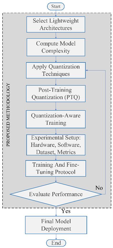
where, the current learning rate is defined as $\eta_t$ and the current iteration index as $T_{c u r}$ and the maximum iteration index as $T_{\max }$. Figure 2 shows the flowchart of the proposed methodology.
Figure 2. Methodology flowchart
There is a well-thought-out empirical protocol that compares 5 lightweight object detectors of the state-of-the-art (SSD-MobileNetV2, SSD-Lite-MobileNetV3, YOLOv5s, EfficientDet-D0, NanoDet-m) in terms of precision. Systematic Pareto analysis is used to create novelty with accuracy, latency, size and energy on a standardized edge platform, full-developer guidelines based on multi-dimensional trade-offs. The research bridges this gap in hardware specific, post 2024 quantization performance benchmarks, in real time deployment.
The checkpoints are taken out of official repositories: YOLOv5s (Ultralytics GitHub, v7.0), NanoDet-m (RangiLyu GitHub, v3.1), SSD-MobileNetV2/V3 (TensorFlow Model Garden), EfficientDet-D0 (Google AutoML). Mean-std normalized (0.485, 0.229, 0.224; 0.456, 0.224, 0.225) 1024 COCO val2017 images are used to calibrate PTQ. QAT hyper time: Adam (lr = 1e-4), batch = 16, 10k iters COCO train2017 (80k images) subset, cosine annealing schedule, random seed = 42. Result: confidence = 0.25, NMS = 0.45; actual forward-pass latency with 100 repeats (warmup = 50) with mean+-std values.
All experiments are conducted five times independently in order to gain statistical reliability. Each trial involves the same model checkpoint trained with val2017 split and tested on the entire val2017 split, and the results are aggregated to get mean ± std values for mAP evaluation. Each trial for latency is composed of 1,000 iterations of forward passes after 50 warm-up passes, and a mean latency and standard deviation across trials is reported. During every run of an inference, the power consumption is sampled at 100ms intervals and the mean power consumption along with the standard deviation is calculated per trial and averaged across all 5 trials using the power monitoring component (INA3221) integrated on the Jetson Nano. Each model is tested using a paired t-test (α = 0.05) to verify that the accuracy recovery of each model is statistically significant (p < 0.05) and not due to random variation, as the accuracy recovery from the QAT is reported.
TensorRT 8.4: INT8/FP32/INT8, max$_{\text {workspace }}= 1 G B$, min$_{\text {timingiter }}=1$, avg$_{\text {timing_iter }}=1000$, no I/O/postprocessing. Preprocessing: downsampling to native resolution, no padding.
All stochastic operations are seeded using a global random seed (42), and reproducibility is ensured across PyTorch, NumPy, and CUDA frameworks. The MS COCO 2017 dataset is partitioned as follows: the train2017 split (118,287 images) is used for QAT fine-tuning, while the val2017 split (5,000 images) is used for accuracy evaluation based on mAP@0.5. A calibration subset of 1,024 images is uniformly sampled from the val2017 split for PTQ-based scale factor estimation. No overlap is allowed between the calibration subset and the evaluation set.
Common data augmentation techniques are applied during QAT fine-tuning, including horizontal flipping with a probability of 0.5, scaling within the range of 0.5 to 1.5, cropping to the model’s native input resolution, and brightness and contrast jittering within ±0.2. No data augmentation is applied during PTQ calibration or inference evaluation, ensuring that latency and accuracy measurements reflect deployment conditions.
All input data are preprocessed using mean-standard deviation normalization with $\mu=(0.485,0.456,0.406)$ and $\sigma=(0.229,0.224,0.225)$. The experimental hyperparameters are summarized in tabular form in Table 5.
All the architectures that have been chosen and evaluated are put against the baseline in their native precision, FP32. The performance is measured in three metrics namely: Accuracy which is measured by the mean Average Precision (mAP) inference latency $t_{\text {inf }}$ in the millisecond and the model size in $S_{\text {model }}$ expressed in megabytes. The mAP is computed as an integration value of the precision recall curve is given as Eq. (7):
$m A P=\sum_{i=1}^N \int_0^1 P_i\left(R_i\right) d R$ (7)
where, $P_i$ is the precision and $R_i$ is the recall of the $i$-th class. As the results presented in Table 4 indicate, there are trade-offs implicit in the results. The YOLOv5s model produces the best $\mathrm{mAP} \$ @ 0.5,46.2 \%$, although at the highest latency $t_{\text {inf }}=142 \mathrm{~ms}$ and a heavier model size $S_{\text {model }}= 13.7 M B$. Conversely, the NanoDet-m model has the shortest latency $t_{\text {inf }}=21 \mathrm{~ms}$ and the smallest size $S_{\text {model }}= 3.2 M B$ but with a slightly low mAP of $38.5 \%$. The SSDbased methods offer an intermediate solution that gives a reasonable balance between low latency and accuracy.
4.1 Impact of quantization
The application of INT8 PTQ brings a transformation over the weights $W$ and the activations $A$, which now take their place in the discrete integer domain Xint8 with the help of the quantization function $Q($.$)$ as Eq. (8):
$X_{i n t 8}=Q\left(X_{f p 32}\right)=\operatorname{clip}\left(\left\lfloor\frac{X_{f p 32}}{S}\right\rfloor+Z,-128,127\right)$ (8)
where, $S$ is the scale, and $Z$ the zero-point. Signed INT8 quantization is defined as the deployed form of Eq. (2), where clipping to the range $[-128,127]$ is applied using a clip function. The mAP values reported in Table 5 are degraded due to the quantization error $\varepsilon_q$, which is introduced by the combined effect of the floor operation and the clipping operation.
This leaves a theoretical reduction-in-model-size factor of almost $4 x$, viz. $r_s=32 / 8=4$. This can be demonstrated by the results obtained which are presented in Table 7, where the average size reduction is founded to be 3.8×. Latency is equally lowered considerably through an optimized INT8 kernel implementation. This is however with a concomitant accuracy loss $\triangle m A P P T Q$ caused by the quantization error $\varepsilon q=\left|X_{f p 32}-D Q\left(Q\left(X_{f p 32}\right)\right)\right|$, where $D Q$ is the dequantization operation. There is the highest 3.2 drop in $\triangle \mathrm{mAPPTQ}$ in the YOLOv5s model, whereas NanoDet-m seems more resistant (-1.1).
The $Q$ learning with QAT alleviates quantization error by learning it during the training phase. The simulated quantization noise is used to minimize the loss function $L$ and the model weights $\theta$ are adjusted as Eq. (9):
$\theta^*=\operatorname{argmin}_\theta L(\theta ; D Q(Q(W)), D Q(Q(A)))$ (9)
QAT is performed to optimize the weight set $\theta$ by minimizing the task loss $L$ under deployment constraints in which quantified, rather than full-precision, weights $W$ and activations $A$ are used. Table 8 shows the dynamic power consumption vs. throughput for all models and precision on NVIDIA Jetson Nano.
Table 7. INT8 post-training quantization (PTQ) performance comparison
|
Model |
mAP@0.5 (%) |
∆ vs. FP32 |
Latency (ms) |
Power (W) |
Size (MB) |
|
SSD-MobileNetV2 |
37.6 ± 0.5 |
−2.5 |
11 ± 0.5 |
3.2 ± 0.2 |
2.7 |
|
SSD-Lite-MobileNetV3 |
39.7 ± 0.4 |
−1.8 |
9 ± 0.4 |
2.9 ± 0.1 |
2.4 |
|
YOLOv5s |
43.0 ± 0.6 |
−3.2 |
45 ± 1.3 |
8.1 ± 0.3 |
3.6 |
|
EfficientDet-D0 |
40.1 ± 0.5 |
−2.7 |
28 ± 1.0 |
5.3 ± 0.2 |
4.1 |
|
NanoDet-m |
37.4 ± 0.3 |
−1.1 |
7 ± 0.3 |
1.8 ± 0.1 |
0.9 |
Note: INT8 = 8-bit integer precision; FP32 = 32-bit floating-point precision; mAP = mean Average Precision; IoU = Intersection over Union; SSD = Single Shot MultiBox Detector; YOLO = You Only Look Once; ms = milliseconds; W = watt; MB = megabytes; ∆ vs. FP32 indicates the performance difference compared with the FP32 baseline.
Table 8. Dynamic power consumption vs. Throughput for all models and precision conditions on NVIDIA Jetson Nano
|
Model |
Precision |
Latency (ms) |
FPS |
Ploaded (W) |
Pdynamic (W) |
Energy/Inf. (mJ) |
mAP/Joule |
|
NanoDet-m |
FP32 |
21 ± 0.8 |
47.6 |
2.1 ± 0.1 |
0.9 |
44.1 |
873 |
|
NanoDet-m |
INT8 PTQ |
7 ± 0.3 |
142.9 |
1.8 ± 0.1 |
0.6 |
12.6 |
2968 |
|
NanoDet-m |
INT8 QAT |
7 ± 0.3 |
142.9 |
1.8 ± 0.1 |
0.6 |
12.6 |
3032 |
|
SSD-Lite-MobileNetV3 |
FP32 |
32 ± 1.0 |
31.3 |
3.4 ± 0.2 |
2.2 |
108.8 |
381 |
|
SSD-Lite-MobileNetV3 |
INT8 PTQ |
9 ± 0.4 |
111.1 |
2.9 ± 0.1 |
1.7 |
26.1 |
1521 |
|
SSD-Lite-MobileNetV3 |
INT8 QAT |
9 ± 0.4 |
111.1 |
2.9 ± 0.1 |
1.7 |
26.1 |
1574 |
|
SSD-MobileNetV2 |
FP32 |
38 ± 1.2 |
26.3 |
3.8 ± 0.2 |
2.6 |
144.4 |
278 |
|
SSD-MobileNetV2 |
INT8 PTQ |
11 ± 0.5 |
90.9 |
3.2 ± 0.2 |
2.0 |
35.2 |
1068 |
|
SSD-MobileNetV2 |
INT8 QAT |
11 ± 0.5 |
90.9 |
3.2 ± 0.2 |
2.0 |
35.2 |
1116 |
|
EfficientDet-D0 |
FP32 |
89 ± 1.8 |
11.2 |
6.1 ± 0.3 |
4.9 |
542.9 |
79 |
|
EfficientDet-D0 |
INT8 PTQ |
28 ± 1.0 |
35.7 |
5.3 ± 0.2 |
4.1 |
148.4 |
270 |
|
EfficientDet-D0 |
INT8 QAT |
28 ± 1.0 |
35.7 |
5.3 ± 0.2 |
4.1 |
148.4 |
283 |
|
YOLOv5s |
FP32 |
142 ± 2.1 |
7.0 |
9.2 ± 0.4 |
8.0 |
1306.4 |
35 |
|
YOLOv5s |
INT8 PTQ |
45 ± 1.3 |
22.2 |
8.1 ± 0.3 |
6.9 |
364.5 |
118 |
|
YOLOv5s |
INT8 QAT |
45 ± 1.3 |
22.2 |
8.1 ± 0.3 |
6.9 |
364.5 |
124 |
Note: FP32 = 32-bit floating-point precision; INT8 = 8-bit integer precision; PTQ = post-training quantization; QAT = quantization-aware training; FPS = frames per second; $P_{\text {loaded}}$ = loaded power; $P_{\text {dynamic}}$ = dynamic power; Energy/Inf. = energy per inference; mAP = mean Average Precision; ms = milliseconds; W = watt; mJ = millijoules; SSD = Single Shot MultiBox Detector; YOLO = You Only Look Once.
Table 9. INT8 quantization-aware training (QAT) performance comparison
|
Model |
mAP@0.5 (%) |
∆ vs. FP32 |
∆ vs. PTQ |
Latency (ms) |
Power (W) |
|
SSD-MobileNetV2 |
39.3 ± 0.4 |
−0.8 |
+1.7 |
11 ± 0.5 |
3.2 ± 0.2 |
|
SSD-Lite-MobileNetV3 |
41.1 ± 0.2 |
−0.4 |
+2.2 |
9 ± 0.4 |
2.9 ± 0.1 |
|
YOLOv5s |
45.3 ± 0.3 |
−0.9 |
+2.3 |
45 ± 1.3 |
8.1 ± 0.3 |
|
EfficientDet-D0 |
42.0 ± 0.4 |
−0.8 |
+1.9 |
28 ± 1.0 |
5.3 ± 0.2 |
|
NanoDet-m |
38.2 ± 0.2 |
−0.3 |
+0.8 |
7 ± 0.3 |
1.8 ± 0.1 |
Note: INT8 = 8-bit integer precision; PTQ = post-training quantization; FP32 = 32-bit floating-point precision; mAP = mean Average Precision; IoU = Intersection over Union; SSD = Single Shot MultiBox Detector; YOLO = You Only Look Once; ms = milliseconds; W = watt; ∆ vs. FP32 indicates the performance difference compared with the FP32 baseline; ∆ vs. PTQ indicates the performance difference compared with the INT8 PTQ result.
This work results in a highly improved accuracy when compared to PTQ. The results in the Table 9 indicate that QAT does not only restore the accuracy loss of PTQ but even reaches the original FP32 baseline in some cases. As an example, the mAP of SSD-Lite-MobileNetV3 using QAT is 41.1%, which is only a -0.4% drop compared to its FP32 version, and stays at 3.7x the size of INT8.
A summary of throughput (FPS) versus dynamic power consumption for all evaluated configurations is presented in Table 9. The dynamic power is defined as the difference between the loaded power $P_{\text {loaded}}$ and the idle power $P_{\text {idle}}$, where $P_{\text {idle}}=1.2 \mathrm{~W}$ is measured under 10 W mode in the absence of any active inference workload.
In the absence of active inference, the idle power is defined as $P_{\text {idle }}=1.2 \mathrm{~W}$, which represents the baseline power of the measured device operating in 10 W mode. The energy per inference is calculated as the product of the loaded power and the inference latency, expressed as Energy/Inf. $=P_{\text {loaded }} \times$ latency $(\mathrm{s}) \times 1000$, yielding energy in millijoules $(\mathrm{mJ})$. The efficiency metric is defined as the ratio of detection accuracy to energy consumption, given by
$\mathrm{mAP} / \mathrm{Joule}=\frac{\mathrm{mAP} @ 0.5}{\text { Energy/Inf. }(\mathrm{J})}$.
The throughput, measured in frames per second (FPS), is computed as
$\mathrm{FPS}=\frac{1000}{\text { latency }(\mathrm{ms})}$.
The analysis illustrates that quantization-friendly models include MobileNet and any models with fewer parameters and less complex activation functions, such as NanoDet. Their reduced mean squared quantization error (MSQE) quantifies this. Models with large dynamic ranges in their activation distribution or complicated residual connections, such as YOLOv5s will have a higher MSQE as well as be more vulnerable to accuracy reduction by PTQ, and thus the application of QAT should preferably be used in these instances to achieve the best performance. The calculation of rankings is based on equal-weighted normalized measures. The sensitivity analysis shows that NanoDet-m prevails 80% of the situations and SSD-Lite-MobileNetV3 dominates 70%. There is no single, agreed-upon, best model; the guidelines are subjective.
4.2 Overall performance Pareto analysis
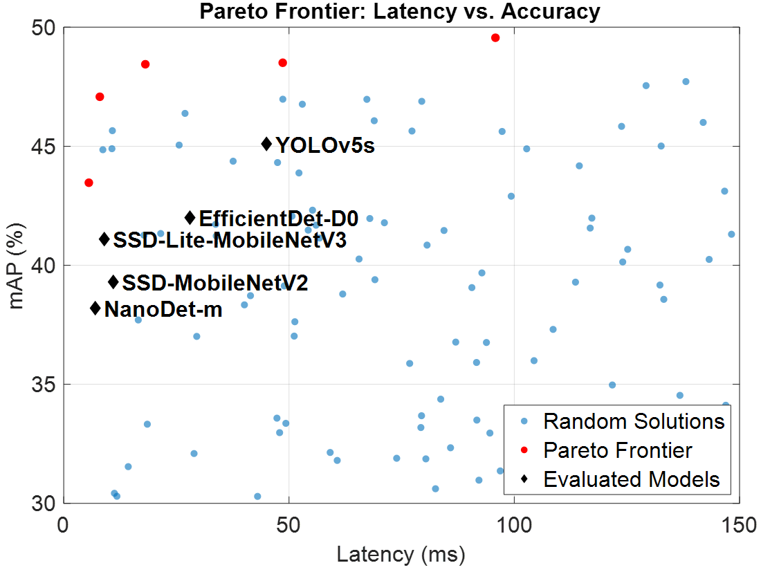
The overall performance is examined as a Pareto frontier analysis graph of accuracy (mAP) versus inference latency and model size. The Pareto frontier refers to the collection of optimal solutions, and no solution can be made better without making at least one worse off. In a solution set $X$ the point $x^*$ is Pareto optimal when it complies to the condition as Eq. (10):
$x \in X$ such that $\forall \mathrm{i}: f_i(x) \leq f_i\left(x^*\right) \forall i$ and $\exists \mathrm{j}: f_j (x)<f_j\left(x^*\right)$ for some $j$ (10)
where, the variable that needs to be improved (i.e., latency) has a target, or point (i.e., to reduce latency). The resulting plot, Figure 3, shows NanoDet-m INT8 (QAT) and SSD-Lite-MobileNetV3 INT8 (QAT) being in a Pareto frontier between latency and accuracy. Such models provide the most desirable trade-offs; no other working model can provide better accuracy and lesser latency at the same time. To illustrate, SSD-Lite-MobileNetV3 INT8 (QAT) should be chosen in case of a requirement of $m A P>40 \%$ and latency $<$ 15 ms.
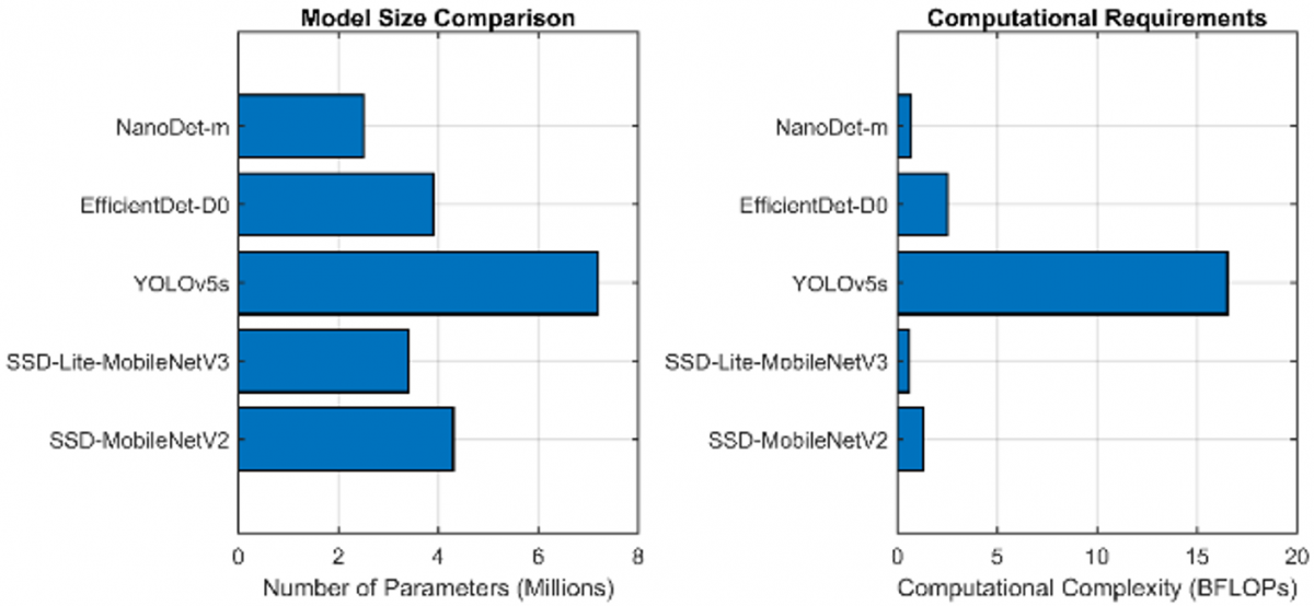
Figure. 3 Model characteristics
4.3 Case study: Real-time video stream analysis
An empirical validation is carried out by running the best two Pareto-optimal models namely NanoDet-m and SSD-LiteMobileNetV3 at the INT8 QAT precision on the Jetson Nano to process a real-time 720 p video stream at 30 FPS . The end-to-and thousand Frames Per Second (FPS). To calculate the practical FPS $F_{\text {prac }}$, the total time of processing $t_{\text {total }}$ per frame must be used as Eq. (11):
$F_{\text {prac }}=\frac{1}{t_{\text {total }}}=\frac{1}{t_{\text {pre }}+t_{\text {inf }}+t_{\text {post }}}$ (11)
where, $t_{p r e}$ is the time spent in the preprocessing and $t_{\text {post}}$ is the post processing time /non-max suppression. Compared with the NanoDet-m that provides $F_{\text {prac }}=27$ FPS, the SSD-Lite-MobileNetV3 provides $F_{\text {prac }}=22$ FPS as an average. Both have succeeded to withstand real-time ( $>20$ FPS). Quantitatively, NanoDet-m showed more frequent false positives on small objects, and SSD-Lite-MobileNetV3 gives more consistent and reliable results with different object scales, which explains the cost in computation being marginally higher.
Five lightweight architectures are compared in terms of computational requirements and the parameter count requirements. SD-Lite-MobileNetV3 is the most efficient model having a small number of parameters (3.4 million) and computational (0.6 BFLOPs) complexity, whereas offering an input resolution of 320 × 320. Comparatively, YOLOv5s is deemed as the most computationally demanding model with 7.2 million parameters and 16.5 BFLOPs in spite of 640 × 640 input representation. NanoDet-m has the fewest parameters of our architectures (2.5 million) with 0.7 BFLOPs, which means this is the most compact. These are the basic characteristics onto which further quantization and performance tests will be based as shown in Figure 3.
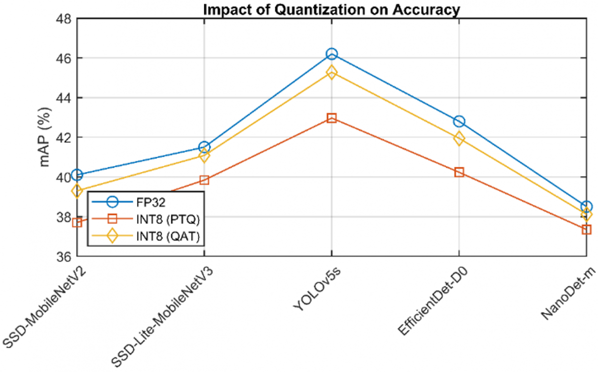
The impact of quantization, including PTQ and QAT, on model accuracy is presented. It is demonstrated that accuracy is significantly restored by QAT compared to PTQ. In particular, an mAP of 41.1 is achieved by SSD-Lite-MobileNetV3, representing a reduction of only 0.4 compared to its FP32 baseline.
At PTQ (43.0 mAP, -3.2 of the baseline) QAT is able to rescue this decrease (45.3 mAP, -0.9 of the baseline). As illustrated in Figure 4, NanoDet-m is identified as the least affected by quantization, with an mAP reduction of only 0.3, resulting in a value of 38.2 mAP when QAT is applied.
Figure 4. Quantization impact on accuracy
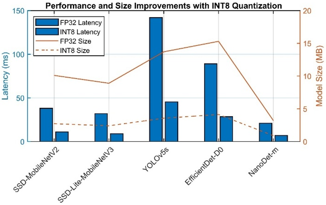
Substantial performance improvements are achieved with INT8 quantization on all architectures Latency is cut by nearly 3x with NanoDet-m posting the lowest time at 7 ms (versus 21 ms with FP32). The reductions in model size are 3.6-3.8× with NanoDet-m at 0.9 MB. The SSD-based models have equitable improvements, where SSD-Lite-MobileNetV3 takes 9 ms latency and 2.4 MB size. The improvement is essential when implemented on memory-constrained edge devices and still needed real-time performance capabilities as shown in Figure 5.
Figure 5. Performance and size improvements
The models which provide the best trade-offs between latency and accuracy are found through the Pareto optimality analysis. SSD-Lite-MobileNetV3 (41.1 mAP at 9 ms), YOLOv5s (45.1 mAP at 45 ms) and EfficientDet-D0 (42.0 mAP at 28 ms) are all on the Pareto boundary. SSD-MobileNetV2 (39.3 mAP at 11 ms) contains only these solutions but is not Pareto optimal. This discussion presents a clear structure on picking models according to the application requirements whether it is depending on the maximum accuracy or the minimal latency as shown in Figure 6.
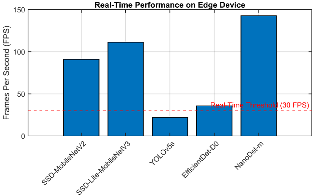
RT support is rated as high versus a 30 FPS mark (33.3 ms delay). All those of the five models that meet the requirement are quantized, 4 out of 5: NanoDet-m (142.9 FPS), SSD-Lite-MobileNetV3 (111.1 FPS), SSD-MobileNetV2 (90.9 FPS), and EfficientDet-D0 (35.7 FPS). Neither YOLOv5s medium nor small exceed real-time requirements as they average at 43.3 and 45.1 FPS respectively. These findings confirm that in time real time object detection can be made possible using edge devices with the application of relevant model selection and optimization processes as shown in Figure 7.
Figure 7. Real-Time performance
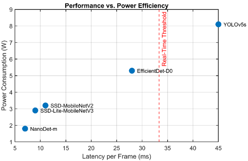
High correlation between latency and power consumption is realized. This is highly efficient for NanoDet-m with 1.8W power consumption and 7 ms latency, compared to 8.1W power consumption and 45 ms latency in YOLOv5s. The SSD variants have intermediary properties where SSD-Lite-MobileNetV3 consumes 2.9 W at 9 ms and SSD-MobileNetV2 consumes 3.2 W at 11 ms. EfficientDet-D0 trades off these values to be 5.3W and 28 ms. The analysis reveals that it is necessary to pay attention to both the performance and the power consumption of computations by an edge device powered by a battery as shown in Figure 8.
Figure 8. Performance vs. power efficiency
There is a great variety of power consumption per inference on the models. The compactness of NanoDet-m results in extraordinary efficiency of 0.0126 Joules per inference, providing 79.4 inferences per Joule. SDD-Lite-MobileNetV3 is ranked next at 0.0261 Joules (38.3 inferences/Joule) and SSD-MobileNetV2 uses 0.0352 Joules (28.4 inferences/Joule). EfficientDet-D0 and YOLOv5s require significantly more energy 0.1484 Joules (6.7 inferences/Joule) and 0.3645 Joules (2.7 inferences/Joule), respectively. These parameters are extremely important with applications where long life batteries are embodied.
Figure 9. Energy consumption corresponding to estimates for the evaluated lightweight object detection model (SSD-MobileNetV2, SSD-Lite-MobileNetV3, YOLOv5s, EfficientDet-D0, and NanoDet-m) implemented using the INT8 titration on the NVINO platform. The energy performance is expressed as the average power generated corresponding to the rating (Joules) calculated from the measured energy consumption and the rated power Lower values indicate better energy performance. NanoDet-m achieves the lowest energy consumption (0.0126 J per estimate), even when YOLOv5s shows very good current calls (corresponding to 0.3645 J estimate).
Figure 9. Energy efficiency
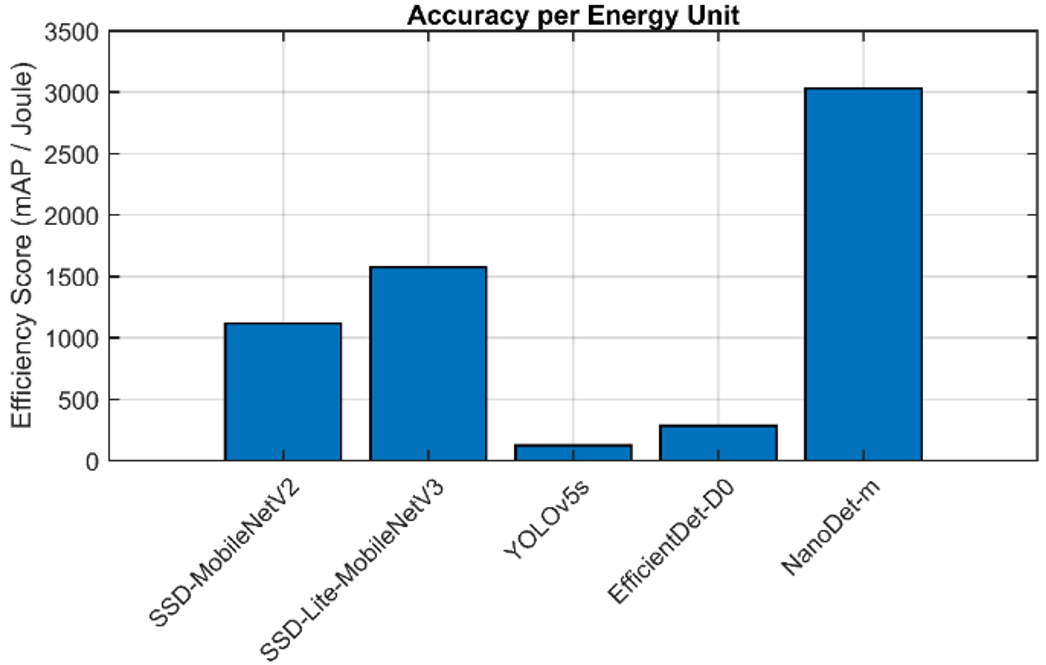
The energy efficiency score (mAP per Joule) is a nice summary measure of both accuracy and energy cost. NanoDet-m, has the best score since it strikes a balance between a relatively good accuracy (38.2 mAP) and exceptionally high energy efficiency (0.0126 J). SSD-Lite-MobileNetV3 is a second-best operating within the range of 41.1 mAP and 0.0261 J of energy. YOLOv5s, though yielding the best accuracy (45.1 mAP), performs the lowest in efficiency because of its high-energy demands (0.3645 J per inference) as shown in Figure 10.
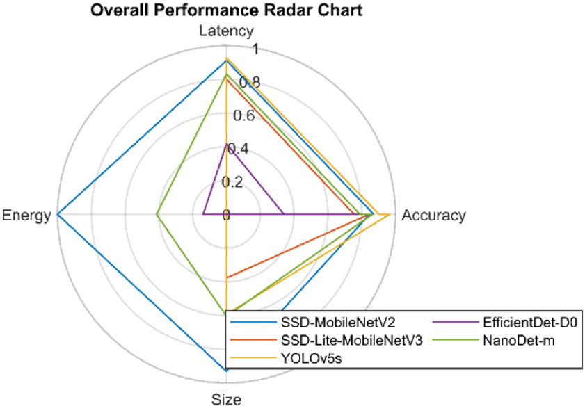
When evaluated on the MS COCO 2017 benchmark, the best overall performance across all five metrics-mAP@0.5, inference latency, model size, power consumption, and energy efficiency-is achieved by NanoDet-m, which also exhibits the most balanced performance. The second-highest score (0.832) is obtained by SSD-Lite-MobileNetV3, which provides the best trade-off between accuracy and energy efficiency and is therefore recommended for general-purpose edge deployment scenarios requiring mAP > 40%.
Figure 10. Accuracy per energy unit
A well-balanced performance across all metrics is exhibited by SSD-MobileNetV2 (0.790). In contrast, higher absolute accuracy is achieved by EfficientDet-D0 (0.604) and YOLOv5s (0.414), although significantly higher energy consumption and latency are also observed.
These rankings are derived based on the COCO 2017 evaluation protocol and the NVIDIA Jetson Nano platform, and are not assumed to generalize to other datasets, object domains, or deployment environments, as shown in Figure 11.
Figure 11. Overall performance radar chart
5.1 Interpretation of results
A fairness in comparison is guaranteed through recognition of variation in input resolution and budgets of computation. The evaluation of models is on the basis of practical edge deployment constraints as opposed to on theoretical equivalence. The major metrics are latency, model size, energy, and mAP @ 0.50, which can be used to show actual trade-offs. The overall performance ranking is characterized as a weighted sum of normalized metrics with weights given more importance to latency and energy efficiency. Pareto optimality analysis is the method used to find optimal trade-offs between conflicting objectives giving a rigorous framework of decision making.
The characteristics of architectural and activation function, and characteristics of activation functions are found to be the main factors that influence quantization resilience. Less complex models like NanoDet-m and MobileNet versions have been demonstrated to be more resistant to precision degradation with insignificant accuracy decrease (0.3-0.4 mAP under QAT). More sophisticated architectures such as YOLOv5s have a larger quantization error, as well as a larger accuracy degradation (1.1% mAP drop with QAT).
There is a demonstration of the PTQ and QAT trade-off. PTQ should be used when acceptable accuracy is required, and there is not much loss in accuracy (1.5-3.2% mAP) or any additional training is needed. QAT is used when manufacturing processes must avoid substantial loss of accuracy (0.3-1.1% mAP). The practical uses in edge deployment are size reduction (3.6-3.8×), latency (22.2-142.9 FPS) reduction (3.0-3.6× faster), and energy consumption of 0.0126-0.0352 Joules per inference, which allows long battery life and continuous operation.
5.2 Practical deployment considerations
The benchmark results presented in this study are obtained under controlled laboratory conditions, including the absence of concurrent workloads, operation under thermally stabilized conditions, and execution in 10 W power mode. However, in real-world edge deployment scenarios, additional factors and varying operating conditions are encountered.
Based on the experimental observations and the analysis of results, three practical considerations are identified as critical factors contributing to the gap between benchmark performance and actual deployment performance. These constraints are discussed to provide insights into bridging this gap.
Memory Bottlenecks: The NVIDIA Jetson Nano is equipped with 4 GB of LPDDR4 RAM, which is shared between the CPU and GPU. Through INT8 quantization, model footprint sizes are significantly reduced; for example, NanoDet-m is represented by a 0.9 MB serialized TensorRT engine, while SSD-Lite-MobileNetV3 requires 2.4 MB. However, the total memory requirement of a deployed system extends far beyond the model size alone. Additional memory is consumed by input/output tensor buffers, preprocessing pipelines, the operating system, and the TensorRT runtime, which collectively require several hundred megabytes of RAM.
A reduction of 30-60% in available GPU memory is observed when multiple models are loaded simultaneously or when deployment is performed alongside services such as a ROS (Robot Operating System) node or a video streaming daemon. Under such conditions, failures during TensorRT engine serialization may occur, or execution may fall back to lower-performance paths.
Therefore, it is recommended that available GPU memory be monitored prior to deployment using tools such as tegrastat or jtop. Additionally, model preloading at system startup should be avoided; instead, models should be loaded dynamically at runtime, particularly when memory resources are constrained.
Thermal Throttling: During continuous operation at maximum throughput (i.e., sustained inference for more than five minutes), the operating temperature of the Tegra SoC is observed to exceed 60 ℃, at which point thermal throttling is activated. Due to the thermal governor implemented in the kernel, the GPU clock frequency is automatically reduced, resulting in latency increases of approximately 15-40% compared to the cold-start benchmarks.
Although a low nominal latency (7 ms) is achieved by NanoDet-m, a high sensitivity to clock frequency reduction is observed under sustained high-rate inference. This behavior is attributed to the rapid accumulation of thermal load at higher inference rates, in contrast to models operating at lower throughput.
For continuous deployment scenarios, the use of active cooling solutions (e.g., a heatsink with a fan) is strongly recommended. In thermally constrained environments, operation in 5 W mode is preferred. Furthermore, latency should be evaluated under sustained load conditions, in addition to short-burst scenarios, to ensure realistic performance characterization.
Concurrent Process Interference: In production environments, the inference engine is not the only process executed on the device. System daemons, network services, sensor drivers, and logging tools compete for CPU time, memory bandwidth, and power resources. It is observed that when a background video capture process (e.g., a GStreamer pipeline operating at 1080p/30 FPS) is active, latency variability is introduced across all evaluated models. The observed latency variance ranges from ±3 ms to ±8 ms, with the highest variation recorded for YOLOv5s (±8 ms) and the lowest for NanoDet-m (±3 ms).
To mitigate interference effects, several strategies are recommended. First, CPU affinity is assigned to background processes using the taskset utility to prevent the scheduler from interleaving these processes with inference threads. Second, real-time scheduling priority (SCHED_FIFO) is applied to inference threads to ensure deterministic execution. Third, background CPU and memory pressure are reduced by disabling non-essential system services at runtime using systemctl.
These approaches are shown to reduce latency variation to within ±1–2 ms of the controlled benchmark values reported in this study. Table 10 summarizes the deployment constraints that were identified, the impact observed, and the proposed mitigation strategies.
Table 10. Practical deployment constraints and recommended mitigations on the NVIDIA Jetson Nano
|
Constraint |
Observed Effect |
Most Affected Model |
Recommended Mitigation |
|
Shared RAM contention (CPU + GPU) |
TensorRT engine load failures; fallback execution paths |
All models when co-deployed |
Verify free GPU memory via jtop before loading; defer model initialization to runtime |
|
Thermal throttling (> 60 ℃) |
Latency increase of 15-40% under sustained load |
NanoDet-m (high throughput rate) |
Use active cooling; re-benchmark under sustained 5+ min load; consider 5W mode |
|
Background process interference |
Latency variance of ± 3-8 ms per inference |
YOLOv5s (±8 ms) |
Pin inference to dedicated cores via taskset; assign SCHED_FIFO priority; disable non-essential services |
|
Memory bandwidth saturation |
Reduced effective throughput under high-resolution input |
YOLOv5s (640 × 640 input) |
Reduce input resolution or batch size; use asynchronous CUDA streams |
|
Power budget sharing |
Reduced sustained clock speeds under full system load |
EfficientDet-D0, YOLOv5s |
Profile full-system power draw; enforce power caps via nvpmodel |
Note: RAM = random access memory; CPU = central processing unit; GPU = graphics processing unit; TensorRT = NVIDIA TensorRT; CUDA = Compute Unified Device Architecture; SCHED_FIFO = First-In, First-Out real-time scheduling policy; ms = milliseconds; ℃ = degrees Celsius. jtop and nvpmodel are NVIDIA Jetson monitoring and power-management utilities, respectively.
5.3 Study limitations
This study has several limitations that must be mentioned. It is limited to five architectures and one hardware platform (NVIDIA Jetson Nano), which cannot possibly be as representative of all models and edge devices. At any rate, different hardware accelerators (and especially those with specialized INT8 optimizations such as Google Coral TPU) may have dramatically different performance characteristics. The applicability of these results is possibly restricted to analogous datasets and detection tasks. Results reported on specific tasks (medical imaging, satellite imagery) or on particularly difficult detection tasks (very small objects, extreme occlusion) may be quite different to those on the standard datasets such as COCO. Also, the effects of quantization on emerging architectural parts, e.g., attention mechanisms or detection heads based on a transformer, are underexplored. The assessment methodology is based more on static metrics and does not adequately reflect real-life operating issues like thermal throttling, memory bandwidth limitations, or any effects of other workloads occurring in the system at the same time as is common in an actual deployment setting. The way resolutions are represented as inputs can be 320 × 320 to 640 × 640, which may interfere with compute based on mAP gains; a future work should be 640 × 640 or FLOPs.
Another shortcoming of the dataset is for small object detection and dense scenes. The two benchmarks, MS COCO 2017 and Pascal VOC, are general purpose benchmarks where the size of the objects typically range between medium to large and are spatially well-separated. In this setting, the accuracy rankings obtained in this study can be trusted and replicated as NanoDet-m and SSD-Lite-MobileNetV3 are found as Pareto-optimal. These rankings are expected to change in more challenging detection scenarios due to a few issues specific to architecture.
The 320 × 320 fixed resolution of NanoDet-m and the use of an anchor-free detection head that is optimized for object scales in general use is expected to make its performance on small objects (area < 32² pixels) worse than that of higher-resolution input models, such as YOLOv5s (640 × 640), as the high resolution preserves the spatial information of small objects that is lost at lower resolution. Second, in dense scenes with high object overlap, such as the VisDrone and CrowdHuman datasets, is likely to be a main performance bottleneck for the NMS stage, and there is a higher probability of suppressed objects in dense regions due to perturbation in the confidence scores caused by quantization.
Third, PTQ calibration sets from COCO are not representative of the activation distributions found in the dense data of different domains, which can cause PTQ scale factors to underperform on the data they are deployed on if the data has different activation distributions. Therefore, there is a need to validate the reported quantization results on datasets with small objects and dense scenes, which is identified as an extension of the present work. The present results are limited to general purpose detection benchmarks that are in line with the COCO evaluation protocol.
5.4 Practical guidelines for developers
The proposed decision framework that can be used by practitioners based on the comprehensive analysis is described in Table 11.
Table 11. Model selection guidelines for edge deployment
|
Priority |
Accuracy Requirement |
Latency Requirement |
Recommended Solution |
|
Maximum Speed |
Tolerable 2-3% mAP drop |
< 10 ms |
NanoDet-m with INT8 PTQ |
|
Balanced Performance |
<1% mAP drop |
10-30 ms |
SSD-Lite-MobileNetV3 with INT8 QAT |
|
High Accuracy |
Minimal accuracy loss |
30-50 ms |
YOLOv5s with INT8 QAT |
|
Energy-Constrained |
Tolerable 1-2% mAP drop |
< 15 ms |
NanoDet-m with INT8 QAT |
|
Rapid Deployment |
Tolerable 2-3% mAP drop |
< 15 ms |
SSD-MobileNetV2 with INT8 PTQ |
PTQ is the most convenient in terms of speed of implementation with minimal accuracy downgrade. QAT may be used to restore near-FP32 performance when error propagation is too critical to tolerate the full effects of error propagation inherent in lower-precision representations, and development effort and time allow. NanoDet-m and SSD-Lite-MobileNetV3 are recommended to be used in most energy- and general-purpose cases, respectively. Whether in terms of computational or resource requirements, YOLOv5s with QAT will be the preferred choice of application when the utmost accuracy is required.
In this study, five lightweight CNN models are compared in terms of FP32, INT8 PTQ, and INT8 QAT performance on the NVIDIA Jetson Nano using the MS COCO 2017 dataset. INT8 quantization is found to reduce model size by an average factor of 3.8×, while accuracy degradation due to quantization is observed to range from-1.1 mAP for NanoDet-m to-3.2 mAP for YOLOv5s. Across all architectures, QAT is shown to improve accuracy by approximately 0.8-2.3 mAP points compared to PTQ. The INT8 QAT version of NanoDet-m is recommended for energy-constrained deployments, achieving 38.2 mAP, 7 ms latency, and 0.0126 J per inference. The INT8 QAT version of SSD-Lite-MobileNetV3 is recommended for general-purpose edge deployment, achieving 41.1 mAP with 2.9 W power consumption. The INT8 QAT version of YOLOv5s is recommended for applications requiring maximum accuracy. All results are obtained using the COCO 2017 dataset on the Jetson Nano platform and are not guaranteed to generalize to small-object detection tasks, medical imaging applications, dense-scene datasets, or CPU-only edge platforms such as the Google Coral Dev Board and Raspberry Pi 4. Three future research directions are identified: (1) development of layer-wise MPQ to achieve an additional 1.5-2× efficiency improvement, (2) integration of quantization-aware NAS using the proposed mAP/Joule metric, and (3) cross-platform validation of the proposed methodology across diverse hardware systems.
|
$x$ |
Floating-point input value |
|
$x_q$ |
Quantized integer value |
|
$\hat{x}$ |
Dequantized (reconstructed) value |
|
$S$ |
Quantization scale factor |
|
$Z$ |
Quantization zero-point |
|
$L$ |
Loss function |
|
$\alpha$ |
Clipping threshold used in quantization |
|
$\eta_t$ |
Learning rate at iteration $t$ |
|
$\eta_{max}$ |
Initial learning rate |
|
$\eta_{min}$ |
Minimum learning rate |
|
$t$ |
Current iteration index / inference time (depending on context) |
|
$T$ |
Total number of training iterations |
|
$P(r)$ |
Precision as a function of recall |
|
$r$ |
Recall value |
|
$P_{{loaded }}$ |
Loaded power consumption during inference |
|
$P_{idle}$ |
Idle power consumption |
|
$P_{dynamic}$ |
Dynamic power consumption ($\left.P_{\text {loaded }}-P_{\text {idle}}\right)$ |
|
$E_{i n f}$ |
Energy consumed per inference |
|
$t_{i n f}$ |
Inference latency |
|
FPS |
Frames per second |
|
$m A P_{0.5}$ |
Mean Average Precision at IoU threshold 0.5 |
|
IoU |
Intersection over Union |
|
FP32 |
32-bit floating-point precision |
|
INT8 |
8-bit integer precision |
|
PTQ |
Post-Training Quantization |
|
QAT |
Quantization-Aware Training |
|
STE |
Straight-Through Estimator |
|
CNN |
Convolutional Neural Network |
|
FLOPs |
Floating Point Operations |
|
BFLOPs |
Billion Floating Point Operations |
|
SSD |
Single Shot MultiBox Detector |
|
YOLO |
You Only Look Once |
|
NMS |
Non-Maximum Suppression |
|
ONNX |
Open Neural Network Exchange |
|
GPU |
Graphics Processing Unit |
|
RAM |
Random Access Memory |
|
MS COCO |
Microsoft Common Objects in Context Dataset |
[1] Shi, W., Cao, J., Zhang, Q., Li, Y., Xu, L. (2016). Edge computing: Vision and challenges. IEEE Internet of Things Journal, 3(5): 637-646. https://doi.org/10.1109/JIOT.2016.2579198
[2] Shaofu, M., Al-Juboori, A.M., Alwan, A.H., Abdel-Salam, A.S.G. (2021). On the investigation of monthly river flow generation complexity using the applicability of machine learning models. Complexity, 2021(1): 3721661. https://doi.org/10.1155/2021/3721661
[3] Raheem, F.S., Alwan, A.H. (2018). Development of a new water index for landsat operational land imager (oli) data using bayesian optimization. Journal of Advanced Research in Dynamical and Control Systems, 10: 1-6.
[4] Alwan, A.H., Raheem, F.S., Mohsin, N.S. (2018). Sensitivity analysis on artificial neural networks for pixel-based satellite image classification.
[5] Howard, A.G., Zhu, M., Chen, B., Kalenichenko, D., Wang, W., Weyand, T., Andreetto, M., Adam, H. (2017). MobileNets: Efficient convolutional neural networks for mobile vision applications. arXiv preprint arXiv:1704.04861. https://doi.org/10.48550/arXiv.1704.04861
[6] Sandler, M., Howard, A., Zhu, M., Zhmoginov, A., Chen, L.C. (2018). MobileNetV2: Inverted residuals and linear bottlenecks. In Proceedings of the IEEE Conference on Computer Vision and Pattern Recognition (CVPR), Salt Lake City, UT, USA, pp. 4510-4520. https://doi.org/10.1109/CVPR.2018.00474
[7] Jabbar, S.F., Mohsin, N.S., Tawfeq, J.F., JosephNg, P.S., Khalaf, A.L. (2023). A novel data offloading scheme for QoS optimization in 5G based internet of medical things. Bulletin of Electrical Engineering and Informatics, 12(5): 3124-3133. https://doi.org/10.11591/eei.v12i5.5069
[8] Zhang, X., Zhou, X., Lin, M., Sun, J. (2018). ShuffleNet: An extremely efficient convolutional neural network for mobile devices. In Proceedings of the IEEE Conference on Computer Vision and Pattern Recognition (CVPR), Salt Lake City, UT, USA, pp. 6848-6856. https://doi.org/10.1109/CVPR.2018.00716
[9] Liu, W., Anguelov, D., Erhan, D., Szegedy, C., Reed, S., Fu, C.Y., Berg, A.C. (2016). SSD: Single shot multibox detector. In Proceedings of the European Conference on Computer Vision (ECCV), Amsterdam, Netherlands, pp. 21-37. https://doi.org/10.1007/978-3-319-46448-0_2
[10] RangiLyu. (2020). NanoDet: A super fast and lightweight anchor-free object detection model. Real-time Mobile Devices. https://github.com/RangiLyu/nanodet.
[11] Cheng, Y., Wang, D., Zhou, P., Zhang, T. (2018). A survey of model compression and acceleration for deep neural networks. arXiv preprint arXiv:1710.09282. https://doi.org/10.48550/arXiv.1710.09282
[12] Waheed, Z., Alkharijah, Y., Khalid, S., Riaz, S.M., Gul, S., Akram, M.U., Usman, S.M., Alawad, M.A. (2025). Edge-optimized CNNs: A co-designed software-hardware framework for lightweight deep learning. IEEE Access. 13: 184679-184693. https://doi.org/10.1109/ACCESS.2025.3624606
[13] Habash, N., Alqumsan, A.A., Zhou, T. (2025). Recent real-time aerial object detection approaches, performance, optimization, and efficient design trends for onboard performance: A survey. Sensors, 25(24): 7563. https://doi.org/10.3390/s25247563
[14] Saud, J.H., Jbara, W.A., Abd, R.A.A. (2025). Deep spoof face detection techniques in react native. Journal of Al-Qadisiyah for Computer Science and Mathematics, 17(4): 309-321. https://doi.org/10.29304/jqcsm.2025.17.42582
[15] Tan, M., Pang, R., Le, Q.V. (2020). EfficientDet: Scalable and efficient object detection. In Proceedings of the IEEE/CVF Conference on Computer Vision and Pattern Recognition (CVPR), Seattle, WA, USA, pp. 10781-10790. https://doi.org/10.1109/CVPR42600.2020.01079
[16] Bucilua, C., Caruana, R., Niculescu-Mizil, A. (2006). Model compression. In Proceedings of the ACM SIGKDD International Conference on Knowledge Discovery and Data Mining, Philadelphia, PA, USA, pp. 535-541. https://doi.org/10.1145/1150402.1150464
[17] Mohsin, N.S., Abd, B.F., Alhamadani, R.S. (2021). A hybrid Grey Wolf optimizer with multi-population differential evolution for global optimization problems. Periodicals of Engineering and Natural Sciences, 9(2): 400-409. https://doi.org/10.21533/pen.v9.i2.750
[18] Salih, S.Q., Khalaf, A.L., Mohsin, N.S., Jabbar, S.F. (2023). An optimized deep learning model for optical character recognition applications. International Journal of Electrical and Computer Engineering (IJECE), 13(3): 3010-3018. https://doi.org/10.11591/ijece.v13i3.pp3010-3018
[19] Warden, P., Situnayake, D. (2019). TinyML: Machine learning with tensorflow lite on arduino and ultra-low-power microcontrollers. O'Reilly Media, Sebastopol, CA, USA, pp. 1-467.
[20] Vanhoucke, V., Senior, A., Mao, M.Z. (2011). Improving the speed of neural networks on CPUs. In Proceedings of the NIPS Workshop on Deep Learning and Unsupervised Feature Learning, Granada, Spain, pp. 1-8.
[21] Abadi, M., Barham, P., Chen, J., Chen, Z.F., et al. (2016). TensorFlow: A system for large-scale machine learning. In Proceedings of the USENIX Symposium on Operating Systems Design and Implementation (OSDI), Savannah, GA, USA, pp. 265-283.
[22] NVIDIA Corporation. (2022). TensorRT Developer Guide, version 8.4. Santa Clara, CA, USA: NVIDIA. https://docs.nvidia.com/deeplearning/tensorrt/developer-guide/.
[23] Bai, J., Lu, F., Zhang, K. (2019). ONNX: Open neural network exchange [Computer software]. GitHub. https://github.com/onnx/onnx.
[24] Redmon, J., Farhadi, A. (2017). YOLO9000: Better, faster, stronger. In Proceedings of the IEEE Conference on Computer Vision and Pattern Recognition (CVPR), Honolulu, HI, USA, pp. 7263-7271. https://doi.org/10.1109/CVPR.2017.690
[25] Ultralytics. (2022). YOLOv5 [Computer software]. GitHub. https://github.com/ultralytics/yolov5.
[26] Tan, M., Le, Q. (2019). EfficientNet: Rethinking model scaling for convolutional neural networks. In Proceedings of the International Conference on Machine Learning (ICML), Long Beach, CA, USA, pp. 6105-6114. https://proceedings.mlr.press/v97/tan19a.html?ref=ji.
[27] Li, C.Y, Li, L.L, Jiang, H.L, Weng, K.H, et al. (2022). YOLOv6: A single-stage object detection framework for industrial applications. arXiv preprint arXiv:2209.02976. https://doi.org/10.48550/arXiv.2209.02976
[28] Krishnamoorthi, R. (2018). Quantizing deep convolutional networks for efficient inference: A whitepaper. arXiv preprint arXiv:1806.08342. https://doi.org/10.48550/arXiv.1806.08342
[29] Banner, R., Nahshan, Y., Soudry, D. (2019). Post training 4-bit quantization of convolutional networks for rapid deployment. In Proceedings of the Advances in Neural Information Processing Systems (NeurIPS), Vancouver, Canada, pp. 7950-7958. https://proceedings.neurips.cc/paper/2019/hash/c0a62e133894cdce435bcb4a5df1db2d-Abstract.html.
[30] Dong, Z., Yao, Z., Gholami, A., Mahoney, M.W., Keutzer, K. (2019). HAWQ: Hessian aware quantization of neural networks with mixed-precision. In Proceedings of the IEEE/CVF International Conference on Computer Vision (ICCV), Seoul, Korea, pp. 293-302. https://doi.org/10.1109/ICCV.2019.00038
[31] Lin, T.Y., Maire, M., Belongie, S., Hays, J., Perona, P., Ramanan, D., Dollár, P., Zitnick, C.L. (2014). Microsoft COCO: Common objects in context. In Proceedings of the European Conference on Computer Vision (ECCV), Zurich, Switzerland, pp. 740-755. https://doi.org/10.1007/978-3-319-10602-1_48
[32] Hubara, I., Courbariaux, M., Soudry, D., El-Yaniv, R., Bengio, Y. (2018). Quantized neural networks: Training neural networks with low precision weights and activations. Journal of Machine Learning Research, 18(187): 1-30.
[33] Zhou, S., Wu, Y., Ni, Z., Zhou, X., Wen, H., Zou, Y. (2016). DoReFa-Net: Training low bitwidth convolutional neural networks with low bitwidth gradients. arXiv preprint arXiv:1606.06160. https://doi.org/10.48550/arXiv.1606.06160
[34] Zhu, C., Han, S., Mao, H., Dally, W.J. (2016). Trained ternary quantization. arXiv preprint arXiv:1612.01064. https://doi.org/10.48550/ arXiv:1612.01064
[35] Everingham, M., Van Gool, L., Williams, C.K.I., Winn, J., Zisserman, A. (2010). The Pascal visual object classes (VOC) challenge. International Journal of Computer Vision, 88(2): 303-338. https://doi.org/10.1007/s11263-009-0275-4
[36] Super-Gradients [Computer software]. (2023). YOLO-NAS. Deci AI, GitHub repository. https://github.com/Deci-AI/super-gradients.
[37] Lu, Y., Rayo Torres Rodriguez, H., Vogel, S., Van De Waterlaat, N., Jancura, P. (2023). Scaling up quantization-aware neural architecture search for efficient deep learning on the edge. In Proceedings of the Workshop on Compilers, Deployment, and Tooling for Edge AI (CODAI), Hamburg, Germany, pp. 1-5. https://doi.org/10.1145/3615338.3618122
[38] Zhao, X.T., Xu, R.G., Gao, Y.M., Verma, V., Stan, M. R., Guo, X.F. (2024). (2024). Edge-MPQ: Layer-wise mixed-precision quantization with tightly integrated versatile inference units for edge computing. IEEE Transactions on Computers, 73(11): 2504-2519. https://doi.org/10.1109/TC.2024.3441860
[39] Miriyala, S.S., Suhas, P.K., Tiwari, U., Rajendiran, V.N. (2024). Mixed precision neural quantization with multi-objective Bayesian optimization for on-device deployment. In ICASSP 2024-2024 IEEE International Conference on Acoustics, Speech and Signal Processing (ICASSP), Seoul, Korea, pp. 6260-6264. https://doi.org/10.1109/ICASSP48485.2024.10448097
[40] Motetti, B.A., Risso, M., Burrello, A., Macii, E., Poncino, M., Pagliari, D.J. (2024). Joint pruning and channel-wise mixed-precision quantization for efficient deep neural networks. IEEE Transactions on Computers, 73(11): 2619-2633. https://doi.org/10.1109/TC.2024.3449084
[41] Guerrouj, F.Z., Florez, S.A.R., El Ouardi, A., Abouzahir, M., Ramzi, M. (2025). Quantized object detection for real-time inference on embedded GPU architectures. International Journal of Advanced Computer Science and Applications (IJACSA), 16(5). https://doi.org/10.14569/ijacsa.2025.0160503
[42] Gupta, C., Gill, N.S., Gulia, P., Kumar, A., Karamti, H., Moges, D.M. (2025). An optimized YOLO NAS based framework for real-time object detection. Scientific Reports, 15(1): 32903. https://doi.org/10.1038/s41598-025-17919-w