P. Lokeshkiran* | S. Karthikeyan
© 2026 The authors. This article is published by IIETA and is licensed under the CC BY 4.0 license (http://creativecommons.org/licenses/by/4.0/).
OPEN ACCESS
Speech signal classification remains challenging due to the highly non-stationary and multi-scale nature of acoustic signals, where both temporal and spectral dependencies must be effectively captured. Existing approaches often rely on either handcrafted acoustic features or single-stream Deep Learning (DL) architectures, which limits their ability to model complex speech dynamics. To address this limitation, this study proposes a Dual-Stream Transformer framework enhanced with Reinforcement Learning (RL)-based attention optimization for robust speech signal classification. The proposed model integrates complementary acoustic representations, including Wavelet Transform features, Mel-Frequency Cepstral Coefficients (MFCCs), Linear Predictive Coding (LPC), formant frequencies, pitch contour, spectral descriptors, and Voice Activity Detection (VAD) features. A dual-stream transformer architecture is designed to separately model temporal and spectral dependencies, followed by a cross-attention mechanism for feature fusion. To further improve representational efficiency, a RL agent is introduced to dynamically optimize attention weights during training by maximizing classification rewards. The model is evaluated on the RAVDESS dataset and further validated on cross-domain speech datasets including TED-LIUM, CSS10, and LibriSpeech. Experimental results demonstrate that the proposed approach achieves an accuracy of 94.2% on RAVDESS, outperforming several state-of-the-art baselines, while also maintaining stable performance across multiple datasets. Ablation studies confirm that both dual-stream modeling and RL-based attention optimization significantly contribute to performance improvements. The proposed framework provides a generalizable and effective solution for speech classification tasks and demonstrates strong potential for real-world audio intelligence applications.
speech signal classification, Mel-Frequency Cepstral Coefficients, dual-stream transformer network, Reinforcement Learning
Today, Speech signals have a major impact on communication. Speech is one of the most natural and effective modes of human communication [1]. Speech classification technique has developed as an important field of human-computer interface. In this classification, the audio signals are anaylzed by providing vital data based on the content of speech signals. It is used for hands-free interaction with the machines with minimal effort [2, 3]. Therefore, speech signal classification becomes a fundamental research area in various applications like emotion recognition, speaker identification, human–computer interaction and speech-to-text (STT) systems. Despite significant progress, accurately modelling the complex and non-stationary nature of speech signals remains a challenging task [4].
Speech signals are heavily time-varying and multi-scale in nature. There are three important steps carried out in speech signal processing. Initially, the processing is carried out to remove noise and to enhance the signal for further handling. Then, the feature extraction is carried out to learn about the signal property. Finally, the classification is performed. Among these stages, feature extraction contributes a critical role. The accuracy of classification mainly depends on the quality of extracted features. To represent speech comprehensively, the classification system should capture the temporal dynamics and spectral characteristics. The nonlinear nature of the signal requires local and global feature extraction for proper classification. The local attributes denote temporal dynamics of the signal. The global attributes reveal the statistical aspects of the signal.
The field of speech signal classification has witnessed substantial progress due to the rapid advancements in Artificial Intelligence (AI) [5, 6]. The AI models like Machine Learning (ML) and Deep Learning (DL), have considerably improved the ability to process and categorise speech signals. These methods have been widely applied in areas like emotion recognition, speaker identification and human-computer interaction. The well-known ML models used for the speech classifications are support vector machine (SVM), Random Forest (RF) and Decision Trees (DT) [7]. Likewise, the DL models like Convolutional Neural Network (CNN), Recurrent Neural Networks (RNN) and Long Short Term Memories (LSTM) are widely applied for speech signal with the consideration of temporal features [8].
Despite these advancements, one of the key challenges in speech signal classification lies in effectively handling the complex and non-stationary nature of speech signals. The existing models struggled with modeling the time-varying characteristics and capturing both spectral and temporal dependencies accurately. To address this research gap, the proposed model introduces a novel hybrid architecture combining advanced feature extraction techniques and a dual-stream transformer network.
Pitsikalis and Maragos [9] proposed a fractal-based approach for speech analysis. The fractal dimension features of the signal are extracted by embedding the speech signals into a phase space. Also, the outputs are compared with MFCCs in terms of accuracy and complexity.
A three-level speech emotion recognition model is proposed by Chen et al. [10]. The features are extracted using Fisher's rate. For classification, the SVM algorithm is applied. Compared to Principal Component Analysis (PCA)-based dimensionality reduction, the Fisher rate combined SVM achieves an average accuracy of 86.4%. In their work, Kaleem et al. [11] proposed an Empirical mode decomposition (EMD) approach for pathological speech signal classification. To extract temporal and spectral features, the signal is divided into segments using intrinsic mode functions. Results on 51 normal and 161 pathological speaker signals the proposed approach achieves a high classification accuracy of 94.7%. Christy et al. [12] suggested a speech emotion recognition approach based on MFCC and modulation spectral features. The features are classified using different ML and LD models. Results on the RAVDESS dataset show that the CNN achieves the best performance with 78.20% accuracy. Likewise, Aouani et al. [13] proposed an autoencoder-based speech emotion recognition system. This system extracts a 42-dimensional acoustic feature set and selects it using an autoencoder. Then, SVM is used for emotion classification. Results are verified using the RML database.
A nonlinear emotion detection model is proposed by Krishnan et al. [14]. To quantify randomness in speech signals, the entropy features are extracted. The features classified using the Gradient Boosting model. Results on the Toronto Emotional Speech dataset show that LDA achieves the best performance with a balanced accuracy of 89%, precision of 87.9%, and convergence of 0.995, respectively. In their work, Pravin et al. [15] proposed a Hybrid Deep Ensemble (HDE) model for automated speech disfluency categorisation. This model uses a deep autoencoder to extract compact latent features. The proposed HDE reduces processing time and avoids heavy hyperparameter tuning when compared to existing approaches.
Dendukuri and Hussain [16] suggested a speech emotion classification model using signal decomposition. It applies variational decomposition for signal processing. To capture emotion-dependent vocal tract variations, the signals are decomposed into multiple modes. Then, the statistical features and mean instantaneous frequency are extracted. Finally, the extracted features are classified using SVM. The method achieves up to 85.81% accuracy for two emotions, 69.13% for four emotions. Similarly, Sun et al. [17] recommended a speech emotion detection system using a multi-classifier joint decision (MCJD). For bottleneck feature extraction, the different hidden layers are used. The feature dimension is reduced using PCA.
A multi-fold voice-based pathology classification model is introduced by Chaiani et al. [18]. For preprocessing, the minimum mean square error (MMSE) based signal enhancement technique is applied. For classification, the CNN + LSTM model is used. Also, the new activation function called Sinusoidal Rectified Unit is proposed to learn discriminative features from spectrograms. In their work, Hama Saeed [19] proposed a deep neural network for speech emotion recognition. To solve the data imbalance issues, the synthetic data generation approach is used. The model is evaluated on EMODB, SAVEE, and CaFE datasets across German, English, and French languages. Likewise, Mohan et al. [20] proposed an ensemble-based approach for an emotion recognition model. Mel-Frequency Cepstral Coefficient (MFCC) features are extracted to represent the spectral characteristics of speech signals. For final classification, the 2D-CNN model is combined with the XGBoost technique. Evaluated on the RAVDESS dataset, the ensemble approach achieves the highest accuracy of 91.5%. In a similar way, Liu et al. [21] proposed an emotion recognition approach inspired by human emotional perception. This approach combines implicit emotional feature categorisation through a multi-task discovery framework. Experiments on the IEMOCAP dataset show performance improvements of 3.1% in unweighted accuracy and 5.1% in weighted accuracy.
In study [22], the author proposed a speech-based gender recognition system using different ML models. The study utilises the Turkish subset of the Common Voice dataset with 3000 speech samples evenly distributed by age and gender. Experimental results show that CNN achieves the highest accuracy of 98.67% on the validation set.
Liu et al. [23] proposed a multiscale–multichannel feature extraction model for speech emotion recognition. A 1D-CNN is used to learn discriminative representations from MFCC and zero-crossing rate features. The model is evaluated on multiple public SER datasets with data augmentation techniques to improve generalization. Likewise, Mishra et al. [24] presented an emotion recognition model using 1D-CNN. In addition, a feature- and classifier-level fusion strategy is proposed to improve the recognition performance across multiple datasets.
Mishra et al. [25] proposed a multi-resolution Hilbert transform (MRHT)based feature extraction method for speech emotion recognition. Initially, the signals are decomposed into intrinsic mode functions using multi-resolution signal decomposition. Then, MRHT is applied to obtain instantaneous amplitude and frequency representations of the signal. Experiments on EMO-DB, EMOVO, and SAVEE datasets achieve accuracies of 89.67%, 85.42%, and 83.48%, respectively. A hybrid model based on CNN and Spiking Neural Network (SNN) architecture is proposed by Du et al. [26] for speech signal classification. Also, the perceptual neuron encoding layer is added to increase the classification accuracy. Experiments on the IEMOCAP dataset show that the proposed method achieves 65.3% accuracy for binary classifications.
Shah et al. [27] proposed an ensemble-based model to predict imagined speech from EEG signals. This method identifies optimal brain rhythms and feature sets using bandpass filtering. Experiments on the 2020 International BCI Competition dataset show that the kNN classifier achieves the best performance with an average accuracy of 73% under 10-fold cross-validation.
Manoswini et al. [28] analyze the performance optimal feature extraction techniques for Specific Language Impairment (SLI) detection in children’s speech signals. The different acoustic features are extracted and classified using a TabNet classifier. Likewise, Banerjee et al. [29] analyze the performance of ML and DL models for stuttering speech recognition using both ML and DL approaches. Compared to other ML models, KNN achieves the best accuracy of 69.1% using MFCC-40 features. In DL models, the CNN with MFCC-40 features achieves a maximum accuracy of 89%. Narasinga et al. [30] proposed a rule-based signal processing approach for stuttering classification. This approach uses syllable-level acoustic features for ML model training. Tested on Kannada speech from 106 speakers, the system achieves 89% accuracy for blocks, 83% for repetitions, and 81% for prolongations. The summary of existing works is summarised in Table 1.
Overall, the existing methods in speech classification focused on a single feature type and used a limited classifier. It restricts their ability to generalise across multiple datasets. Also, the accuracy level varies based on the dataset and recognising multiple emotions simultaneously remains a challenging task. To address these limitations, the proposed work integrates multiple complementary features with a dual-stream transformer approach. Reinforcement Learning (RL) is applied to optimize attention weights to further increase accuracy.
Table 1. Summary of existing methods in speech classification
|
Method / Model |
Features |
Strengths |
Weaknesses |
Difference / Contribution of Proposed Work |
|
Fractal-based analysis |
Fractal dimensions |
Captures nonlinear characteristics |
Limited to a specific feature type and lower generalization |
Combines multiple complementary features for richer representation |
|
Fisher rate + SVM |
Fisher rate |
High interpretability |
Accuracy limited to 86.4% PCA-based dimensionality reduction |
Uses a Deep Learning transformer to capture complex temporal-spectral dependencies |
|
EMD |
Temporal & spectral |
High accuracy (94.7%) |
Computationally intensive and limited scalability |
Optimises attention via RL for better efficiency and generalization |
|
CNN |
MFCC + Modulation spectral |
Uses Deep Learning |
Accuracy only 78.2% |
Dual-stream transformer with cross-attention improves feature modeling |
|
Autoencoder + SVM |
Acoustic feature set |
Dimensionality reduction |
Requires a separate classifier and moderate accuracy |
End-to-end trainable deep model integrating attention optimization |
|
Gradient Boosting |
Entropy features |
Captures randomness |
Limited feature representation |
Incorporates multi-type features (wavelet, MFCC, LPC, pitch, VAD) |
|
Hybrid Deep Ensemble |
Deep autoencoder |
Reduced hyperparameter tuning |
Moderate complexity No attention mechanism |
Uses a dual-stream transformer and RL-based attention for performance gains |
|
Variational decomposition + SVM |
Statistical & instantaneous frequency |
Captures vocal tract variations |
Lower accuracy for multiple emotions |
Improves multi-emotion classification with cross-attended features |
|
MCJD + PCA + GA |
Bottleneck features |
Dimensionality reduction |
Genetic algorithm tuning needed |
RL-based attention tuning automates feature weighting |
|
CNN + LSTM |
Spectrogram |
Handles temporal features |
Requires specialized activation |
Uses a dual-stream transformer with multi-feature fusion |
|
2D-CNN + XGBoost |
MFCC |
Ensemble improves accuracy |
Separate feature extraction + classifier |
An end-to-end attention-optimised model integrates features and classification. |
|
Multi-task framework |
Implicit emotional features |
Human perception inspired |
Complexity in multi-task learning |
Combines explicit temporal-spectral features with RL-optimised attention |
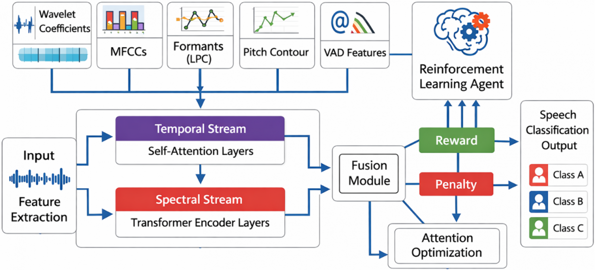
In this work, a novel hybrid architecture is suggested for speech categorization. The features like Wavelet Transform, MFCCs, Linear Predictive Coding (LPC), Formant Frequencies, Pitch Contour, and Voice Activity Detection (VAD) are extracted from the input signal to comprehensively learn the speech signal. Then, the dual stream transformer is used to model the complex nature of speech. Also, RL is applied to optimize the attention weights in the network. The proposed model is capable of improving its performance iteratively and well adapts to the intricacies of speech signals. The overall workflow is given in Figure 1.
Figure 1. Workflow of the proposed classification system
3.1 Feature extraction
Feature extraction involves converting the raw input data into a set of useful features. It captures relevant information and eliminates irrelevant features. The model combines Wavelet Transform, MFCCs, Formant Frequencies, Pitch Contour, and VAD features to represent speech signals comprehensively.
3.2 Wavelet transform features
Wavelet transforms provide a time-frequency decomposition of a signal. In wavelet analysis, the signal is decomposed into different frequency bands using various wavelet functions. Given an input signal x(t), the wavelet transform at scale a and translation b is defined as (Eq. (1)):
$W(a, b)=\int_{-\infty}^{\infty} x(t) \psi\left(\frac{t-b}{a}\right) d t$ (1)
where, $\psi$ is the mother wavelet function, a controls the scale (dilation) of the wavelet, b shifts the wavelet along the time axis. In discrete form, this becomes (Eq. (2)):
$W[a, b]=\sum_{n=0}^{N-1} x_n \psi\left(\frac{n-b}{a}\right)$ (2)
This decomposition provides a set of wavelet coefficients. This coefficient represents the signal's characteristics at different scales and locations in time. After decomposition, the features can be extracted from the resulting wavelet coefficients $\left\{c_1, c_2, \ldots, c_k\right\}$. These features are as follows (Eq. (3) to Eq. (6)) :
Mean:
$\mu=\frac{1}{N} \sum_{i=1}^N c_i$ (3)
The mean represents the average value of the wavelet coefficients. It gives a measure of the overall signal magnitude at a given decomposition level.
Standard Deviation:
$\sigma=\sqrt{\frac{1}{N} \sum_{i=1}^N\left(c_i-\mu\right)^2}$ (4)
The standard deviation measures how much the coefficients vary from the mean. It captures the spread or variability of the signal at that level.
Maximum and Minimum:
$\max (c)=\max \left(c_1, c_2, \ldots, c_k\right), \min (c)=\min \left(c_1, c_2, \ldots, c_k\right)$ (5)
The maximum and minimum values capture the largest and smallest amplitudes in the signal. These help identify peaks or extreme variations in the signal.
Energy:
$ E=\sum_{i=1}^N c_i^2$ (6)
Energy measures the total power of the signal at a particular scale. It is used to quantify the signal’s strength and activity over time.
3.3 Mel-Frequency Cepstral Coefficient
MFCCs are widely used in speech processing to represent the short-term power spectrum of a sound. The process of calculating MFCCs involves several steps. Initially, the Fourier transform is applied to convert the signal into the frequency domain. Then, the Mel-Scale Filter Bank is applied to apply a series of filters which mimic the human ear's perception of pitch. After that, logarithmic compression is used to simulate the loudness perception of the human auditory system. Finally, the Discrete Cosine Transform (DCT) is used to reduce the dimensionality of the features. Given an audio signal x(t), MFCCs are derived as follows:
Mel-Frequency Cepstral Coefficient computation
Short-Time Fourier Transform (STFT): Divide the input into short overlying segments and compute the Fourier Transform for each part as follows (Eq. (7)):
$ X(t, f)=\int_{-\infty}^{\infty} x(\tau) e^{-j 2 \pi f \tau} d \tau$ (7)
where, x(τ) is the input signal as a function of time τ, X(t, f) is the Fourier transform of the short-time segment centered at time t and frequency f, j is the imaginary unit. This computes the frequency content over short overlapping windows of the signal.
Mel-Scale Filtering: Convert the frequency axis to the Mel scale, which is a logarithmic scale more closely related to human hearing. The Mel scale is defined as (Eq. (8)):
$ M(f)=2595 \log _{10}\left(1+\frac{f}{700}\right)$ (8)
where, $f$ is the frequency in $\mathrm{Hz}$, $M(f)$ is the Mel-scaled frequency. This converts linear frequency to a logarithmic scale mimicking human hearing.
DCT for MFCCs: After filtering, the log-magnitude spectrogram is transformed using the DCT (Eq. (9)):
$ \mathrm{MFCC}_n=\sum_{k=0}^{K-1} \log \left|S_k\right| \cdot \cos \left(\frac{n \pi(2 k+1)}{2 K}\right)$ (9)
where, $S_k$ are the log-magnitude coefficients, $K$ is the number of Mel-filter bins, $n$ is the index of the MFCC. DCT compresses the spectral information into a smaller number of coefficients.
3.4 Linear Predictive Coding features
LPC is used to model the signal as a linear combination of previous samples. It assumes that each sample is a linear function of its past values plus some noise. For a signal x(t), LPC estimates the current sample based on previous samples. The equation is (Eq. (10)):
$ x(t)=\sum_{k=1}^p a_k x(t-k)+e(t)$ (10)
where, $a_k$ are the LPC coefficients, $p$ is the order of the LPC model, $e(t)$ is the residual error. The formants of the signal which represent resonant frequencies in the human vocal tract. It can be extracted by solving the Toeplitz matrix using the autocorrelation method (Eq. (11)):
$ R=\operatorname{Autocorr}(x(t)) \Rightarrow a=\operatorname{SolveToeplitz}(R)$ (11)
where, Autocorr$(x(t))$ is the autocorrelation of the signal. It is used to estimate LPC coefficients. SolveToeplitz$(R)$ is the algorithm to solve the Toeplitz system formed by $R$ to get $a_k$ (LPC coefficients). Then, the Formant frequencies can be computed by analyzing the roots of the LPC polynomial.
3.5 Pitch contour features
The pitch of an audio signal represents the perceived fundamental frequency. Pitch tracking involves extracting the frequency of the fundamental tone in a signal. Pitch $f_0$ is determined by analyzing the periodicity of the signal and it can be computed using autocorrelation. Given an audio signal $x(t)$, the pitch $f_0$ is detected by (Eq. (12)):
$ \operatorname{ACF}(\tau)=\sum_{t=0}^{T-\tau} x(t) x(t+\tau)$ (12)
where, τ is the time shift, and the peak of the autocorrelation function corresponds to the fundamental period.
3.6 Voice Activity Detection
VAD is the process of identifying whether a segment of speech contains actual speech or silence. VAD can be performed by analyzing energy and zero-crossing rate. The energy measures the strength of the signal in a frame (Eq. (13)):
$E=\sum_{t=0}^{T-1} x(t)^2$ (13)
where, $x(t)$ is the input audio signal at time $t$, $T$ is the total number of samples in the frame.
Zero-Crossing Rate (ZCR): Measures the number of times the signal crosses the zero-axis (Eq. (14)):
$Z C R=\frac{1}{T} \sum_{t=1}^{T-1} \mathbb{I}(x(t) \cdot x(t-1)<0)$ (14)
where, $\mathbb{I}$ is an indicator function, $x(t) \cdot x(t-1)<0$ checks if the signal crosses the zero axis between consecutive samples.
3.7 Spectral features
Spectral features capture the frequency content of an audio signal. It is used to understand the tonal characteristics. The spectral centroid measures the "center of mass" of the spectrum, which gives an idea of the brightness of a sound. It is computed as in Eq. (15):
$\text { Centroid }=\frac{\sum_f f \cdot S(f)}{\sum_f S(f)}$ (15)
where, S(f) is the spectral magnitude at frequency f.
The spectral rolloff represents the frequency below which a specified percentage of the total spectral energy lies (Eq. (16)):
$\operatorname{Rolloff}=\min \left(f: \sum_{f=0}^{f_{\text {max }}} S(f)>\alpha \sum_{f=0}^{f_{\text {max }}} S(f)\right)$ (16)
where, $f_{\max }$ is the maximum frequency in the frame and $\alpha$ is typically set to $85 \%$ to capture the spectral shape.
3.8 Dual-Stream Transformer
In this work, a Dual-Stream Transformer-based signal processing model is proposed. The main aim of the model is to extract both temporal and spectral features of data. It uses two parallel transformer encoders: one for temporal dependencies and another for spectral dependencies. Then, the outputs are combined through a cross-attention mechanism to refine the learning process. To further optimize the attention mechanism, RL is used to dynamically adjust attention weights based on the model's performance.
The input to the model is a sequence of data, which is first projected into a higher-dimensional space using a linear transformation. This step is used to convert the input data to a more suitable space for the transformer model to process, as follows (Eq. (17)):
$x_{\text {proj }}=W_{\text {proj }} x+b_{\text {proj }}$ (17)
where, $x$ is the input sequence, $W_{\text {proj}}$ is the projection matrix, $b_{\text {proj}}$ is the bias vector. Then, the projected input is passed to the temporal and spectral streams.
3.9 Temporal Stream Encoder
The Temporal Stream processes the input data considering the sequential, time-based dependencies in the data. The Transformer Encoder is used for this, where each encoder layer is defined as (Eq. (18)):
$\operatorname{Attention}(Q, K, V)=\operatorname{Softmax}\left(\frac{Q K^T}{\sqrt{d_k}}\right) V$ (18)
where, Q = Query, K = Key, V = Value, dk = Dimension of the key vector. The output of each encoder layer is passed to the next layer. The final temporal features are obtained as follows (Eq. (19)).
$h_{\text {temp}}=\text {TransformerEncoder}\left(x_{\text {proj}}\right)$ (19)
Spectral Stream Encoder
Similarly, the Spectral Stream focuses on the frequency-based dependencies. It uses another Transformer Encoder to learn features specific to the frequency domain. The process is similar to the temporal stream (Eq. (20)):
$h_{\text {spec}}=\text {TransformerEncoder}\left(x_{\text {proj}}\right)$ (20)
Cross-Attention Mechanism
The model combines the outputs using a cross-attention mechanism. This is where the attention weights between the two streams are learned (Eq. (21)):
$\operatorname{Cross-Attention}(T, S)=\operatorname{MultiHeadAttention}(T, S, S)$ (21)
where, T = Temporal features from the temporal stream, S = Spectral features from the spectral stream. The cross-attention mechanism computes attention between these two feature sets. It is mainly used for the model to align the most relevant temporal and spectral components.
3.10 Attention optimization via Reinforcement Learning
In conventional Transformer models, attention mechanisms are used to focus on the most relevant parts of the input sequence during the encoding process. The core idea is that the model assigns weights to different parts of the sequence. This process is mainly used to focus on the most important features. However, the allocation of attention across different parts of the sequence is often fixed during training. In this work, RL is used to dynamically adjust these attention weights based on the model's execution. The goal is to optimize the attention weights to improve the model's learning.
3.11 Reinforcement Learning setup for attention optimization
The RL Agent is responsible for adjusting the attention weights during training. This process involves learning policies that define how attention should be distributed across the sequence. The RL agent performs the following steps:
3.12 Policy network
The policy network learns to output a probability distribution over actions based on the state of the model. The output of the policy network is a set of probabilities $\pi_\theta(a \mid s)$, where $\theta$ are the parameters of the policy network, $a$ is the action (which attention head to enhance), and sis the state (the hidden features of the transformer). The policy network is typically implemented as a fully connected neural network and is trained using policy gradient methods.
3.13 Value network
The value network provides an estimate of the value V(s) of a given state. The value network outputs a scalar that represents how good the current state is in terms of expected future rewards. The advantage is computed as (Eq. (22)):
$A\left(s_t, a_t\right)=R_t-V\left(s_t\right)$ (22)
where, $A\left(s_t, a_t\right)$ is the advantage at time step $t, R_t$ is the return (cumulative future rewards), $V\left(s_t\right)$ is the value of the state at time $t$.
Action: Scaling Attention Weights
The RL agent's action corresponds to scaling specific attention heads. In a typical multi-head attention mechanism, the attention matrix is calculated as (Eq. (23)):
$\operatorname{Attention}(Q, K, V)=\operatorname{Softmax}\left(\frac{Q K^T}{\sqrt{d_k}}\right) V$ (23)
where, $Q, K$, and $V$ are the Query, Key, and Value matrices, respectively, $d_k$ is the dimension of the key vectors. Each head in multi-head attention learns a different transformation of the input sequence. It is used for the system to concentrate on various parts of the sequence. The RL agent selects a specific attention head $i$ and scales its attention weights by a factor $\lambda$ (Eq. (24)):
$\hat{A}_i=A_i \cdot \lambda$ (24)
where, $A_i$ is the attention matrix for head $i$, $\lambda$ is the scaling factor. The goal is for the RL agent to learn to amplify the most relevant attention heads and reduce the concentration on irrelevant ones.
RL Objective: Policy Loss
The RL agent is trained to maximize cumulative rewards over time. The loss function for training the policy network is based on the REINFORCE algorithm, which aims to maximize the expected return (Eq. (25)):
$L_{\mathrm{policy}}=-\mathbb{E}\left[r_t \cdot \log \left(\pi_\theta(a \mid s)\right)\right]$ (25)
where, $r_t$ is the reward at time $t$ (e.g., classification accuracy), $\pi_\theta(a \mid s)$ is the probability of selecting action $a$ in state saccording to the policy network. This loss encourages the model to select attention heads that lead to high rewards.
Value Loss
The value network is used to estimate how good the current state is. The value loss is computed as the mean squared error between the predicted value $V(s)$ and the actual return $R_t$ (Eq. (26)):
$L_{\text {value }}=\mathbb{E}\left[\left(V\left(s_t\right)-R_t\right)^2\right]$ (26)
where, $V\left(s_t\right)$ is the predicted value for the state $s_t, R_t$ is the return, i.e., the sum of rewards from time step $t$. This loss is used for the value network to provide better value estimates' Entropy Regularization.
To ensure the RL agent explores different actions and does not get stuck in suboptimal solutions, an entropy regularization term is added. This supports the policy network to maintain diversity in its action selections. The entropy of the policy distribution $H(\pi)$ is computed as (Eq. (27)):
$H(\pi)=-\sum_a \pi_\theta(a \mid s) \log \left(\pi_\theta(a \mid s)\right)$ (27)
The total RL loss combines the policy loss, value loss, and the entropy term (Eq. (28)):
$L_{\mathrm{RL}}=L_{\mathrm{policy}}+\frac{1}{2} L_{\mathrm{value}}-\beta \cdot H(\pi)$ (28)
where, $\beta$ is the entropy coefficient that controls the importance of the entropy term. The total loss during training relates to the classification loss and the RL loss. The classification loss is computed as the cross-entropy loss between the predicted and true labels. The RL loss encourages the model to adjust its attention mechanism based on rewards as follows (Eq. (29)).
$L_{\text {total }}=L_{\text {classification }}+\lambda_{\mathrm{RL}} L_{\mathrm{RL}}$ (29)
where, $L_{\text {classification }}$ is the classification loss, $\lambda_{\mathrm{RL}}$ is a scaling factor that controls the importance of the RL loss in the total loss function. The overall Pseudocode is given below:
Pseudocode
Initialize attention weights W_att randomly
for epoch = 1 to MaxEpochs:
for batch in training_data:
T, S = TemporalStream(batch), SpectralStream(batch)
H = CrossAttention(T, S, W_att)
pred = Classifier(H)
reward = Accuracy(pred, true_labels)
W_att = W_att + learning_rate * $\nabla$_W_att(reward)
if reward converges:
break
In the proposed Dual-Stream Transformer, standard backpropagation is improved with RL to fine-tune attention weights and improve classification performance. Initially, attention weights $W_{\text {att }}$ are randomly initialized. For each training batch, temporal and spectral features are extracted and combined via cross-attention. The resulting representation is passed to the classifier. The reward is computed based on the classification accuracy or F1-score. Then, RL updates the attention weights in the direction that maximizes this reward. This process repeats over epochs until convergence.
Here, the state represents the combined temporal and spectral features. The action adjusts attention weights based on the reward. Reward defines the batch classification accuracy. It updates based on the equation of $W_{\text {att }}^{(t+1)}=W_{\text {att }}^{(t)}+ \alpha \nabla_{W_{\text {att }}} R_t$ with learning rate $\alpha=0.01$. The training stability is achieved by reward smoothing and gradient clipping with a convergence criterion of $\Delta$ Reward $< \, 0.001$ for 5 consecutive epochs.
3.14 Feature fusion and classification
After weight optimization, the temporal and cross-attended features are fused together. The fusion step concatenates the features from both streams (Eq. (30)):
$h_{\text {fused}}=\operatorname{Concat}\left(h_{\text {temp}}, h_{\text {cross}}\right)$ (30)
The fused features are passed through a fusion layer of a fully connected layer to reduce dimensionality and learn more complex representations as follows (Eq. (31)):
$h_{\text {fused }}=W_{\text {fusion }} \cdot h_{\text {fused }}+b_{\text {fusion }}$ (31)
where, $W_{\text {fusion}}$ is the fusion weight matrix, $b_{\text {fusion}}$ is the bias vector.
Finally, the classification head is applied to the fused features to make predictions(Eq. (32)):
$y=\operatorname{Softmax}\left(W_{\text {class}} \cdot h_{\text {fused}}+b_{\text {class}}\right)$ (32)
where, $W_{\text {class}}$ is the classification weight matrix, $b_{\text {class}}$ is the classification bias, $y$ is the predicted class.
The proposed dual stream transformer model is coded in Python and implemented in the Google Colab environment. The accuracy of the model is assessed using the RAVDESS dataset. This dataset consists of high-quality emotional speech recordings from 24 professional actors expressing eight distinct emotions. The Dual-Stream Transformer model uses 4 layers for both the temporal and spectral transformer encoders. In each layer, 8 attention heads are used with the model dimension of 256. The cross-attention module uses 8-head multi-head attention. In RL, the optimization uses a learning rate of 0.01 and a convergence criterion of a change in reward of less than 0.001 for 5 consecutive epochs. The training is performed using the Adam optimizer with β1 = 0.9, β2 = 0.999, and ε = 1 × 10⁻⁸. The batch size is set to 32 with the dropout rate of 0.1 in the transformer layers. The number of epochs is set to 50. The cross-entropy loss function is applied for model optimization.
Initially, the dataset is pre-processed with silence removal and normalisation. To solve the data imbalance and to generate new speech samples, the Generative Adversarial Networks (GANs) model is applied. The GAN model is trained on the training data partition only and no test-set samples are used at any stage of GAN training. The dataset is first split into training, validation, and test sets before any feature extraction. The synthetic samples are generated only from the training distribution and are added exclusively to the training set to avoid data leakage.To validate the quality of the generated dataset, the statistical properties of the samples are compared. The generator creates realistic audio features. The discriminator ensures quality by distinguishing real from generated samples. Then, the augmented data are added to the training set. It improves the distribution uniformity across classes. This balanced dataset is used for the model to learn better representations for minority classes. It reduces bias and improves overall classification accuracy and generalization. Table 2 compares statistical properties of original vs GAN-generated samples for key features. The closeness of values indicates that the GAN maintains the distribution of the original dataset. It generates additional samples to balance underrepresented classes.
Table 2. Statistical comparison of original vs. Generative Adversarial Network (GAN)-generated samples
|
Feature |
Dataset Type |
Mean |
Std Dev |
Min |
Max |
|
MFCC_C1 |
Original |
12.3 |
3.4 |
5.1 |
19.8 |
|
MFCC_C1 |
GAN-Generated |
12.5 |
3.5 |
5.0 |
20.1 |
|
MFCC_C2 |
Original |
10.8 |
2.9 |
4.2 |
17.6 |
|
MFCC_C2 |
GAN-Generated |
11.0 |
3.0 |
4.3 |
17.8 |
|
Pitch (Hz) |
Original |
210.5 |
45.2 |
110.0 |
310.0 |
|
Pitch (Hz) |
GAN-Generated |
212.0 |
46.0 |
112.0 |
312.0 |
|
Energy |
Original |
0.75 |
0.20 |
0.35 |
1.20 |
|
Energy |
GAN-Generated |
0.76 |
0.21 |
0.36 |
1.22 |
|
Formant F1 (Hz) |
Original |
550.0 |
120.0 |
300.0 |
780.0 |
|
Formant F1 (Hz) |
GAN-Generated |
552.0 |
118.0 |
305.0 |
782.0 |
The following standard classification metrics are used for evaluation:
Accuracy (Acc): The proportion of correctly classified samples out of all samples. It can be computed as follows (Eq. (33)):
$\mathrm{Acc}=\frac{\mathrm{TP}+\mathrm{TN}}{\mathrm{TP}+\mathrm{TN}+\mathrm{FP}+\mathrm{FN}}$ (33)
Precision (Precision): The proportion of true positive predictions (correctly predicted emotions) among all positive predictions. It can be computed as follows (Eq. (34)):
$\text { Precision }=\frac{\mathrm{TP}}{\mathrm{TP}+\mathrm{FP}}$ (34)
Recall (Recall): The proportion of actual positive samples (true instances of the emotion) that were correctly identified by the model. It can be computed as follows (Eq. (35)):
$\text { Recall }=\frac{\mathrm{TP}}{\mathrm{TP}+\mathrm{FN}}$ (35)
F1-Score (F1): The harmonic mean of precision and recall, providing a single metric that balances both. It can be computed as follows (Eq. (36)):
$\mathrm{F} 1=2 \cdot \frac{\text { Precision } \cdot \text { Recall }}{\text { Precision }+ \text { Recall }}$ (36)
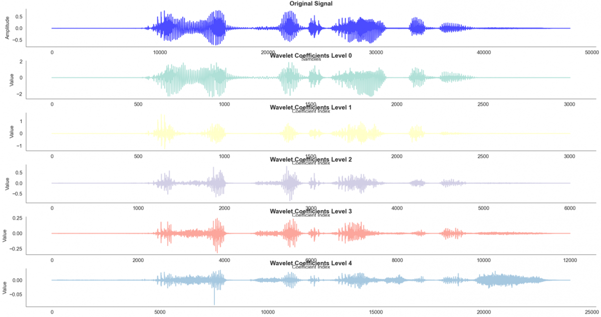
Figure 2 shows an original signal with its decomposition using a wavelet transform. The topmost plot represents the original signal in blue. Each successive waveform corresponds to the wavelet coefficients at different decomposition levels (from Level 0 to Level 4). These levels represent progressively finer resolutions of the signal. Each subsequent plot shows higher-frequency details captured at the corresponding wavelet decomposition level.
Figure 2. Input signal with its wavelets
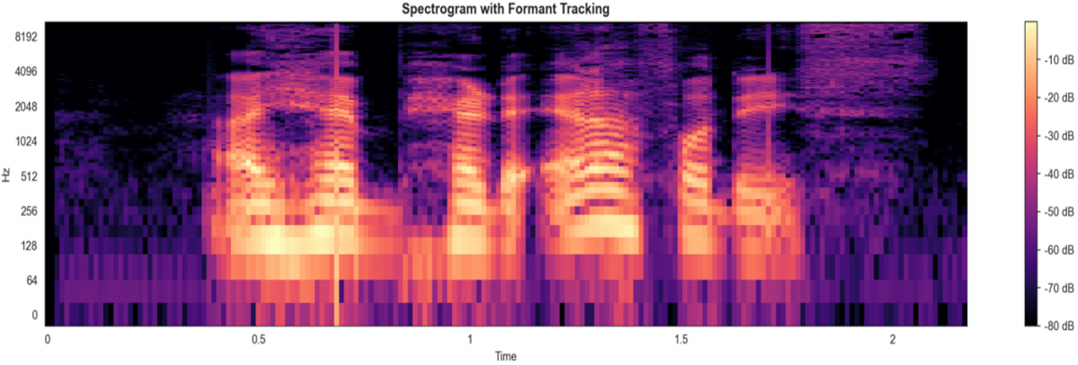
Figure 3 shows the spectrogram of the signal. The color intensity represents the amplitude of frequencies across time. The spectrogram is overlaid with formant tracking which tracks the key resonant frequencies (formants) in speech. These formants are important for vowel sounds which are visualised by distinct features across time.
Figure 3. Spectrogram of the input signal (X-axis: time (seconds), Y-axis: frequency (Hz))
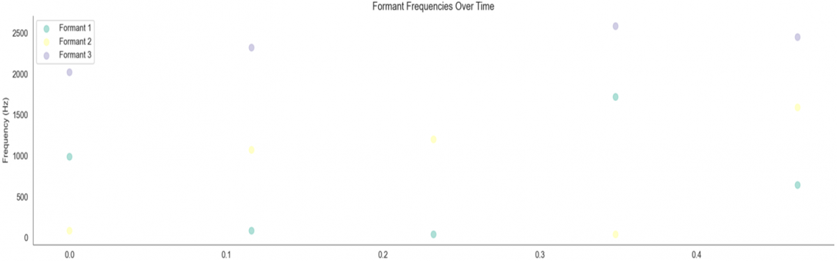
Figure 4 shows the frequencies of the first three formants over time. Each point represents the frequency at a specific time segment. The plot uses varying colours to represent the different formants.
Figure 4. Formant frequencies over time (X-axis: time (seconds), Y-axis: frequency (Hz))
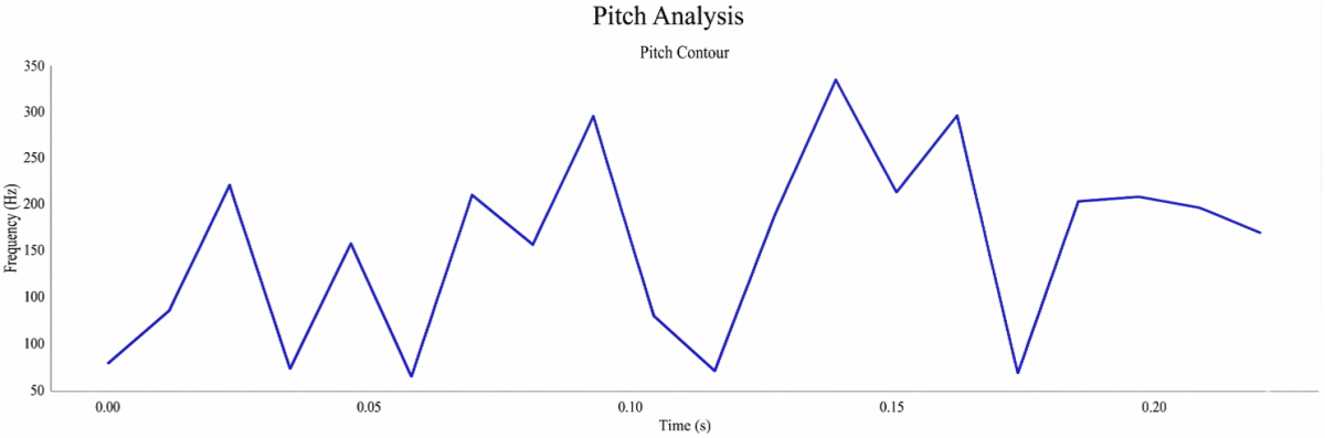
Figure 5 presents a pitch contour graph of signal processing. This plot tracks the variation in pitch of the signal over time. The pitch contour is represented by a blue line. It shows the periodicity and fluctuations of the speaker’s pitch. This is the main feature to detect speech intonation and prosody.
Figure 5. Pitch analysis (X-axis: time (seconds), Y-axis: pitch frequency (Hz))
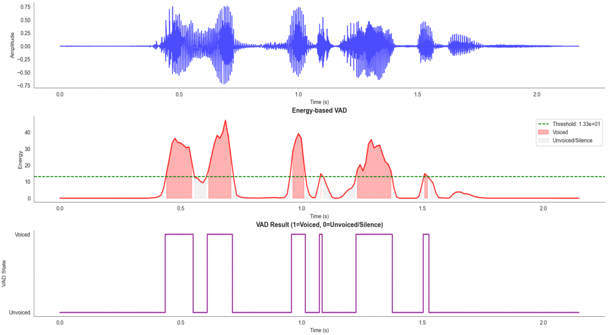
Figure 6 shows the VAD plot of the signal. This plot tracks the energy of the signal and indicates voiced and unvoiced speech segments. The threshold is marked by a dashed green line with regions above the threshold highlighted in red as voiced speech and below as unvoiced or silence. It marks segments of voiced and unvoiced speech using a purple bar. This result is critical for classification that needs to distinguish between speech and non-speech parts of an audio signal.
Figure 6. Energy-based Voice Activity Detection
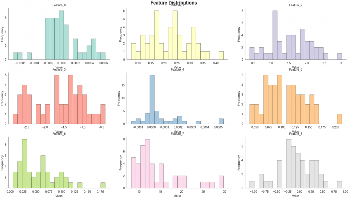
Figure 7 shows the histogram of different features in the dataset. Each histogram represents the frequency distribution of a particular feature. These features seem to span a range of values with each distribution presenting its own shape and spread. This distribution is used to understand the characteristics of each feature.
Figure 7. Feature distributions (X-axis: feature value, Y-axis: frequency count)
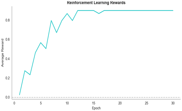
Figure 8 shows the average reward over epochs in an RL training process. As the training progresses, the reward steadily increases. It is observed that the model is learning and improving its performance over time. The line starts with a lower reward and gradually rises over epochs.
Figure 8. Reinforcement Learning (RL) rewards
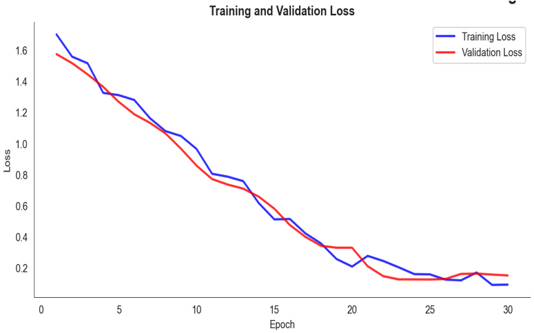
Figure 9 shows the change in training and validation loss across epochs. The blue line represents the training loss, and the red line represents the validation loss. Both lines decrease steadily over time which indicates that the model is improving with training. The loss values are close to each other toward the end which suggests that the model is generalizing well and there's no significant overfitting or underfitting.
Figure 9. Model training and validation loss
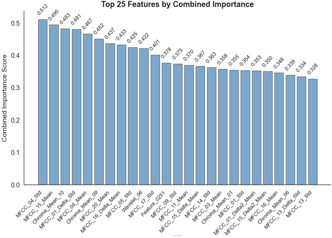
Figure 10 shows the top 25 features by their combined importance score. The features like MFCC_C4_Std and MFCC_C1_Mean are measured based on their ability to contribute to the model's decision-making process. The higher scores indicate more important features in the context of the analysis.
Figure 10. Feature importance plot (X-axis: feature names, Y-axis: importance score)
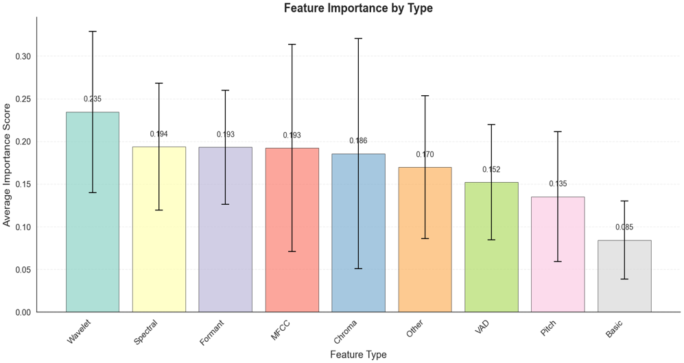
Figure 11 shows the average importance score for different types of features like Wavelet, Spectral, MFCC, and others. The feature types with higher average importance scores like Wavelet and Chroma are considered more relevant to the task at hand, whereas the basic features have the lowest importance.
Figure 11. Feature importance by type
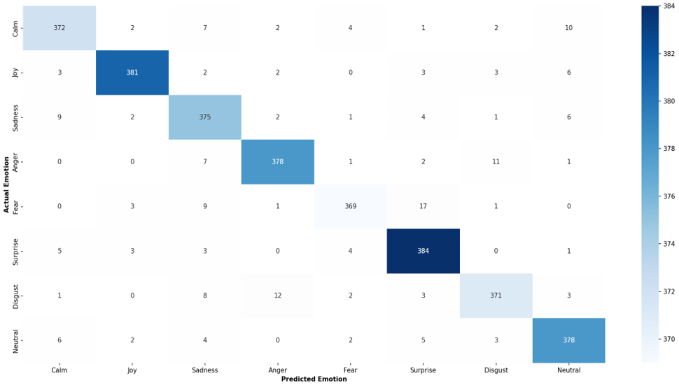
Figure 12 represents a confusion matrix of predicted versus actual emotions in a classification task. The color intensity indicates the number of samples predicted for each emotion. In the diagonal, the highest values confirm that the model is highly efficient at recognising complex emotional states. Table 3 summarises the model's performance in classifying emotions. Overall, the model performs well across all emotions. For Joy, the model has the highest precision (96.9%) and recall (95.3%) with a strong F1-score (96.1%). The model shows slightly lower recall for the Sadness and Fear classes.
Figure 12. Confusion matrix plot
Table 3. Performance of the model for different classes
|
Emotion |
Precision |
Recall |
F1-Score |
|
Calm |
0.939 |
0.930 |
0.935 |
|
Joy |
0.969 |
0.953 |
0.961 |
|
Sadness |
0.904 |
0.938 |
0.920 |
|
Anger |
0.957 |
0.945 |
0.951 |
|
Fear |
0.964 |
0.923 |
0.943 |
|
Surprise |
0.923 |
0.960 |
0.941 |
|
Disgust |
0.942 |
0.928 |
0.935 |
|
Neutral |
0.933 |
0.945 |
0.939 |
The performance of the model with existing models is given in Table 4. The Proposed model achieves the highest accuracy of 94.2. The 2D-CNN + XGBoost shows an accuracy of 93.1%, and the Hybrid CNN + SNN shows an accuracy performance at 93%. The CNN-LSTM and DNN models show accuracies of 92.8% and 92.5%, respectively. The Fisher rate + SVM method shows a relatively lower accuracy compared to the other models.
Table 4. Performance comparison of the model
|
Method |
Accuracy |
|
Fisher rate + SVM |
89.2 |
|
EMD |
87 |
|
MFCC + Modulation spectral features + CNN |
90 |
|
Autoencoder+ SVM |
88.6 |
|
VMD + SVM |
85 |
|
MCJD + PCA + Genetic Algorithm |
91 |
|
CNN-LSTM |
92.8 |
|
DNN |
92.5 |
|
2D-CNN + XGBoost |
93.1 |
|
MRHT + CNN |
92.4 |
|
Hybrid CNN + SNN |
93 |
|
Proposed |
94.2 |
To further validate the performance, the model is evaluated on three different datasets, like TED‑LIUM, CSS10, and LibriSpeech ASR Corpus. The description of the dataset is given in Table 5.
Table 5. Dataset description
|
Dataset |
# Samples |
# Speakers |
Male/Female Ratio |
# Emotions / Classes |
Duration (hrs) |
|
RAVDESS |
1,440 |
24 |
12/12 |
8 |
1.5 |
|
TED-LIUM |
2,351 |
118 |
72/46 |
10 |
20 |
|
CSS10 |
10,000 |
10 |
5/5 |
8 |
12 |
|
LibriSpeech ASR |
100,000 |
2484 |
1250/1234 |
10 |
281 |
These datasets are designed for automatic speech recognition and do not contain emotion labels. Therefore, in this study, we redefine the task as a speech representation-based classification problem. The class labels are generated using feature-driven clustering over MFCC, pitch, formant, and spectral embeddings. This step is used to evaluate the model under a cross-domain speech categorization setting rather than emotion recognition.The obtained results are given in Table 6. On TED‑LIUM, the model maintained strong performance with an accuracy of 90.5%. Likewise, on the CSS10 data set, the model achieves an accuracy of 91.2%. It proves that the model generalizes well to expressive speech from multiple speakers and languages. On the LibriSpeech ASR dataset, the model achieved an accuracy of 89.8%. For all datasets, precision, recall, and F1‑scores remain consistently high.
Table 6. Performance comparison with other datasets
|
Dataset |
Accuracy (%) |
Precision |
Recall |
F1‑Score |
|
RAVDESS |
94.2 |
0.945 |
0.943 |
0.944 |
|
TED‑LIUM |
90.5 |
0.91 |
0.90 |
0.905 |
|
CSS10 |
91.2 |
0.92 |
0.91 |
0.915 |
|
LibriSpeech ASR |
89.8 |
0.90 |
0.89 |
0.895 |
An ablation study was performed on the RAVDESS dataset to analyze the contribution of each component in the proposed model. The model is tested under different configurations. The results are given in Table 7.
Table 7. Ablation study of each component
|
Configuration |
Accuracy (%) |
Precision |
Recall |
F1-Score |
|
Temporal-Only Transformer |
91.5 |
0.918 |
0.915 |
0.916 |
|
Spectral-Only Transformer |
90.8 |
0.912 |
0.908 |
0.910 |
|
Dual-Stream Transformer (No RL) |
93.5 |
0.938 |
0.935 |
0.936 |
|
Dual-Stream Transformer + RL |
94.2 |
0.945 |
0.943 |
0.944 |
The model using a single stream limits performance with an accuracy below 92%. The model including both streams without RL, increases accuracy to 93.5%. It indicated that combining temporal and spectral features provides richer representations. The full model with RL-based attention optimization achieves the highest performance.
Likewise, the feature-wise ablation study is carried out to analyze feature importance. The results are summarised in Table 8. The ablation results indicate that Wavelet and MFCC features contribute the most to classification performance. The model with multiple speech features enhances model generalization and robust emotion recognition.
Table 8. Feature importance analysis
|
Feature Set Removed |
Accuracy (%) |
Precision |
Recall |
F1-Score |
|
None (All Features) |
94.2 |
0.945 |
0.943 |
0.944 |
|
Wavelet |
91.5 |
0.918 |
0.915 |
0.916 |
|
MFCC |
92.0 |
0.922 |
0.920 |
0.921 |
|
Pitch |
93.1 |
0.932 |
0.930 |
0.931 |
|
Formant |
93.5 |
0.936 |
0.933 |
0.934 |
|
VAD |
93.8 |
0.940 |
0.938 |
0.939 |
To assess the reliability of the proposed dual-stream transformer model, a 5-fold cross-validation is performed on the RAVDESS dataset. The results are summarised in Table 9. The standard deviation indicates the variability of each metric across the folds. The 95% confidence interval provides a statistical range within which the true performance metric is expected to lie with 95% confidence.
Table 9. Cross-validation analysis
|
Metric |
Mean Value |
Std Dev |
95% Confidence Interval |
|
Accuracy (%) |
94.2 |
0.8 |
[93.1, 95.3] |
|
Precision |
0.945 |
0.007 |
[0.931, 0.957] |
|
Recall |
0.943 |
0.009 |
[0.926, 0.955] |
|
F1-Score |
0.944 |
0.008 |
[0.929, 0.956] |
The results show low standard deviation across folds. It proves the stable performance of the model. The narrow confidence intervals confirm that the model consistently achieves high classification metrics and can generalize well across different subsets of data.
To analyses the cross-language performance, the model is tested for the CSS10 dataset with different languages. It includes English, Spanish, German, Japanese, and French language speeches as given in Table 10. This evaluation is used to determine whether the model’s feature extraction and classification capabilities are robust across linguistic variations.
Table 10. Classification performance metrics for cross-language
|
Language |
Accuracy (%) |
Precision |
Recall |
F1-Score |
|
English |
91.2 |
0.918 |
0.915 |
0.916 |
|
Spanish |
90.8 |
0.912 |
0.908 |
0.910 |
|
German |
90.5 |
0.909 |
0.905 |
0.907 |
|
Japanese |
91.0 |
0.914 |
0.910 |
0.912 |
|
French |
90.7 |
0.911 |
0.907 |
0.909 |
The results show that the model maintains consistently high performance across different languages. The accuracy varies from 90.5% to 91.2%.
In this work, a threefold hybrid approach is proposed for speech signal classification. This model accurately models the complex and non-stationary nature of speech signals. By integrating different features, the model captures both the temporal nature and the spectral behaviour of speech in a complete manner. The dual-stream transformer network, combined with RL, improves the model’s capability to handle different and intricate speech patterns. This work contributes to the ongoing evolution of intelligent speech classification technologies and offers a foundation for further innovations in the integration of AI models. The current model is primarily evaluated on clean speech datasets. The performance may degrade in real-world noisy conditions. Future work will focus on lightweight model design with noise-robust features.
[1] Grozdić, T., Jovičić, S.T. (2017). Whispered speech recognition using deep de-noising autoencoder and inverse filtering. IEEE/ACM Transactions on Audio, Speech, and Language Processing, 25(12): 2313-2322. https://doi.org/10.1109/TASLP.2017.2738559
[2] Joysingh, S.J., Vijayalakshmi, P., Nagarajan, T. (2023). Quartered spectral envelope and 1D-CNN-based classification of normally phonated and whispered speech. Circuits, Systems, and Signal Processing, 42: 3038-3053. https://doi.org/10.1007/s00034-022-02263-5
[3] Abdusalomov, A.B., Safarov, F., Rakhimov, M., Turaev, B., Whangbo, T.K. (2022). Improved feature parameter extraction from speech signals using machine learning algorithm. Sensors, 22(21): 8122. https://doi.org/10.3390/s22218122
[4] Jiang, N., Liu, T. (2020). An improved speech segmentation and clustering algorithm based on SOM and k-means. Mathematical Problems in Engineering, 2020(1): 3608286. https://doi.org/10.1155/2020/3608286
[5] Ye, F., Yang, J. (2021). A deep neural network model for speaker identification. Applied Sciences, 11(8): 3603. https://doi.org/10.3390/app11083603
[6] Narmadha, G., Deivasigamani, S., Muthukumar, V., Freitas, L.I., Ahmad, R.B., Sakthivel, B. (2023). Detection of human stress using optimized feature selection and classification in ECG signals. Mathematical Problems in Engineering, 2023: 3356347. https://doi.org/10.1155/2023/3356347
[7] Sun, L., Fu, S., Wang, F. (2019). Decision tree SVM model with Fisher feature selection for speech emotion recognition. EURASIP Journal on Audio, Speech, and Music Processing, 2019: 2. https://doi.org/10.1186/s13636-018-0145-5
[8] Batur Dinler, Ö., Aydin, N. (2020). An optimal feature parameter set based on gated recurrent unit recurrent neural networks for speech segment detection. Applied Sciences, 10(4): 1273. https://doi.org/10.3390/app10041273
[9] Pitsikalis, V., Maragos, P. (2009). Analysis and classification of speech signals by generalized fractal dimension features. Speech Communication, 51(12): 1206-1223. https://doi.org/10.1016/j.specom.2009.06.005
[10] Chen, L., Mao, X., Xue, Y., Cheng, L.L. (2012). Speech emotion recognition: Features and classification models. Digital Signal Processing, 22(6): 1154-1160. https://doi.org/10.1016/j.dsp.2012.05.007
[11] Kaleem, M., Ghoraani, B., Guergachi, A., Krishnan, S. (2013). Pathological speech signal analysis and classification using empirical mode decomposition. Medical & Biological Engineering & Computing, 51: 811-821. https://doi.org/10.1007/s11517-013-1051-8
[12] Christy, A., Vaithyasubramanian, S., Jesudoss, A., Praveena, M.D.A. (2020). Multimodal speech emotion recognition and classification using convolutional neural network techniques. International Journal of Speech Technology, 23: 381-388. https://doi.org/10.1007/s10772-020-09713-y
[13] Aouani, H., Ayed, Y.B. (2020). Speech emotion recognition with deep learning. Procedia Computer Science, 176: 251-260. https://doi.org/10.1016/j.procs.2020.08.027
[14] Krishnan, P.T., Joseph Raj, A.N., Rajangam, V. (2021). Emotion classification from speech signal based on empirical mode decomposition and non-linear features. Complex & Intelligent Systems, 7: 1919-1934. https://doi.org/10.1007/s40747-021-00295-z
[15] Pravin, S.C., Palanivelan, M. (2021). A hybrid deep ensemble for speech disfluency classification. Circuits, Systems, and Signal Processing, 40: 3968-3995. https://doi.org/10.1007/s00034-021-01657-1
[16] Dendukuri, L.S., Hussain, S.J. (2022). Emotional speech analysis and classification using variational mode decomposition. International Journal of Speech Technology, 25(2): 457-469. https://doi.org/10.1007/s10772-022-09970-z
[17] Sun, L., Huang, Y., Li, Q., Li, P. (2022). Multi-classification speech emotion recognition based on two-stage bottleneck features selection and MCJD algorithm. Signal, Image and Video Processing, 16(5): 1253-1261. https://doi.org/10.1007/s11760-021-02076-0
[18] Chaiani, M., Selouani, S.A., Boudraa, M. (2022). Voice disorder classification using speech enhancement and deep learning models. Biocybernetics and Biomedical Engineering, 42(2): 463-480. https://doi.org/10.1016/j.bbe.2022.03.002
[19] Hama Saeed, M. (2023). Improved speech emotion classification using deep neural network. Circuits, Systems, and Signal Processing, 42: 7357-7376. https://doi.org/10.1007/s00034-023-02446-8
[20] Mohan, M., Dhanalakshmi, P., Kumar, R.S. (2023). Speech emotion classification using ensemble models with MFCC. Procedia Computer Science, 218: 1857-1868. https://doi.org/10.1016/j.procs.2023.01.163
[21] Liu, G., Cai, S., Wang, C. (2023). Speech emotion recognition based on emotion perception. EURASIP Journal on Audio, Speech, and Music Processing, 2023: 22. https://doi.org/10.1186/s13636-023-00289-4
[22] Yücesoy, E. (2024). Gender recognition from speech signal using CNN, KNN, SVM and RF. Procedia Computer Science, 235: 2251-2257. https://doi.org/10.1016/j.procs.2024.04.213
[23] Liu, M., Joseph Raj, A.N., Rajangam, V., Ma, K., Zhuang, Z., Zhuang, S. (2024). Multiscale-multichannel feature extraction and classification through one-dimensional convolutional neural network for speech emotion recognition. Speech Communication, 156: 103010. https://doi.org/10.1016/j.specom.2023.103010
[24] Mishra, S.P., Warule, P., Deb, S. (2024). Speech emotion classification using feature-level and classifier-level fusion. Evolving Systems, 15: 541-554. https://doi.org/10.1007/s12530-023-09550-9
[25] Mishra, S.P., Warule, P., Deb, S. (2025). Speech emotion recognition using multi resolution Hilbert transform based spectral and entropy features. Applied Acoustics, 229: 110403. https://doi.org/10.1016/j.apacoust.2024.110403
[26] Du, C., Liu, F., Kang, B., Hou, T. (2025). Speech emotion recognition based on spiking neural network and convolutional neural network. Engineering Applications of Artificial Intelligence, 147: 110314. https://doi.org/10.1016/j.engappai.2025.110314
[27] Shah, U., Alzubaidi, M., Mohsen, F., Alam, T., Househ, M. (2024). Ensemble-based feature engineering mechanism to decode imagined speech from brain signals. Informatics in Medicine Unlocked, 47: 101491. https://doi.org/10.1016/j.imu.2024.101491
[28] Manoswini, M., Sahoo, B., Swetapadma, A. (2025). A novel speech signal feature extraction technique to detect speech impairment in children accurately. Computers in Biology and Medicine, 195: 110681. https://doi.org/10.1016/j.compbiomed.2025.110681
[29] Banerjee, N., Sethi, N., Borah, S. (2025). Deep analysis of MFCC and MEL spectrogram features to recognize and classify stuttered speech. Multimedia Tools and Applications, 84: 43827-43846. https://doi.org/10.1007/s11042-025-20881-4
[30] Narasinga, V., Khan, H.F.F., Motepalli, K., Mahesh, S., Abraham, A.K., Vuppala, A.K. (2026). Speech signal processing based stuttering classification and clinical studies. Circuits, Systems, and Signal Processing, 45(2): 1171-1198. https://doi.org/10.1007/s00034-025-03264-w