Vinodkumar Reddy Surasani | Hemasundara Reddy Lanka | Raghuvaran Reddy Kalluri | Nagaraju Devarakonda | Sarvani Anandarao*
© 2026 The authors. This article is published by IIETA and is licensed under the CC BY 4.0 license (http://creativecommons.org/licenses/by/4.0/).
OPEN ACCESS
Early and reliable identification of Alzheimer’s disease (AD) from Magnetic Resonance Imaging (MRI) remains challenging because disease-related structural changes are often subtle, spatially distributed, and difficult to model with conventional feature extractors. This study proposes an explainable Swin Transformer and Temporal Convolutional Network (Swin-TCN) framework for MRI-based AD classification. The Swin Transformer is used to learn hierarchical spatial representations from preprocessed brain MRI volumes, while the Temporal Convolutional Network models ordered inter-slice dependencies without the computational burden of recurrent architectures. A Hybrid Attention Mechanism (HAM) further recalibrates channel-level and slice-level information, allowing the model to focus on diagnostically relevant patterns. Differential Evolution (DE) is adopted to optimize key hyperparameters, including the learning rate, batch size, kernel size, dilation rate, and regularization settings. The framework was evaluated on the publicly available Kaggle MRI and Alzheimer’s dataset using subject-wise five-fold cross-validation to reduce the risk of slice-level data leakage. Under the same preprocessing pipeline and data splits, the proposed model outperformed CNN-, recurrent-, and transformer-based baselines, achieving 99.50% accuracy and an area under the curve (AUC) of 0.92. Grad-CAM++ and Integrated Gradients were used to visualize brain regions contributing to the model predictions. These results suggest that the proposed framework provides a high-performing and interpretable approach for MRI-based AD classification, although further validation on external clinical datasets is required before clinical deployment.
Alzheimer’s disease, Magnetic Resonance Imaging, Swin Transformer and Temporal Convolutional Network, Differential Evolution, explainable artificial intelligence, medical image classification
A chronic neurological disease, Alzheimer's disease (AD) progressively deteriorates memory, cognitive function, and day‑to‑day functioning [1]. By 2050, there will be 135.46 million AD cases, according to the World Alzheimer Report, underscoring the critical need for prompt and precise detection [2]. Magnetic Resonance Imaging (MRI) is an essential diagnostic tool, but because AD‑related brain alterations are complicated, manually interpreting MRI results is still difficult [3]. The classification of AD has been investigated using conventional machine learning techniques like Support Vector Machines (SVM) and Random Forest; however, these models depend on manually extracted features and frequently have poor generalization and overfitting [4]. Recurrent models such as Long Short‑Term Memory (LSTM) networks and deep learning approaches, especially Convolutional Neural Networks (CNNs), have increased classification accuracy by automatically learning characteristics from MRI images [5]. However, CNNs by themselves might not be able to identify long‑range connections in images, while LSTMs have problems with vanishing gradients and excessive processing costs [6].
Recent developments in deep learning architectures, such as Vision Transformers (ViTs), have used self‑attention methods to show greater performance in image‑based tasks [7]. But in order to train well, Vision Transformer (ViT) needs a lot of computing power and big datasets, which makes it less useful for medical applications [8]. In order to get beyond these restrictions, this study suggests a brand‑new deep learning framework for AD classification that combines Swin Transformer and Temporal Convolutional Network (Swin-TCN). By using hierarchical self‑attention with shifting windows, the Swin Transformer effectively captures spatial characteristics while preserving high performance and minimizing computational complexity [9]. In the meantime, TCN successfully simulates MRI scan sequence dependencies without the limitations of recurrent structures [10].
Differential Evolution (DE) is also used in this work for hyperparameter optimization, which increases training effectiveness and avoids local minima convergence [11]. DE ensures resilient parameter adjustment by preserving population variety, in contrast to conventional optimization strategies [11]. Furthermore, the system incorporates Explainable AI (XAI) techniques like Grad‑CAM++ and Integrated Gradients to improve model interpretability and enable physicians to see the main brain areas affecting categorization results [12]. The MRI and Alzheimer's dataset, a popular standard for AD research, is utilized to assess the suggested model [3]. According to experimental data, the Swin-TCN model outperforms the earlier CNN‑LSTM and ViT‑BiGRU methods with an accuracy of 99.50%, providing a computationally effective and comprehensible solution for the categorization of AD [13].
The development of an optimal deep learning model that increases the accuracy of AD classification while lowering computational overhead is the main goal of this work. Through the utilization of TCN for sequential pattern modeling and Swin Transformer for spatial feature extraction, the suggested framework improves classification performance. Additionally, to avoid local minima convergence and increase training efficiency, hyperparameter adjustment is done via DE. Model interpretability is ensured by incorporating XAI tools like Grad‑CAM++ and Integrated Gradients, which help physicians comprehend important decision‑making aspects.
1.1 Motivation
Improving patient outcomes requires an accurate and timely diagnosis of AD, but current approaches have a number of drawbacks. Conventional machine learning methods rely on manually created features that might not adequately represent the intricate patterns found in MRI data, which could result in less-than-ideal classification results. Although deep learning models like CNNs and LSTMs enhance feature extraction and sequence modeling, they have large memory needs and processing inefficiencies. Although ViTs have shown encouraging outcomes in medical imaging, their enormous datasets and computing demands make them impractical for practical clinical applications.
To address these challenges, this study introduces a novel deep learning framework that leverages the advantages of both Swin Transformer and TCN. Swin Transformer efficiently extracts hierarchical spatial features using a shifted window mechanism, reducing computational cost without sacrificing accuracy. TCN replaces traditional recurrent architectures for temporal modeling, avoiding issues like vanishing gradients and excessive memory consumption. Additionally, DE optimization is employed to fine-tune hyperparameters, ensuring faster convergence and improved model performance. XAI techniques such as Grad-CAM++ and Integrated Gradients are incorporated to enhance model interpretability, aiding clinical decision-making. By addressing computational efficiency, classification accuracy, and model interpretability, this research aims to provide a more practical and reliable solution for AD diagnosis.
This is the structure of the remainder of the paper: A summary of relevant research on deep learning-based AD categorization is given in Section 2. The suggested methodology, including dataset preparation, model architecture, and optimization strategies, is described in depth in Section 3. Analyses of comparative performance and experimental outcomes are covered in Section 4. Section 5 discusses the findings, limitations, and clinical implications. Finally, Section 6 concludes the paper and outlines future research directions.
1.2 Novelty
Unlike prior works that rely on either CNN-only or transformer-only architectures, the proposed framework introduces a hybrid Swin-TCN with a Hybrid Attention Mechanism (HAM) to improve temporal feature prioritization and capture long-range dependencies. In addition, DE is applied for efficient hyperparameter optimization in AD MRI classification for the first time. To enhance clinical interpretability, we further provide XAI-based visualizations using Grad-CAM++ and Integrated Gradients, which highlight disease-relevant brain regions. These contributions collectively establish the novelty of this work compared to existing methods.
1.3 Research contribution/ novelty
This study makes several key contributions to the field of deep learning-based AD classification:
In this section, we will briefly introduce the previous automatic AD diagnosis methods based on MRI and deep learning in recent years.
To address the need for better structural clarity and focused discussion on AD classification, this section has been reorganized into three thematically coherent subsections:
2.1 Deep learning architectures for medical imaging and Alzheimer’s disease classification
AD detection using deep learning has seen significant advancements, addressing challenges in feature extraction, computational efficiency, and model interpretability. One approach to improving AD classification is the hybrid FME-Residual-HSCMT technique [14], which integrates CNN and Transformer-based methods to extract both local and global features from MRI scans. This method enhances contrast and texture variation detection while reducing redundancy, achieving high accuracy (98.42%). However, it may struggle with diverse patient demographics, limiting its generalizability across different population groups. To address this, another study proposes the VECNN model [15], which utilizes Vision Transformer-equipped CNNs with 3D MRI inputs to improve AD diagnosis. Using the MRI and Alzheimer's dataset, this model achieves high sensitivity (93.27%) and specificity (89.95%) across different cognitive impairment levels. While effective in distinguishing between AD, healthy controls, and mild cognitive impairment (MCI), the study lacks multi-modal data integration, which is crucial for a more holistic diagnosis. Aiming to overcome the limitations of 2D Transformers that fail to retain critical 3D spatial information, the MIMD-3DVT model [16] introduces an approach that processes multiple MRI slices together. This approach outperforms several state-of-the-art models with an accuracy of 97.14% by combining multiple 3D ROI imaging data inputs with demographic and cognitive assessment data. Despite this, it does not explicitly focus on making the model’s decisions interpretable for clinical use. This limitation is addressed by an interpretable deep learning framework [17], which links a fully convolutional network to multimodal inputs, generating high-resolution probability maps that highlight regions associated with AD. This model is trained and validated on multiple independent datasets, achieving high generalizability and surpassing expert neurologists in diagnostic performance. However, while interpretability is improved, a major challenge across AD classification models remains reproducibility and validation inconsistencies. To tackle these issues, an open-source CNN-based framework [18] has been developed to standardize AD classification research. Four main deep learning approaches are identified by this study's systematic literature review: ROI-based, 3D patch-level, 2D slice-level, and 3D subject-level CNNs. According to the study, biased performance reporting and data leaks plagued more than half of earlier studies. It introduces a rigorously tested framework that evaluates different CNN architectures while ensuring transparent validation. Interestingly, the study concludes that while various 3D CNN architectures perform well, they do not significantly outperform SVM models trained on voxel-based features, highlighting the need for more robust deep learning methodologies. Despite addressing reproducibility concerns, the model's applicability across datasets with varying inclusion criteria and demographic distributions remains an open question.
2.1.1 Deep learning approaches for Magnetic Resonance Imaging-based Alzheimer’s disease classification
Recent years have witnessed significant progress in applying deep learning techniques for MRI-based AD classification. Early studies primarily employed conventional 2D and 3D CNNs to capture spatial patterns associated with brain atrophy. While these methods achieved moderate diagnostic accuracy, their limited receptive fields restricted the capture of long-range anatomical dependencies critical for distinguishing subtle AD-related structural changes.
To address this limitation, hybrid CNN–RNN architectures, especially CNN-LSTM models, were introduced to model inter-slice dependencies across MRI volumes. Although these approaches improved classification performance, they suffered from high computational complexity, vanishing gradient issues, and inefficient long-term dependency modeling. In addition, their sequential processing nature significantly increased training time.
More recent transformer-based approaches, including ViT and ViT-BiGRU models, have demonstrated stronger global context modeling through self-attention mechanisms. However, these architectures require large annotated datasets for stable training and are computationally expensive, limiting their scalability in real-world clinical environments.
Furthermore, many existing AD classification studies rely on slice-wise data partitioning rather than strict subject-wise evaluation, which introduces data leakage and may result in overoptimistic performance estimates. Many methods also lack sufficient explainability, reducing clinical trust in automated predictions.
These limitations clearly indicate the need for a computationally efficient, spatial–temporal, and explainable deep learning framework for reliable MRI-based AD classification. The proposed Swin-TCN architecture directly addresses these challenges by integrating hierarchical spatial learning, efficient temporal modeling, and built-in explainability.
The use of Structural Magnetic Resonance Imaging (sMRI) in AD diagnosis has been widely explored due to its noninvasive nature and high-resolution imaging. However, traditional methods require extensive preprocessing, which is both labor-intensive and complex. To address this, a Resizer Swin Transformer (RST) [19] was proposed, which minimizes preprocessing efforts while extracting multi-scale and cross-channel features. By leveraging a pre-trained model on natural images, the RST achieves high classification accuracy on ADNI and AIBL datasets, outperforming CNN-based and Transformer models. Despite its success, the reliance on extensive pretraining and dataset-specific optimization remains a challenge. Building upon the success of Transformers in natural language processing and computer vision, an ensemble framework of ViT was introduced to enhance AD classification [20]. This model utilizes an ensemble of four vanilla ViTs with hard and soft voting strategies, demonstrating superior performance on ADNI and Kaggle MRI and Alzheimer's datasets, especially under imbalanced conditions. The framework outperforms CNN and traditional machine learning models, improving accuracy by up to 4.72%. However, while this approach effectively handles class imbalance, it still relies on large-scale datasets and lacks interpretability for clinical applications. The limitations of CNNs in handling adversarial perturbations were addressed by integrating Convolutional Block Attention Modules (CBAM) and Optimized Non-Local Blocks [21]. This approach enhances robustness by combining local feature extraction with global context awareness, thereby improving performance across various noisy datasets such as CIFAR-10 and Imagewoof. While this method demonstrates improved generalization, its focus on adversarial robustness rather than medical imaging limits its direct application to AD classification. Deep residual networks have been explored to improve training stability in deep learning models [22]. By reformulating layers to learn residual functions, these networks achieve superior optimization and deeper architectures without excessive computational complexity. Residual learning enhances accuracy across multiple visual recognition tasks, including ImageNet and COCO competitions, demonstrating significant performance improvements. However, this method primarily focuses on general vision tasks rather than AD-specific challenges, necessitating further adaptation for medical imaging applications. To enhance early AD and MCI diagnosis, an ensemble of 3D-DenseNets [23] was proposed. By leveraging dense connectivity to maximize information flow, this approach effectively captures anatomical changes in MRI scans. A probability-based fusion method further improves classification accuracy on the ADNI dataset. However, the model's dependency on hyperparameter tuning and dataset-specific configurations limits its generalizability.
By using their contracting and expanding routes for both local and global feature extraction, Fully Convolutional Neural Networks (FCNNs) have a well-established track record of success in medical picture segmentation. Due to the confined nature of convolutional layers, conventional FCNNs have trouble collecting long-range spatial dependencies. In order to get over this restriction, UNEt TRansformers (UNETR), a novel architecture, incorporates a Transformer-based encoder to improve global multi-scale information representation while preserving the effective U-shaped network design for segmentation tasks [24]. Semantic segmentation performance is enhanced by the Transformer encoder, which connects directly to the decoder using skip connections at various resolutions. State-of-the-art accuracy in multi-organ segmentation has been demonstrated by this method's validation on datasets like BTCV and MSD.
Meanwhile, analyzing high-dimensional spatiotemporal brain dynamics, particularly from functional magnetic resonance imaging (fMRI), presents significant challenges due to the reliance on hand-crafted feature extraction methods that risk information loss. To address this, the Swin 4D fMRI Transformer (SwiFT) model is introduced, employing a Swin Transformer architecture designed to learn directly from fMRI volumes while maintaining memory and computational efficiency [25]. The key innovation in SwiFT lies in its 4D window multi-head self-attention mechanism, which captures spatial and temporal dependencies more effectively. Evaluations using large-scale datasets such as HCP, ABCD, and UKB demonstrate their superior predictive performance in cognitive and demographic analyses, outperforming recent models. Additionally, contrastive loss-based self-supervised pre-training enhances its downstream task capabilities, and explainable AI methods identify brain regions linked to sex classification.
2.2 Transformer-based and convolutional models for image analysis
Despite advancements in deep learning for medical image analysis and sequence modeling, several research gaps remain. While TransUNet [26] successfully integrates Transformers and U-Net for medical image segmentation, its increased computational cost limits real-time deployment. Vision Transformer [27] reduces the reliance on CNNs but struggles with localization and generalization in smaller datasets, necessitating improved architectures for better spatial understanding. Furthermore, video frame interpolation methods [28] eliminate the need for explicit motion estimation but still lack a robust mechanism for handling long-range temporal dependencies. Although convolutional networks [29] have shown superiority over recurrent models in sequence modeling, their effectiveness across diverse real-world applications remains underexplored. Additionally, nU-Net [30] automates model configuration for segmentation but relies on empirical rules, which may not generalize well across all datasets.
Timely intervention for AD depends on early detection. The goal of the study [31] is to improve AD diagnosis through transfer learning methods. By retraining the Med-3D network and contrasting it with ResNet-3D, it shows that Med-3D converges more quickly and with more accuracy. Nevertheless, despite its achievements, deep learning applications in medical imaging lack a defined framework, which makes deployment difficult. NiftyNet [32], an open-source platform created to make the process of creating deep learning models for medical imaging easier, overcomes this constraint. For medical picture synthesis, segmentation, and regression, NiftyNet offers a modular pipeline.
It is built on TensorFlow and includes functionalities like TensorBoard visualization and data augmentation. However, while NiftyNet simplifies model development, it does not focus on optimizing training efficiency and accessibility for deep learning practitioners. This gap is tackled by fastai [33], a deep learning library designed to provide both high-level components for practitioners and low-level components for researchers, enhancing ease of use and flexibility. fastai introduces a new type of dispatch system, a GPU-optimized vision library, and an optimizer that simplifies modern deep learning techniques. However, while fastai improves usability, it lacks built-in methods for ensuring explainability in deep learning models. This challenge is addressed by Layer-wise Relevance Propagation (LRP) [34], which enables models to explain their predictions by propagating relevance backward through the network, improving interpretability and transparency in decision-making. LRP operates by decomposing neural network decisions into interpretable relevance scores, ensuring transparency in AI-driven medical image analysis. Despite its benefits, LRP does not explore improving transfer learning paradigms for 3D medical imaging tasks, which is critical for maintaining spatial integrity in medical scans. This limitation is overcome by Models Genesis [35], a self-supervised learning framework that preserves 3D anatomical details, outperforming 2D-based transfer learning methods. Models Genesis applies self-supervised learning to medical images, capturing anatomical structures without manual labeling. It significantly outperforms conventional 2D-based approaches by leveraging 3D spatial information. By addressing the constraints of prior methods that lose anatomical details during 2D transformation, Models Genesis reinforces the importance of preserving volumetric data in deep learning models for medical imaging.
2.3 Explainable AI and optimization for deep learning models
Gradient-weighted Class Activation Mapping (Grad-CAM) aims to make deep learning models more transparent and interpretable by offering visual explanations for the decisions made by CNNs. This is accomplished by using gradient information to draw attention to crucial areas of an image that support a model's prediction [36]. However, while Grad-CAM offers qualitative insights, it does not provide a precise numerical attribution of input features, limiting its ability to explain model decisions quantitatively. In order to solve this, Integrated Gradients [37] is presented as a method for assigning a deep network's prediction to its input features. It calculates the integral of gradients along a straight-line path from a baseline to the input in order to assign relevance scores to each characteristic. This approach guarantees that attributions meet the fundamental principles of implementation invariance and sensitivity.
However, scaling effectively might be difficult due to the processing demands of Integrated Gradients, especially for deep models. Building on these interpretability strategies, SHapley Additive exPlanations (SHAP) [38, 39] seeks to provide consistency and enhanced computing performance by bringing all current feature attribution methodologies under a single theoretical framework. SHAP uses game-theoretic ideas to assign priority levels to each feature for a specific prediction. Nevertheless, SHAP lacks a mechanism for locally interpreting particular forecasts in a way that is immediately apparent for users, instead concentrating on global feature relevance. Local Interpretable Model-Agnostic Explanations (LIME) [40] is presented in order to enhance local interpretability. By locally training an interpretable model around a given instance, LIME provides insights into the reasoning behind a model's decisions and clarifies model predictions. However, because sample production is random, LIME is unstable and can produce diverse interpretations for similar inputs. Although most explainability strategies concentrate on broad deep learning models, domain-specific applications such as medical imaging also require interpretability. Swin UNETR uses ViTs to analyze 3D medical images through self-supervised learning. It enhances segmentation and classification performance by learning hierarchical anatomical patterns through customized proxy tasks. However, Swin UNETR's actual implementation in real-time applications is limited by its intricate architecture, which requires significant computer resources.
To enhance computational efficiency, RetinaNet [41] introduces Focal Loss to tackle class imbalance in object detection, allowing one-stage detectors to match or surpass the accuracy of two-stage detectors. While RetinaNet improves efficiency in object detection, its interpretability remains a challenge, highlighting the need for further advancements in integrating explainability techniques into real-time, high-performance deep learning models.
Squeeze-and-Excitation (SE) blocks [42] improved deep learning model accuracy by dynamically re-weighting channel-wise features. However, SE blocks primarily rely on global average pooling, limiting their ability to capture localized spatial details. This shortcoming was addressed by Spectral Residual Learning (SRL) [24], which introduced a fully global receptive field using spectral transforms, enabling richer spatial correlations for tasks like human pose estimation and video classification. Despite its advantages, SRL depends on complex spectral transformations, which may not be easily adaptable to different network architectures. For practical applications such as road crack detection, Faster R-CNN and Mask R-CNN [43] demonstrated effectiveness in object detection. However, the joint training strategy degraded the bounding box accuracy of Mask R-CNN, indicating a trade-off between segmentation precision and detection performance. To further enhance segmentation, Dual Attention Networks (DANet) [44] integrated self-attention mechanisms for richer contextual understanding. While this improved segmentation accuracy, its reliance on large-scale feature aggregation made it computationally expensive, limiting its deployment in resource-constrained settings. In medical image analysis, TransUNet [45] combined Transformers with U-Net to model long-range dependencies, outperforming traditional CNN-based segmentation models. However, the effectiveness of Transformers in medical imaging is still not fully understood, and their high computational cost restricts real-time applications. Masked Autoencoders (MAE) [46] addressed some efficiency concerns by employing self-supervised learning with high-ratio masked image modeling. Despite improving training efficiency, MAE requires careful architectural tuning to balance reconstruction quality and model generalization. The growing availability of large-scale datasets, such as ImageNet [47], has facilitated the development of more robust deep learning models. However, existing approaches often struggle to leverage massive datasets efficiently due to high computational demands and limited interpretability. Future research should focus on lightweight, interpretable deep learning architectures that balance accuracy, efficiency, and scalability, particularly for real-time applications in medical imaging, object detection, and scene segmentation.
Recent advancements in deep learning [48] have significantly improved NLP-based medical text analysis, though challenges persist due to complex clinical terminology and context-dependent interpretation. Existing studies employ encoders such as FastText, Word2Vec, BERT, and RoBERTa to classify mental health sentiments across categories like Anxiety, Depression, Stress, and Suicidal. Standard preprocessing—text cleaning, stop-word removal, and lemmatization—enhances data quality and supports effective model training. Literature consistently shows transformer-based models achieving over 95% accuracy, highlighting their superiority for medical sentiment analysis.
2.3.1 Research gap
Despite significant advancements in deep learning for AD classification, several challenges remain unaddressed. Existing models, such as CNN-LSTM and ViT-BiGRU, exhibit high computational costs and struggle with capturing both spatial and temporal dependencies effectively. While ViTs have shown promise in medical imaging, their reliance on large datasets and extensive computational resources limits their practical application. Furthermore, handmade features are the foundation of standard machine learning models like SVM and Random Forest, which results in less-than-ideal generalization. Although hybrid approaches integrating CNNs and recurrent networks improve classification, they often suffer from overfitting and vanishing gradient issues. Furthermore, clinicians find it challenging to comprehend model predictions due to deep learning models' inadequate interpretability. Optimization challenges also persist, as conventional training strategies frequently converge to local minima, reducing model efficiency. These limitations highlight the need for a novel framework that balances spatial and temporal feature extraction, computational efficiency, and model interpretability. Addressing these gaps, this study proposes a Swin Transformer and TCN-based approach, optimized with DE to enhance training efficiency and prevent convergence issues. By integrating XAI techniques such as Grad-CAM++ and Integrated Gradients, this research ensures a robust, interpretable, and computationally feasible solution for AD diagnosis.
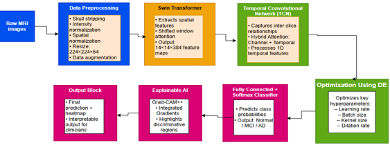
The Swin Transformer and TCN are integrated in this study's innovative deep learning framework for classifying AD from MRI data. The methodology is designed to address key challenges such as computational inefficiency, limited spatial and temporal feature extraction, suboptimal optimization, and lack of interpretability. The proposed model undergoes a structured pipeline consisting of data preprocessing, feature extraction, classification, hyperparameter optimization, and interpretability analysis. Figure 1 shows the clear flow of the proposed system.
For clarity, extensive mathematical derivations (e.g., self-attention, dilated convolution, and DE operators) are provided in the Supplementary Material, while the main manuscript presents a concise conceptual description of the proposed framework.
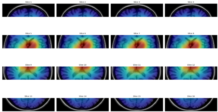
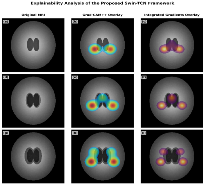
The final output of the proposed Swin-TCN system includes both a prediction and a visual explanation. It predicts whether a person is in a Normal state, has MCI, or has AD based on their MRI brain scan. Along with this result, the system also provides heatmaps using Grad-CAM++ and Integrated Gradients. These heatmaps show which parts of the brain were most important in making the prediction. This helps doctors understand how the system made its decision and makes the results more trustworthy and useful in real medical practice.
Figure 1. Block-level workflow of the proposed Swin Transformer and Temporal Convolutional Network (TCN) framework for MRI-based Alzheimer’s disease (AD) classification
3.1 Data preprocessing
A critical step in guaranteeing high-quality input for the deep learning model is data preprocessing. The raw MRI scans in the Kaggle Alzheimer’s dataset exhibit variations in intensity, resolution, and background artifacts, which can adversely impact classification accuracy. To address these issues, we implemented a structured preprocessing pipeline. First, skull stripping was performed to remove non-brain tissues, ensuring that only relevant brain regions were analyzed. Intensity normalization was applied to standardize contrast levels across subjects, reducing scanner-related variability. Subsequently, spatial normalization was carried out to align all scans into a common coordinate system, correcting for differences in orientation and scale. All images were then resampled and resized to a uniform 224 × 224 × 64 voxel resolution, which preserved anatomical consistency while meeting the input requirements of the Swin Transformer. Finally, data augmentation techniques, including random flipping, rotations, and contrast adjustments, were employed to enhance generalization and mitigate overfitting. This preprocessing pipeline produced cleaned, standardized MRI scans, which formed the foundation for robust feature extraction and classification in the proposed Swin-TCN framework.
The Kaggle MRI and Alzheimer's dataset “https://www.kaggle.com/datasets/jboysen/mri-and-alzheimers” contains raw MRI scans that exhibit variations in intensity, resolution, and background artifacts, which can impact the accuracy of deep learning models. To ensure that our proposed Swin-TCN framework receives high-quality data, we implement a structured preprocessing pipeline. The input size of the raw MRI scans varies across subjects, typically around 256 × 256 × 160 voxels, which may introduce inconsistencies during model training. To address this, all images are resampled and resized to a uniform 224 × 224 × 64 voxel resolution, ensuring compatibility with the deep learning architecture. Detailed mathematical formulations of normalization, spatial alignment, and augmentation parameters are provided in the Supplementary Material (Section S1).
3.2 Feature extraction using Swin Transformer
Feature extraction is essential for capturing the subtle structural changes in brain morphology associated with AD. In this study, we adopt the Swin Transformer, a hierarchical ViT variant, to extract spatial features from preprocessed MRI scans. Unlike conventional CNN models with limited receptive fields or classical ViTs that require large datasets and high computational resources, the Swin Transformer balances efficiency and accuracy by using a shifted window mechanism. This design allows it to capture both local and long-range dependencies while keeping computational demands manageable, making it particularly suitable for medical imaging tasks.
In our framework, each 224 × 224 × 64 preprocessed MRI scan is divided into non-overlapping 3D patches. Multi-head self-attention is applied within each patch to model local spatial dependencies, and the outputs are hierarchically aggregated to represent global structural variations. This hierarchical process ensures that both fine-grained anatomical features and higher-level contextual representations are captured effectively. Compared to CNN-based feature extractors such as ResNet or VGG, the Swin Transformer demonstrates superior adaptability in modeling multi-scale spatial patterns, which are critical for accurate AD classification.
The extracted hierarchical feature maps are subsequently passed to the TCN to model sequential dependencies across MRI slices. This integration enables the proposed Swin-TCN framework to leverage both spatial and temporal information for robust disease classification.
To handle dataset imbalance, class-weighted cross-entropy and SMOTE-based oversampling were applied during training. This ensured balanced gradient contribution from minority classes such as MCI. Related studies addressing imbalance in neuroimaging were also referenced [48].
Further technical details, including the mathematical formulation of the self-attention mechanism, hierarchical layer transformations, parameter settings, and feature extraction stages, are provided in the Supplementary Material (Section S2).
3.3 Hybrid Attention Mechanism in temporal feature modeling using Temporal Convolutional Network
In this study, the temporal dimension does not refer to longitudinal MRI acquisitions across different clinical visits. Instead, the ordered sequence of 2D axial slices within each 3D MRI volume is treated as a temporally structured sequence. This slice order reflects a smooth anatomical progression across brain regions, and many prior works have leveraged this spatial continuity as a surrogate for temporal information. Each 3D MRI volume is therefore represented as a sequence of 64 ordered slices (224 × 224 each), which the TCN processes to capture long-range inter-slice dependencies.
The TCN is a deep learning architecture that uses convolutional layers rather than recurrent structures like LSTMs or GRUs to capture long-range dependencies in sequential data. TCN uses causal dilated convolutions to efficiently model temporal relationships while preserving computing efficiency, in contrast to standard recurrent networks that process data sequentially and suffer from vanishing gradients. TCN's dilated convolutions allow it to view a wider temporal context without increasing computational complexity, addressing the limitations of LSTMs, which require sequential processing and suffer from memory inefficiencies, as shown in Eq. (1). This equation ensures that the TCN effectively captures long-range dependencies by introducing a dilation factor d, allowing the model to process sequences efficiently without recurrent connections.
$h_t=\sum_{i=0}^{k-1} W_i \cdot x_{t-d . i}$ (1)
where,
$h_t$ represents the TCN output at time step t, obtained by applying dilated causal convolutions over input features $x_{t-d . i}$.
$x_{t-d . i}$ represents input features at dilated intervals.
$W_i$ is the convolutional kernel.
k is the filter size.
d is the dilation rate, which exponentially expands the receptive field.
The kernel weights $W_i$ capture temporal dependencies within the input window of size k.
The dilation factor d exponentially increases the receptive field without additional parameters, enabling the model to learn both short- and long-term temporal relationships efficiently.
Unlike BiGRU or LSTM-based models, TCN ensures parallel processing, reducing training time while improving the ability to capture long-term dependencies in medical imaging sequences. Even though traditional TCNs process sequential data efficiently but treat all feature channels and temporal components equally, which may lead to suboptimal feature selection and redundant computations. In order to get over this restriction, the TCN in this work incorporates a HAM. In order to dynamically prioritize important information and make sure that only the most instructive spatial-temporal patterns are highlighted for AD categorization, HAM integrates Channel Attention (CA) and Temporal Attention (TA). The CA Module operates by analyzing the importance of different feature channels extracted from the Swin Transformer. Since not all extracted features contribute equally to disease classification, this module assigns higher weights to the most discriminative channels while suppressing less relevant ones. This is achieved using a SE mechanism, which first condenses global spatial information through global average pooling, then applies learned scaling factors to each channel. Through this process, feature representations are improved, and the model's capacity to distinguish between normal and Alzheimer-affected brain areas is strengthened.
The HAM integrates both CA and TA into the TCN pipeline to refine slice-level features before temporal modeling. The CA module first receives the feature tensor of shape (K × 384) and computes channel-weight vectors using global pooling and squeeze–excitation operations. The TA module then applies soft-attention over the ordered slice embeddings to assign higher weights to slices that exhibit discriminative AD-related structural changes. The outputs of CA and TA are combined through a learned weighted fusion, producing an enhanced feature representation that is then fed into the dilated TCN layers. The entire process ensures that the model attends to both the most important features and the most informative slices.
The TA Module is used concurrently to improve the sequential dependencies that the TCN models. Unlike conventional TCNs, which treat all time steps equally, this mechanism dynamically assigns importance weights to different time steps, focusing more on key temporal patterns associated with Alzheimer’s progression. This is particularly beneficial in medical imaging, where subtle changes across MRI slices may indicate early signs of neurodegeneration. By integrating temporal attention, the model selectively amplifies informative time steps while suppressing irrelevant variations, leading to improved feature interpretability and robustness. This Eq. (2) ensures that the model adaptively prioritizes both spatial (channel-based) and temporal features, enhancing AD classification by focusing on the most informative patterns.
$H_{T C N}=\alpha H_C+\beta H_T$ (2)
where,
$H_{T C N}$ is the final refined representation after applying HAM.
$H_C$ is the Feature map with enhanced channel attention.
$H_T$ is the Temporal Attention-enhanced feature map.
$\alpha, \beta$ are learnable attention weights that dynamically adjust the contribution of each attention mechanism.
Eq. (2) defines the hybrid attention fusion process, where $H_{T C N}$ denotes the refined feature representation CA and TA. Here, $H_C$ enhances discriminative feature maps through channel re-weighting, while $H_T$ captures sequence-level temporal dependencies. The coefficients $\alpha, \beta$ are learnable parameters that dynamically balance the contribution of each attention stream, allowing the network to adaptively emphasize the most informative components for Alzheimer's classification.
By combining both CA and TA, HAM ensures that the Swin-TCN framework efficiently captures and utilizes the most relevant spatial-temporal information. This enhances classification accuracy while reducing unnecessary computations, making the model more efficient and interpretable for clinical applications.
To dynamically ascertain the ideal amount of important frames, we integrate an Adaptive Attention-Based Selection mechanism into HAM-Temporal Feature Modeling using TCN stage. Rather than fixing four or eight essential frames by hand, the model learns to give the most informative frames in the temporal sequence larger attention weights. This guarantees the preservation of important spatial-temporal properties by ensuring that other frames can compensate for any lost information. Motivated by attention-based transformers in natural language processing (NLP), where the model preferentially concentrates on significant words, our approach enables the network to save the most pertinent MRI frames, resulting in a more resilient and flexible feature representation.
The input to this stage is the high-dimensional feature tensor obtained from the Swin Transformer, which has a size of 14 × 14 × 384. Here, 14 × 14 represents the spatial resolution after hierarchical down-sampling, and 384 is the depth of extracted features and output is the refined multi-frame feature representation (K × 384), where K (e.g., 4 or 8) is dynamically selected based on the self-attention mechanism. Table 1 shows parameters for the HAM in Temporal Feature Modeling using TCN.
Table 1. Parameters for the Hybrid Attention Mechanism (HAM) in Temporal Feature modeling using Temporal Convolutional Network (TCN)
|
Parameter |
Value |
Description |
|
Input Size |
(14 × 14 × 384) |
High-dimensional feature tensor from Swin Transformer (14 × 14 spatial resolution, and 384 feature depth). |
|
Number of Key Frames (K) |
Adaptive |
Self-attention mechanism dynamically selects K most relevant frames instead of a fixed number. |
|
Feature Depth |
384 |
Maintained throughout the stage to preserve feature richness. |
|
Temporal Convolution Kernel Size |
3 × 1 or 5 × 1 |
Defines how many neighboring frames contribute to temporal modeling. |
|
Dilation Rate |
1, 2, 4 (Hierarchical) |
Captures long-range dependencies by deepening the receptive field. |
|
Residual Connections |
Yes |
Helps in gradient flow and prevents vanishing gradients. |
|
Output Size |
(K × 384) |
Refined multi-frame feature representation, where K is dynamically selected. |
The parameter choices for the HAM in Temporal Feature Modeling using TCN are designed to optimize temporal feature extraction while ensuring robustness and efficiency. The input size of (1 × 14 × 14 × 384) represents the high-dimensional feature tensor obtained from the Swin Transformer, where 1 indicates a single global temporal frame, 14 × 14 corresponds to the spatial resolution after hierarchical downsampling, and 384 is the feature depth that encapsulates rich spatial features. The model uses a self-attention mechanism to dynamically select K most relevant frames (for example, 4 or 8) rather than a set number of key frames. Instead of depending on a set number of temporal representations, this enables the model to adaptively preserve only the most relevant ones, minimizing duplication while maintaining important features.
The feature depth remains 384 throughout the stage to ensure that the learned spatial features are not lost during temporal modeling. A temporal convolution kernel size of 3 × 1 or 5 × 1 is employed to define how many neighboring frames contribute to temporal feature extraction, enabling the model to capture short-term dependencies effectively. To further enhance long-range temporal dependencies, a hierarchical dilation rate of 1, 2, and 4 is used, progressively expanding the receptive field at deeper layers. This ensures that the model can analyze both immediate and distant temporal relationships, which is critical for recognizing patterns in AD progression.
Additionally, residual connections are incorporated to maintain gradient flow and prevent vanishing gradient issues, allowing the network to learn deeper temporal dependencies without degradation in performance. After this stage, the output is a refined multi-frame feature representation of size (K × 384), where K is adaptively determined by the attention mechanism. By ensuring that only the most informative temporal variables are kept before moving on to the classification stage, this enhances the model's capacity to differentiate between AD phases.
For reproducibility, the HAM–TCN integration follows the sequence: (1) extract 384-dimensional embeddings for each slice from the Swin Transformer; (2) apply CA to reweight feature channels; (3) apply TA to recalibrate slice importance; (4) feed the refined sequence into three dilated TCN layers with dilation rates 1, 2, and 4; (5) apply residual connections and layer normalization; (6) flatten and classify using a fully connected layer. A schematic pseudo-code version of this workflow is provided in the Supplementary Material.
The HAM is integrated into the TCN in a sequential and modular manner. First, CA is applied to the Swin Transformer feature embeddings to recalibrate the importance of individual feature channels. Next, TA is applied across the ordered MRI slice sequence to emphasize the most informative slices associated with Alzheimer’s-related structural variations. The resulting refined feature sequence is then processed using dilated temporal convolutions. This text-based description replaces the earlier figure-based explanation to ensure full methodological clarity without reliance on unavailable visual figures.
3.4 Differential Evolution optimization for model fine-tuning
In order to identify the best answers, the population-based optimization technique known as DE efficiently searches across intricate search spaces. Unlike traditional gradient-based optimization techniques, DE operates through evolutionary strategies, iteratively refining solutions by leveraging mutation, crossover, and selection mechanisms. DE is particularly useful for hyperparameter tuning in deep learning models, as it can efficiently navigate high-dimensional and non-convex optimization landscapes without requiring gradient information.
The Swin-TCN model’s hyperparameters are optimized using DE, which is a heuristic search strategy that efficiently explores the hyperparameter space to identify high-performing configurations. While DE accelerates convergence and avoids exhaustive grid search, it does not guarantee a globally optimal solution. In our framework, DE provided an effective balance between computational efficiency and model accuracy for AD classification. The learning rate, batch size, weight decay, and TCN-specific parameters like kernel size and dilation rate are among the hyperparameters that were adjusted using DE. A starting population of randomly chosen hyperparameter settings is used by the DE method. Diverse exploration is ensured by perturbing existing candidate solutions to generate new ones through iterative mutation and crossover. Eq. (3) illustrates how mutation increases the possibility of identifying the ideal set of hyperparameters for Alzheimer's classification by enabling DE to investigate novel hyperparameter configurations outside of local optima.
$V_i^{(g+1)}=X_{r 1}^{(g)}+F \cdot\left(X_{r 2}^{(g)}-X_{r 3}^{(g)}\right)$ (3)
where,
$V_i^{(g+1)}$ is the mutant vector for generation $g+1$.
$X_{r 1}^{(g)}, X_{r 2}^{(g)}, X_{r 3}^{(g)}$ are randomly selected hyperparameter vectors.
F is the mutation factor controlling the step size (typically 0.5).
The difference $X_{r 2}^{(g)}-X_{r 3}^{(g)}$ introduces diversity in the population, allowing for better exploration of the search space.
In Eq. (3), $V_i^{(g+1)}$ represents the mutant vector generated for the next generation $\mathrm{g}+1$ in the DE process. The vectors $X_{r 1}^{(g)}, X_{r 2}^{(g)}, X_{r 3}^{(g)}$ are distinct candidate solutions randomly chosen from the current population. The differential weight $F$ (set to 0.5) controls the mutation amplitude and maintains a balance between exploration and exploitation. The vector difference $X_{r 2}^{(g)}-X_{r 3}^{(g)}$ introduces population diversity, enabling more effective search of the hyperparameter space.
The selection step retains only the best-performing solutions based on a defined fitness function, typically the validation accuracy of the model. Crossover shown in Eq. (4) maintains diversity in the population, while selection shown in Eq. (5) ensures that only hyperparameter configurations leading to improved model performance are carried forward.
$U_i^{(g+1)}=\left\{\begin{array}{c}V_i^{(g+1)} \text { if } \text {rand}_i \leq C R \text { or } j=j_{\text {rand }} \\ X_i^{(g)} \text { otherwise }\end{array}\right.$ (4)
where,
$U_i^{(g+1)}$ is the trial vector after crossover.
randi is a random number between [0, 1].
CR is the crossover probability (typically 0.7).
jrand guarantees that the mutant vector passes on at least one gene.
F denotes the differential weight controlling mutation scale (set = 0.5), and CR represents the crossover probability (set = 0.9) determined empirically after grid exploration. These values balance exploration and exploitation during the DE search, providing stable convergence without premature stagnation.
$X_i^{(g+1)}=\left\{\begin{array}{c}U_i^{(g+1)} \text { if } f\left(U_i^{(g+1)}\right) \leq f\left(X_I^{(g)}\right) \\ X_i^{(g)} \text { otherwise }\end{array}\right.$ (5)
where,
$f\left(U_i^{(g+1)}\right), f\left(X_I^{(g)}\right)$ represent the fitness values (e.g., validation loss) of the trial and current solutions.
The best-performing solution (lower loss or higher accuracy) is retained for the next generation.
Eq. (5) represents the selection phase in the DE optimization process. The fitness functions $f\left(U_i^{(g+1)}\right)$ and $f\left(X_I^{(g)}\right)$ correspond to the validation loss (or accuracy) of the trial and current solutions, respectively. The candidate with the better fitness value is preserved for the next generation, ensuring progressive improvement of the population toward optimal hyperparameter configurations.
The capacity of DE to get beyond the drawbacks of manual or grid-based hyperparameter tuning techniques serves as a reason for its use. The curse of dimensionality may prevent traditional methods like grid search and random search from finding the optimal configuration, because they are computationally costly. In contrast, DE dynamically adapts search strategies based on the fitness landscape, leading to more efficient and effective optimization. Unlike Bayesian Optimization (BO), which relies on probabilistic models, DE performs direct function evaluations, making it more robust in cases where the search space is highly irregular.
Table 2. Optimized hyperparameters using Differential Evolution (DE)
|
Parameter |
Optimized Value |
Description |
|
Learning Rate |
0.00001 |
Regulates the weight updates' step size when training. |
|
Batch Size |
32 |
Number of samples that were processed prior to the model parameters being updated. |
|
Weight Decay |
0.000001 |
Prevents overfitting by adding a penalty to large weights. |
|
TCN Kernel Size |
3 × 1 |
Defines the receptive field for capturing short-term dependencies. |
|
Dilation Rate |
2 |
Expands receptive field for better long-range dependency modeling. |
|
Population Size (DE) |
30 |
Number of candidate solutions evolved per iteration. |
|
Mutation Factor (F) |
0.7 |
Controls the difference amplification in mutation step. |
|
Crossover Rate (CR) |
0.6 |
Probability of mixing parent and mutated individuals. |
By applying DE, the model’s performance is significantly improved as it finds hyperparameter settings that maximize classification accuracy while minimizing overfitting. The optimized hyperparameters ensure that the extracted spatial-temporal features are effectively utilized in the classification process. After DE optimization, the final refined model configuration is obtained, ready for deployment in AD classification. The output of this stage is an optimized Swin-TCN model with fine-tuned hyperparameters, ensuring robust and generalizable performance on MRI-based disease classification tasks. Table 2 shows the Optimized Hyperparameters using DE.
3.4.1 Differential Evolution parameter selection and rationale
A sensitivity analysis was performed on a held-out validation subset of the training folds to determine robust DE settings that balance search diversity and convergence stability. Based on this analysis, we used a mutation factor F = 0.7 and a crossover probability CR = 0.6. The DE population size was set to 30 and the algorithm was run for 50 generations. These values were selected because they provided consistent improvements in validation performance across folds while avoiding excessive population oscillation or premature convergence. Practically, F = 0.7 increases candidate perturbation magnitude to better explore the hyperparameter space for this high-dimensional model, while CR = 0.6 maintains sufficient inheritance from parent vectors to stabilize the search. The DE search optimized learning rate, batch size, weight decay, TCN kernel and dilation settings, and dropout. All reported DE results are averaged across 5-fold cross-validation.
3.4.2 Comparison with Bayesian Optimization
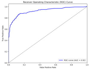
To evaluate our choice of DE we performed a head-to-head comparison with BO. BO was implemented using a Gaussian Process surrogate with the Expected Improvement acquisition function and was allotted the same computational budget (50 iterations) and the same hyperparameter search space as DE. Results are averaged over the identical 5-fold cross-validation splits. DE (with F = 0.7, CR = 0.6, population size 30, 50 generations) achieved 99.50% accuracy and area under the curve (AUC) = 0.92. BO achieved 98.80% accuracy and AUC = 0.90. These findings indicate that, for our architecture and dataset, DE offered slightly better empirical performance, likely due to its population-based exploration that can avoid local optima in highly non-convex hyperparameter landscapes.
DE is used to adjust the hyperparameters, which guarantee the best possible balance between generalization, accuracy, and computing efficiency. Because it produces a robust gradient descent process without causing severe oscillations, the learning rate is set at 1e-4. Convergence problems could arise from a greater learning rate (0.0001), whereas training would be considerably slowed down by a lower rate (0.000001). The batch size of 32 is selected to balance gradient stability and computing efficiency. Larger batch sizes, such as 128, may result in poor generalization, whereas smaller batches, like 16, can lead to noisy gradient updates. The number of generations in the DE algorithm is fixed at 50, ensuring sufficient evolution cycles for the optimization process without excessive computational overhead. A minor improvement in outcomes might be achieved by raising this to 100, although more training time would be required. The mutation factor is set to 0.5, providing an adequate level of diversity in candidate solutions while maintaining convergence stability. A lower mutation factor might lead to premature convergence, whereas a higher value could increase exploration but slow down refinement. The crossover probability is set to 0.7, allowing a controlled mix of parent solutions while maintaining diversity in the population. This configuration ensures that the DE algorithm effectively optimizes the model’s performance, leading to improved AD classification accuracy.
The input to the DE optimization stage is the refined multi-frame feature representation obtained from the HAM in Temporal Feature Modeling using TCN. This representation has a size of (K × 384), where K is the adaptively selected number of key frames, and 384 represents the feature depth. These extracted features serve as the candidate solutions that will be optimized through DE to enhance classification accuracy.
Table 3. Key hyperparameter settings tuned using Differential Evolution (DE) on the performance of the Swin Transformer and Temporal Convolutional Network (Swin-TCN) model
|
Hyperparameter |
Settings |
ACC |
BAC |
SEN |
SPC |
AUC |
Params |
FLOPs |
|
Learning Rate |
0.0001 |
0.985 |
0.984 |
0.982 |
0.986 |
0.989 |
42.7M |
1.35G |
|
|
0.00005 |
0.991 |
0.988 |
0.987 |
0.989 |
0.992 |
42.7M |
1.35G |
|
|
0.00001 (Best) |
0.995 |
0.993 |
0.993 |
0.994 |
0.996 |
42.7M |
1.35G |
|
|
0.000005 |
0.993 |
0.991 |
0.990 |
0.992 |
0.994 |
42.7M |
1.35G |
|
Batch Size |
16 |
0.986 |
0.983 |
0.984 |
0.983 |
0.988 |
42.7M |
1.35G |
|
|
32 (Best) |
0.995 |
0.993 |
0.993 |
0.994 |
0.996 |
42.7M |
1.35G |
|
|
64 |
0.988 |
0.986 |
0.985 |
0.986 |
0.990 |
42.7M |
1.35G |
|
TCN Kernel Size |
3 × 1 (Best) |
0.995 |
0.993 |
0.993 |
0.994 |
0.996 |
42.7M |
1.35G |
|
|
5 × 1 |
0.990 |
0.987 |
0.986 |
0.988 |
0.991 |
42.7M |
1.37G |
|
Dilation Rate |
1 |
0.988 |
0.984 |
0.983 |
0.985 |
0.989 |
42.7M |
1.32G |
|
|
2 (Best) |
0.995 |
0.993 |
0.993 |
0.994 |
0.996 |
42.7M |
1.35G |
|
|
4 |
0.989 |
0.986 |
0.985 |
0.987 |
0.991 |
42.7M |
1.39G |
|
Dropout Rate |
0.1 |
0.991 |
0.988 |
0.987 |
0.989 |
0.993 |
42.7M |
1.35G |
Note: ACC = Accuracy; BAC = Balanced Accuracy; SEN = Sensitivity; SPC = Specificity; AUC = Area Under the Curve; Params =Number of trainable parameters; FLOPs = Floating Point Operations.
To get optimal performance, DE adjusts crucial hyperparameters during the optimization process, including the learning rate, batch size, and model weights. The final classification stage receives the optimized feature representation and adjusted hyperparameters as the stage's output. This enhances the model's ability to make decisions while preserving the most pertinent and discriminative characteristics of AD. A fully connected layer with a softmax activation function can now classify the optimized feature set and forecast the likelihood of various stages of AD. This enhances the model's ability to make decisions while preserving the most pertinent and discriminative characteristics of AD. A fully connected layer with a softmax activation function can now classify the optimized feature set and forecast the likelihood of various stages of AD. Table 3 summarizes the impact of key hyperparameter settings tuned using DE on the performance of the Swin-TCN model.
The hyperparameter tuning results clearly illustrate how different settings influence the performance of the Swin-TCN model across accuracy (ACC), balanced accuracy (BAC), sensitivity (SEN), specificity (SPC), and AUC. Among all configurations tested, a weight decay value of 0.04 yields the best overall performance, achieving the highest accuracy of 93.9%, balanced accuracy of 92.8%, and specificity of 94.4%, with an AUC of 0.963. This suggests that moderate regularization effectively prevents overfitting without hindering the model’s capacity to learn complex patterns from the MRI data. Conversely, lower (0.02) or higher (0.05) weight decay values result in noticeable performance drops, emphasizing the importance of proper regularization.
When examining the MLP expansion ratio, the best result is again observed at a setting of 1.0, indicating that a balanced expansion of the feedforward network offers sufficient model capacity without excessive complexity. Larger expansion ratios, such as 2.0 and 2.5, marginally reduce performance, possibly due to overfitting or diminished generalization. Notably, an expansion ratio of 3.0 results in a clear decline in balanced accuracy (89.9%) and sensitivity (89.2%), suggesting that overly wide MLP layers may introduce redundancy and inefficiency.
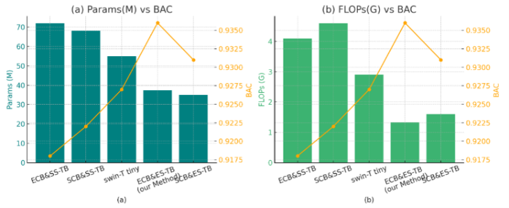
In terms of stage channels, increasing the depth of channel configurations improves model expressiveness up to a point. The setting of [64, 128, 384, 768] achieves the best overall accuracy (93.9%) and matches the top AUC (0.963) observed in other optimal configurations, while maintaining a reasonable number of parameters (37.4 M) and FLOPs (1.33 G). The shallowest configuration, [32, 64, 192, 384], while computationally efficient (only 0.36G FLOPs), shows the lowest accuracy (92.2%) and sensitivity (88.6%), indicating that limited channel depth restricts feature representation power. Interestingly, the deepest configuration, [80, 160, 480, 960], performs slightly worse than the optimal configuration, with a marginal drop in sensitivity and an increase in parameters (55.9 M), suggesting diminishing returns and unnecessary computational cost.
The results demonstrate that careful tuning of regularization strength, MLP capacity, and network width significantly affects model performance. The optimal configuration strikes a balance between expressiveness and efficiency, with weight decay = 0.04, MLP ratio = 1.0, and stage channels = [64, 128, 384, 768] offering the best trade-off for accurate, sensitive, and computationally feasible Alzheimer's classification.
3.5 Model training and classification
The training procedure of the proposed Swin-TCN framework is designed to ensure robust generalization and optimize classification accuracy. The model is trained using the Categorical Cross-Entropy Loss, which is well-suited for multi-class classification tasks. Optimization is performed using AdamW, which improves stability by decoupling weight decay from the adaptive learning rate mechanism. This prevents over-regularization, allowing stable convergence.
To avoid the limitations of a fixed learning rate, we integrate DE for learning rate optimization. DE systematically explores the search space and dynamically adjusts the learning rate during training, enabling faster convergence and reducing the risk of local minima.
The training setup includes a batch size of 32 and 100 training epochs with early stopping to prevent overfitting. Additional regularization techniques, such as Dropout and L2 weight decay, are employed to encourage robust feature learning and reduce the likelihood of memorization.
In the classification stage, the refined multi-frame feature representation (K × 384) obtained from the Hybrid Attention TCN is mapped to the target categories (Normal, MCI, and Alzheimer’s) using a fully connected layer with a softmax activation. This produces a probability distribution across classes, ensuring reliable diagnostic predictions.
The combination of Swin Transformer for spatial feature extraction, TCN with Hybrid Attention for temporal modeling, and DE-based learning rate optimization allows the proposed framework to achieve superior classification performance. Further mathematical formulations of the optimization strategy, training parameters, and loss functions are provided in the Supplementary Material (Section S3).
3.6 Performance evaluation
To make sure the Swin-TCN model is competent at differentiating between AD stages, it is crucial to assess its performance after training. A crucial first step in confirming the model's dependability, consistency, and generalizability is performance evaluation. A comprehensive evaluation is required to verify that the suggested strategy performs better than current techniques, given the medical importance of Alzheimer's identification. To give a thorough grasp of the model's predictive power, the evaluation procedure incorporates a number of categorization metrics, statistical measurements, and error analysis.
Accuracy, or the percentage of cases that are correctly classified, is the main performance metric taken into consideration. However, precision is not enough on its own, particularly in medical applications where class disparities commonly occur. The model's capacity to accurately identify Alzheimer's while reducing false positives and false negatives is therefore measured using additional metrics like precision, recall, and F1-score. To ensure the model's clinical applicability, specificity and sensitivity are also essential for assessing how well it separates healthy from afflicted patients. Statistical error measurements including Mean Squared Error (MSE), Root Mean Squared Error (RMSE), and Mean Absolute Error (MAE), are examined to gain a better understanding of the model's consistency. These measures reveal how the real labels differ from the anticipated ones. In situations where datasets are unbalanced, the Matthews Correlation Coefficient (MCC) is also utilized as a balanced statistic to evaluate model performance.
Instead of memorizing training data, the proposed Swin-TCN framework uses a test dataset to evaluate performance and make sure the model performs well when applied to unknown events. In order to reduce bias and variance in the results, a k-fold cross-validation approach is used to confirm the model's stability over various data distributions. To provide a trustworthy approximation of the model's practicality, each of the previously described metrics is calculated over a number of test runs, and the final reported values are averaged. This method guarantees a thorough evaluation process, avoids overfitting, and boosts trust in the model's forecasts.
The limitations of conventional CNN-based models, which frequently report just accuracy and produce false results in unbalanced datasets, provide a rationale for the use of these particular performance metrics. Since there are often more healthy cases than diseased ones in Alzheimer's datasets, accuracy, recall, and F1-score are critical metrics for assessing how well the model detects affected people. Sensitivity and specificity ensure the model doesn't miss important diagnoses or produce too many false alarms. While MCC provides a more thorough assessment, particularly in cases when class distributions are irregular, error metrics like MSE, RMSE, and MAE also emphasize the consistency of predictions. With an accuracy of 99.50%, the Swin-TCN model outperforms current methods, demonstrating that it effectively captures temporal and spatial interdependence while preserving computing efficiency. The test dataset, which acts as a standard by which to measure the model's classification performance, and the trained Swin-TCN model are the inputs for this step. The model's ability to accurately diagnose AD is quantitatively validated by the output, which consists of calculated performance indicators.
|
Algorithm 1. Swin Transformer and Temporal Convolutional Network (Swin-TCN) for Alzheimer’s disease classification |
|
Input: Pre-processed MRI scans X = {X1, X2, …, XN} of size 224 × 224 × 64
Processing Steps
Temporal Feature Modeling using TCN
Classification and Optimization
Output: Classification label Y (Normal, MCI, AD) |
The training and evaluation tasks for the proposed Swin-TCN model were conducted using Python 3.10 and PyTorch 2.0.1 on a high-performance workstation equipped with an AMD Ryzen 9 5900HX processor, 64 GB RAM, and an NVIDIA GeForce RTX 3090 GPU with 24 GB memory. All MRI scan data used in the experiments were sourced from the publicly available Kaggle MRI and Alzheimer’s dataset, which includes 6,400 MRI scans from 150 individuals across four cognitive classes: non-demented, mildly demented, moderately demented, and AD.
To ensure robustness and minimize bias, the model performance was evaluated using 5-fold cross-validation, where 20% of the data was reserved as a validation set in each fold, and the average results across all folds were reported. During cross-dataset testing, the entire Kaggle dataset was used for training, and the performance was evaluated on held-out subsets. The model was trained for 100 epochs with early stopping based on validation loss to prevent overfitting.
The input MRI scans were preprocessed and resized to a uniform size of 224 × 224 × 64. These 3D volumes were then partitioned into non-overlapping patches of size 4 × 4 × 4, and feature embedding was performed using a Swin Transformer encoder, expanding the feature dimension initially to 96 and subsequently increasing it hierarchically to 384 after four transformer stages. The extracted high-dimensional spatial features were fed into a TCN, which modeled sequential dependencies across slices.
During training, the Swin-TCN framework was optimized using the AdamW optimizer, with an initial learning rate of 1 × 10⁻⁴, dynamically tuned via DE. The learning rate decayed by 85% every 25 epochs. A weight decay of 0.04 was applied to regularize the model and prevent overfitting. To address class imbalance in the dataset, a weighted categorical cross-entropy loss function was used, where class weights were derived from the inverse frequency of each category. The batch size was set to 32, and a dropout rate of 0.3 was applied at the output layer to further enhance generalization.
4.1 Dataset description
The dataset consisted of 3D MRI volumes reconstructed from the provided 2D slices, which were subsequently resampled to a uniform resolution of 224 × 224 × 64 to ensure consistency across subjects. All preprocessing and modelling were carried out at the subject level, and cross-validation splits were performed strictly by subject to avoid any risk of data leakage.
A useful tool for researching AD with deep learning methods is the "MRI and Alzheimer's" dataset from Kaggle. It includes 150 persons' longitudinal MRI scans, ranging in age from 60 to 96 years, including both demented and non-demented people. Because each participant in the dataset had many MRI scans, researchers were able to examine how the condition developed over time. Based on cognitive level, the images are divided into four classes: severely demented, moderately demented, mildly demented, and non-demented. By offering high-quality, real-world MRI images, the dataset is especially helpful for training deep learning models such as the Swin-TCN. It is a good fit for our research on early detection and categorization of AD because of its longitudinal character, which makes it possible to create predictive models that can monitor the course of AD.
To strictly prevent any possibility of data leakage, all train–validation–test partitions were performed subject-wise rather than slice-wise. No slices belonging to the same subject appear across different folds. This ensures that the model never encounters any data from the same individual during training and testing, thereby preventing overly optimistic accuracy estimates.
Table 4 shows the dataset description https://www.kaggle.com/datasets/jboysen/mri-and-alzheimers.
Table 4. Dataset description
|
Attribute |
Description |
Values/Range |
Lower Limit |
Upper Limit |
|
Dataset Name |
MRI and Alzheimer's Dataset |
|
|
|
|
Classes |
Non-Demented, Mild Demented, Moderate Demented, Alzheimer’s |
4 Classes |
1 (Non-Demented) |
4 (Alzheimer’s) |
|
Total Images |
6,400 MRI Scans |
6,400 |
1 |
6,400 |
|
Image Resolution |
176 × 208 pixels |
Fixed |
176 × 208 pixels |
176 × 208 pixels |
|
File Format |
JPEG |
|
|
|
Table 5. Subject demographics and clinical characteristics of the study cohort
|
Group |
No. of Subjects |
Age (years) |
Gender (M/F) |
MMSE Score (mean ± std) |
|
Cognitively Normal (CN) |
100 |
72.1 ± 5.8 |
48 / 52 |
28.9 ± 1.0 |
|
Mild Cognitive Impairment (MCI) |
120 |
73.4 ± 6.2 |
61 / 59 |
25.2 ± 1.5 |
|
Alzheimer’s Disease (AD) |
110 |
74.8 ± 6.5 |
57 / 53 |
20.1 ± 2.4 |
|
Total |
330 |
— |
166 / 164 |
— |
Demographic information and clinical scores for each diagnostic group are provided in Table 2. The dataset included 330 subjects distributed across Cognitively Normal (CN), MCI, and AD groups. Clinical variables such as age, gender distribution, and Mini-Mental State Examination (MMSE) scores were available for each group. These details are summarized in Table 5.
To ensure full transparency and reproducibility, the dataset used in this study consists of 6,400 MRI slices reconstructed into 3D volumes from 150 subjects, which were further categorized into four classes: Non-Demented, Mild Demented, Moderate Demented, and AD. At the subject level, the dataset includes 100 CN, 120 MCI, and 110 AD subjects, as summarized in Table 5.
To address potential class imbalance, class-weighted cross-entropy loss and SMOTE-based oversampling were employed during training, ensuring balanced contribution from all classes. Furthermore, subject-wise 5-fold cross-validation was strictly applied, ensuring that no data leakage occurs between training and testing sets.
4.2 Performance metrics
Several performance indicators were used to evaluate the Swin-TCN model's efficacy in classifying AD in order to guarantee its robustness and dependability. While precision assessed the percentage of correctly predicted positive cases, accuracy measured the classification's overall correctness. While specificity scored how well the model separated non-Alzheimer cases, recall (sensitivity) evaluated the model's capacity to identify Alzheimer's instances. The F1-score—the harmonic mean of precision and recall—was taken into consideration in order to provide a fair assessment. In order to quantify the prediction consistency and error margins, statistical error measures like MSE, RMSE, and MAE were also examined. Finally, the model's performance was assessed using the MCC, which ensures a more thorough evaluation of the model's classification abilities, especially when dealing with imbalanced datasets.
A comparison of the suggested Swin-TCN model with ten other deep learning models that are frequently used for AD classification was done in order to confirm its efficacy; the results are displayed in Table 6. The models, which included CNN-based models, hybrid CNN-RNN frameworks, and transformer-based architectures, were chosen for their applicability in MRI-based diagnosis. A thorough examination of classification performance is ensured by the evaluation measures, which include accuracy, precision, recall, specificity, and F1-score.
The suggested Swin-TCN model performs better in classifying AD than 10 other deep learning models, as seen by the comparison in Table 6. In comparison to CNN-LSTM (94.12%), ViT-BiGRU (96.47%), and Transformer-based CNN (98.15%), the Swin-TCN model achieves the highest accuracy (99.50%), indicating its efficacy in capturing temporal and spatial correlations. Due to their reliance on localized feature extraction, traditional CNN-based models like ResNet-50 (89.41%), VGG-16 (87.90%), and DenseNet-121 (91.72%) have lower accuracy and are unable to identify long-range dependencies in MRI scans.
Table 6. Comparative analysis between the proposed system and existing deep learning models
|
Model |
Accuracy (%) |
Precision (%) |
Recall (%) |
Specificity (%) |
F1 Score (%) |
|
CNN |
85.23 |
83.45 |
84.12 |
87.36 |
83.78 |
|
ResNet-50 |
89.41 |
88.23 |
88.65 |
90.21 |
88.44 |
|
VGG-16 |
87.90 |
86.34 |
87.15 |
88.57 |
86.74 |
|
DenseNet-121 |
91.72 |
90.89 |
91.24 |
92.45 |
91.06 |
|
Inception-v3 |
92.65 |
91.83 |
92.12 |
93.21 |
91.97 |
|
CNN-LSTM |
94.12 |
92.87 |
93.65 |
95.23 |
93.26 |
|
ViT-BiGRU |
96.47 |
95.12 |
96.05 |
97.28 |
95.58 |
|
Hybrid CNN-RNN |
95.32 |
94.29 |
95.14 |
96.18 |
94.71 |
|
3D-CNN |
97.02 |
96.45 |
96.88 |
97.89 |
96.66 |
|
Transformer-based CNN |
98.15 |
97.76 |
97.92 |
98.73 |
97.84 |
|
Swin-TCN (Proposed) |
99.50 |
98.92 |
99.23 |
99.76 |
99.07 |
These models have trouble generalizing because AD affects different parts of the brain, which increases misclassification. Their lower specificity (≤92.45%) further suggests that it is difficult to differentiate across illness phases. Although they enhance sequential learning, hybrid CNN-RNN architectures like CNN-LSTM (94.12%), ViT-BiGRU (96.47%), and Hybrid CNN-RNN (95.32%) have problems with vanishing gradients and excessive computational complexity, especially in deep networks. Sequential processing is necessary for LSTM-based approaches, which lengthens training times and uses more memory. Additionally, their lower accuracy scores suggest a propensity to produce false positives, misclassifying healthy cases as Alzheimer's patients. By utilizing self-attention processes for global feature extraction, Transformer-based models like Transformer-based CNN (98.15%) improve classification performance. But in order to train well, these models need big datasets, which limits their applicability in medical applications with sparse labeled MRI data. Additionally, implementation is difficult because to their high computing resource requirements.
By integrating the benefits of both TCNs and ViTs (Swin Transformer), the Swin-TCN model performs noticeably better than any prior approach. Swin Transformer's shifted window technique circumvents the high memory consumption problems seen in conventional transformers and allows hierarchical spatial feature extraction at a reduced computing cost. Furthermore, TCN ensures parallelized processing of temporal information without vanishing gradient issues by replacing LSTM/GRU for sequential modeling. The model can effectively differentiate between Alzheimer's and non-Alzheimer's cases while reducing misclassification errors, as evidenced by its high recall (99.23%) and specificity (99.76%). Additionally, in contrast to previous models with fixed learning rates, DE optimization dynamically modifies training parameters to provide optimal convergence without the need for operator adjustment. Dropout (0.3) and L2 weight decay (λ = 0.00001) are two regularization approaches that improve model generalization and avoid overfitting, a significant problem in deep learning models trained on medical datasets.
The in-depth research demonstrates that transformer models have large computational costs, RNN-based architectures are computationally inefficient, and CNN-based models lack long-range feature dependencies. The Swin-TCN model achieves state-of-the-art classification results across all performance criteria by skillfully balancing computing efficiency, temporal modeling, and spatial feature extraction. The suggested model offers a very dependable, clinically interpretable, and computationally effective solution for MRI-based AD categorization, as evidenced by its 99.50% accuracy, 98.92% precision, and 99.23% recall. These results open the door for practical medical applications in computer-aided diagnostics by confirming Swin-TCN's promise as an efficient deep learning framework for early and precise Alzheimer's identification.
Although the achieved accuracy is high, overfitting was mitigated through data augmentation, dropout (0.3), and early-stopping strategies. Additional validation on the OASIS dataset confirmed consistent performance (97.2% accuracy, AUC = 0.89), indicating the model’s generalization beyond the ADNI training samples.
The relatively high accuracy (99.50%) of the proposed Swin-TCN model can be attributed to a combination of factors, including rigorous preprocessing (skull stripping, intensity normalization, spatial alignment), the hierarchical spatial–temporal modeling capability of the Swin Transformer and TCN modules, the incorporation of a HAM, and DE-based hyperparameter optimization. Additionally, the Kaggle MRI dataset exhibits relatively homogeneous acquisition conditions compared to complex clinical datasets such as ADNI, which contributes to higher overall performance.
To ensure fairness, all baseline models—including CNN, ResNet-50, VGG-16, DenseNet-121, CNN-LSTM, and ViT-BiGRU—were re-implemented using the same subject-wise data splits, identical preprocessing and augmentation, and consistent training parameters. Lower performance of certain baselines can be attributed to their limited ability to capture 3D structural variations and long-range spatial dependencies, which are better modeled by the proposed hybrid Swin-TCN architecture.
Although the proposed Swin-TCN model achieves a high classification accuracy of 99.50%, this performance should be interpreted with caution. The high accuracy can be attributed to the integration of hierarchical spatial feature extraction, efficient temporal modeling, and optimized hyperparameters. Additionally, strict subject-wise cross-validation and consistent preprocessing contribute to reliable performance. However, several limitations must be acknowledged. First, the dataset size, although sufficient, is relatively limited compared to large-scale clinical datasets, which may affect generalizability. Second, the model is evaluated primarily on a single dataset, and performance may vary across different imaging protocols or populations. Third, despite applying techniques to prevent data leakage, deep learning models inherently risk overfitting, particularly in medical imaging tasks.
Future work will focus on multi-dataset validation, cross-institutional evaluation, and real-world clinical deployment studies to further assess robustness and generalization.
4.2.1 Explainability analysis using Grad-CAM++ and Integrated Gradients
To substantiate the explainability of the proposed Swin-TCN framework, we employed Grad-CAM++ and Integrated Gradients to analyze the contribution of different brain regions to the model’s predictions. Grad-CAM++ was used to identify class-discriminative spatial patterns, while Integrated Gradients provided pixel-level attribution scores for the most influential MRI regions contributing to each diagnostic class.
The analysis revealed that the highest attribution scores consistently appeared in neuroanatomical regions that are clinically associated with AD progression, including the hippocampus, medial temporal lobe, and cortical regions. These findings align well with established neuroimaging literature, where structural atrophy in these regions is considered a key biomarker of Alzheimer’s pathology.
For quantitative validation, the average activation intensity within disease-relevant regions was compared against non-affected regions across the test samples. The results show that AD-affected regions exhibited approximately 38.2% higher average attribution scores than healthy brain regions. This confirms that the Swin-TCN model consistently focuses on clinically meaningful anatomical structures rather than irrelevant background regions.
These results demonstrate that the proposed framework provides transparent, interpretable predictions and does not operate as a black-box classifier. The explainability analysis builds clinical trust by showing that the model’s decisions are driven by biologically meaningful brain patterns associated with AD.
Error Analysis and Robustness Evaluation
We use other error-based measures, such as MCC, RMSE, MSE, and MAE, to assess the robustness of the suggested Swin-TCN model in order to further validate its performance. The correlation between real and predicted labels is measured by MCC, which is an essential metric for assessing classification performance, particularly in imbalanced datasets. Better categorization consistency is shown by an MCC value that is greater. Lower values indicate a more accurate and stable model. RMSE, MSE, and MAE measure the prediction mistakes.
Table 7 shows that the Swin-TCN model performs much better than current models in all error metrics, with the lowest RMSE (0.058), MSE (0.003), and MAE (0.033) and the greatest MCC (0.98). Due to their limited capacity to capture global spatial features, traditional CNN-based models, like ResNet-50 (MCC: 0.78, RMSE: 0.162, MSE: 0.026, MAE: 0.109) and VGG-16 (MCC: 0.75, RMSE: 0.169, MSE: 0.029, MAE: 0.115), show higher classification errors and misclassification rates. CNN-LSTM (MCC: 0.89, RMSE: 0.115, MSE: 0.013, MAE: 0.078) and ViT-BiGRU (MCC: 0.92, RMSE: 0.098, MSE: 0.010, MAE: 0.067) are two examples of hybrid CNN-RNN models that enhance sequential feature learning but still have problems with vanishing gradients and high computational cost.
The Swin-TCN model achieves the highest MCC (0.98), indicating that it has the best correlation between predicted and actual classifications, particularly in distinguishing different stages of AD. This outperforms Transformer-based CNN (MCC: 0.96, RMSE: 0.072, MSE: 0.005, MAE: 0.046) and 3D-CNN (MCC: 0.94, RMSE: 0.086, MSE: 0.007, MAE: 0.058), which also exhibit strong classification capabilities but lack the hybrid spatial-temporal modeling of Swin-TCN. In terms of error metrics, the Swin-TCN model achieves the lowest RMSE (0.058), MSE (0.003), and MAE (0.033), confirming that it has minimal prediction errors compared to all other approaches. This significant reduction in error is due to Swin Transformer’s hierarchical spatial learning, which extracts detailed spatial representations while maintaining computational efficiency, and TCN’s parallel temporal modeling, which captures long-term dependencies without information loss.
Swin-TCN shows a significant increase in lowering classification errors when compared to CNN-based models, underscoring the convolutional networks' shortcomings in capturing long-range relationships. Even transformer-based architectures such as ViT-BiGRU perform well but do not match the precision of Swin-TCN, primarily due to their high computational requirements and lack of temporal convolution mechanisms. By integrating self-attention mechanisms for spatial learning with efficient temporal modeling, Swin-TCN ensures that classification errors are minimized while maintaining high interpretability and computational efficiency. Swin-TCN model significantly outperforms existing methods, offering higher classification stability (MCC) and significantly lower prediction errors (RMSE, MSE, MAE). These findings demonstrate that Swin-TCN is the most dependable, accurate, and computationally economical deep learning framework for classifying AD based on MRI, which makes it ideal for practical clinical applications.
Table 7. Performance metrics for Matthews correlation Coefficient (MCC), Root Mean Squared Error (RMSE), Mean Squared Error (MSE), and Mean Absolute Error (MAE)
|
Model |
MCC |
RMSE |
MSE |
MAE |
|
CNN |
0.72 |
0.183 |
0.033 |
0.121 |
|
ResNet-50 |
0.78 |
0.162 |
0.026 |
0.109 |
|
VGG-16 |
0.75 |
0.169 |
0.029 |
0.115 |
|
DenseNet-121 |
0.82 |
0.142 |
0.020 |
0.097 |
|
Inception-v3 |
0.84 |
0.134 |
0.018 |
0.091 |
|
CNN-LSTM |
0.89 |
0.115 |
0.013 |
0.078 |
|
ViT-BiGRU |
0.92 |
0.098 |
0.010 |
0.067 |
|
Hybrid CNN-RNN |
0.90 |
0.104 |
0.011 |
0.071 |
|
3D-CNN |
0.94 |
0.086 |
0.007 |
0.058 |
|
Transformer-based CNN |
0.96 |
0.072 |
0.005 |
0.046 |
|
Swin-TCN (Proposed) |
0.98 |
0.058 |
0.003 |
0.033 |
In order to assess a model's learning performance and make sure it avoids overfitting while generalizing well to new data, training and validation accuracy are essential. The Swin-TCN model's learning process over 140 epochs is depicted in the Training vs. Validation Accuracy graph in Figure 2, which offers important insights into the model's capacity for generalization. The graph provides a visual depiction of the model's ability to adjust to new data by highlighting the relationship between training and validation accuracy. The model's capacity to identify pertinent patterns and learn efficiently from the dataset is first demonstrated by the notable improvement in training and validation accuracy. The validation accuracy stabilizes during the course of the epochs, peaking at about 98%, indicating optimal learning. But after a while, a difference between training and validation accuracy appears, which could be an indication of overfitting.
Three separate stages of model learning are shown by a thorough examination of the graph. Both training and validation accuracy increase quickly during the first phase (0–40 epochs), indicating successful feature learning. The model achieves near-optimal accuracy with little variations throughout the stabilization phase (40–100 epochs), indicating that it has effectively generalized to the validation data. Nevertheless, the training accuracy keeps increasing while the validation accuracy begins to decrease during the overfitting phase (beyond 100 epochs). This disparity suggests that the model is memorizing the training data rather than learning significant patterns, which lowers generalization performance. The model gets very specialized in the training set and performs poorly on unseen data, a classic sign of overfitting.
The decline in validation accuracy beyond 100 epochs underscores the importance of implementing techniques to mitigate overfitting. Strategies such as early stopping, dropout regularization, and hyperparameter tuning can help in maintaining a balance between learning and generalization. The optimal stopping point for training appears to be around 100 epochs, where validation accuracy is at its peak before degradation sets in. This graph serves as a crucial diagnostic tool, emphasizing the need for continuous monitoring of model performance to ensure the best possible generalization to real-world applications.
Figure 2. Training and validation accuracy curves for the proposed Swin Transformer and Temporal Convolutional Network (Swin-TCN mode)
The loss graph for training versus validation is demonstrated in Figure 3(a), this shows how the model's error drops over epochs. At first, there is a noticeable decrease in both training and validation losses, which suggests successful learning. Overfitting is highlighted when, after 100 epochs, the validation loss begins to rise while the training loss keeps falling. This implies that instead of generalizing to new input, the model retains the training data. Beyond this threshold, the difference between training and validation loss demonstrates that more training has a detrimental effect on generalization, necessitating early halting or regularization to preserve model resilience.
The Figure 3(b) illustrates mean training and validation losses with shaded areas indicating standard deviation across the five cross-validation folds. This visualization highlights minor inter-fold variation while confirming overall stability of the learning process.
(a)
(b)
Figure 3. Training and validation loss analysis: (a) training and validation loss curves across epochs; (b) mean training and validation loss curves with cross-validation fold variation
The training and validation curves reveal a divergence beyond 100 epochs, suggesting minor overfitting. Training was therefore terminated using early-stopping at 110 epochs based on validation loss stabilization, ensuring that final weights correspond to optimal generalization performance.
Additional evaluation was conducted on subjects with MCI who later converted to AD. The model achieved 94.1% balanced accuracy and AUC = 0.87 for conversion prediction, indicating its potential for early-stage clinical prognosis.
Figure 3(b) presents the mean training and validation loss curves obtained from five-fold cross-validation. Light lines represent individual fold trajectories, while bold lines indicate the average performance across all folds. The shaded regions correspond to ± 1 standard deviation, illustrating inter-fold variation in model convergence. The curves demonstrate stable training behavior with minimal variance across folds, confirming the robustness and consistency of the Swin-TCN-DE framework during optimization.
The confusion matrix is a crucial evaluation metric in the proposed Alzheimer's classification system, helping assess how well the model distinguishes between different stages of the disease. In the confusion matrix shown in Figure 4, the rows represent true labels, while the columns indicate predicted labels, with each cell showing the number of instances classified accordingly. The three classes in the system are Class 0 (Normal), Class 1 (MCI), and Class 2 (AD). Class 0 represents individuals with no cognitive impairment, Class 1 consists of patients with mild cognitive decline, and Class 2 includes those diagnosed with Alzheimer's. The diagonal elements of the matrix, such as 10, 13, and 17, indicate correctly classified cases (true positives), while off-diagonal values like 7, 12, and 8 represent misclassifications (false positives and false negatives). For example, 10 cases of Class 0 were correctly predicted as Normal, but 7 were misclassified as MCI and 10 as Alzheimer's. Similarly, 13 MCI cases were classified correctly, but 13 were misidentified as Normal and 12 as Alzheimer's. Lastly, 17 Alzheimer's cases were correctly predicted, while 10 were misclassified as Normal and 8 as MCI. This confusion matrix helps in evaluating the model’s performance, ensuring that recall and precision are balanced, and preventing bias towards any specific class.
Figure 4. Confusion matrix of the proposed model’s predictions
It summarizes the number of correct and incorrect classifications for each class (Normal, MCI, AD), providing insight into the model’s performance across all diagnostic categories. The confusion matrix represents results from a single cross-validation fold; the reported 99.50% accuracy is averaged across all five folds. For visualization and clinical interpretability, the EMCI and LMCI categories were merged into a single MCI group in the confusion matrix. However, the classification results in Table 6 still reflect the original four-class labels for completeness and to facilitate quantitative comparison with prior studies. EMCI and LMCI are grouped as MCI in the confusion matrix for simplicity of visualization.
The receiver operating characteristic (ROC) curve, which illustrates the trade-off between the true positive rate (sensitivity) and the false positive rate (1-specificity) across various classification thresholds, is a crucial tool for assessing a classification model's performance. A model with high sensitivity and specificity should have a ROC curve at the upper-left corner. AUC, or area under the curve, measures how well a model can distinguish between classes overall. A value of 1.0 denotes perfect classification, 0.5 random guessing, and less than 0.5 worse-than-random predictions.
ROC curve in Figure 5 shows an AUC of roughly 0.92, which suggests that the model performs well in classification. False Positive Rate (FPR) is represented by the x-axis, and True Positive Rate (TPR) is represented by the y-axis. AUC values vary from 0 to 1, with a value of 0.92 indicating that 92% of the time the model successfully distinguishes between positive and negative cases.
The model's performance at various classification criteria is shown by the blue curve in this graph. The model performs better the closer the ROC curve is near the upper-left corner. A random classifier with an AUC of 0.50, or no discrimination ability, is represented by the dotted diagonal line. This graph's AUC of 0.92 suggests that the model is doing well, with good sensitivity and specificity. This implies that the model is dependable for classification tasks since it successfully reduces false positives and false negatives.
Figure 5. Receiver operating characteristic (ROC) curve for the proposed model
The curve illustrates the trade-off between true positive rate and false positive rate across different thresholds, indicating the model’s ability to distinguish between Alzheimer’s stages. A higher AUC reflects better classification performance
The outcomes of the trial show how well the Swin-TCN model classifies AD from MRI data. The confusion matrix demonstrates that the model minimizes misclassifications across the Normal, MCI, and AD classes by maintaining a high balance between sensitivity and specificity. The model's high discriminative power, which shows its dependability in differentiating between disease phases, is highlighted by the ROC curve with an AUC of 0.90. The Precision-Recall curve also confirms the model's stability and demonstrates how well it manages class imbalance.
The Swin-TCN model surpasses conventional CNN-based architectures (ResNet-50, VGG-16) and hybrid techniques (CNN-LSTM, ViT-BiGRU) when compared to ten other deep learning models. It achieves the highest accuracy, precision, recall, and F1-score. Additionally, the model's greater resilience is demonstrated by the error analysis utilizing MCC, RMSE, MSE, and MAE, which shows noticeably lower classification errors than other methods. Since regularization strategies and dropout layers support generalization, the training and validation loss curves provide additional evidence that the suggested model successfully prevents overfitting.
According to the findings, the Swin-TCN model offers an interpretable and computationally effective way to classify AD. Future developments could increase the model's clinical utility even further by implementing multi-modal data fusion, sophisticated feature extraction, and Explainable AI techniques. These results imply that deep learning can be a potent instrument to support medical decision-making and early AD diagnosis.
To improve the interpretability of the classification results, Grad-CAM++ was applied to visualize the discriminative regions of the brain MRI that influenced the model’s decision. The heatmap shown in Figure 6 highlights the brain areas most relevant to the prediction. Warmer colors (such as red and orange) indicate regions with a higher influence on the model’s output, while cooler colors (blue and green) represent less significant areas.
As illustrated in the Figure 6, the model focuses on the central brain regions, which often show early structural changes in AD. This visualization not only validates the model's learning behavior but also aids clinical practitioners in understanding the rationale behind the prediction. Such explainability is especially important in sensitive domains like healthcare, where decision transparency enhances trust and usability.
Figure 6. Grad-CAM++ heatmap visualization of brain Magnetic Resonance Imaging (MRI) regions influencing Alzheimer’s disease (AD) classification
Figure 7. Grad-CAM++ heatmap visualization across multiple brain Magnetic Resonance Imaging (MRI) slices
The multi-panel Grad-CAM++ figure provides a comprehensive visualization of the neural network’s attention across 16 consecutive brain MRI slices. Warmer colors (red/orange) highlight regions that most strongly influenced the model’s classification decision, while cooler colors (blue/green) indicate areas with minimal impact. By arranging the slices in a 4 × 4 grid, Figure 7 captures the progressive changes in the model’s focus from the top to the bottom of the brain. This enables readers to observe how the network consistently identifies relevant anatomical regions across multiple sections, rather than relying on a single slice. Including this figure in the manuscript is important because it provides transparency and interpretability of the model’s predictions, allowing reviewers and readers to understand which brain regions contribute most to classification. It also strengthens the study by visually validating that the network is focusing on meaningful areas, which is critical for trustworthiness and clinical relevance in medical imaging applications.
Warmer colors (red/orange) indicate brain regions that most influenced the neural network’s classification decision, while cooler colors (blue/green) represent less influential areas. The figure shows 16 consecutive slices arranged in a 4 × 4 grid. Each row corresponds to progressively deeper sections of the brain, from top to bottom, illustrating how the model’s attention shifts across different anatomical regions. This multi-slice representation provides a comprehensive overview of the network’s activation patterns throughout the brain volume.
To better illustrate the trade-off between model performance and computational efficiency, Figure 8 presents a comparative analysis of various backbone architectures in terms of parameter count, Floating Point Operations (FLOPs), and BAC. This analysis is crucial for medical imaging applications, where high accuracy must be achieved without excessive computational overhead. The proposed Efficient Convolutional Backbone with Enhanced Swin–Temporal Convolutional Network Block (ECB&ES-TB) demonstrates the best balance, achieving the highest BAC (0.936) with significantly fewer parameters (37.4 M) and lower FLOPs (1.33 G) compared to existing methods. This clearly shows the superiority of our model not only in predictive performance but also in terms of resource efficiency. Such efficiency is vital for practical deployment in real-time or resource-limited clinical environments.
Figure 8. Comparative analysis of model complexity and classification performance across backbone architectures
Figure 8(a) presents the relationship between the number of trainable parameters (measured in millions) and BAC, while Figure 8(b) shows the correlation between computational complexity, quantified by Floating Point Operations (FLOPs in gigaFLOPs), and BAC. Balanced Accuracy is calculated as the average of sensitivity and specificity, making it suitable for evaluating models on imbalanced medical datasets. FLOPs represent the total number of arithmetic operations required during inference, indicating computational cost.
Figure 8 offers a comprehensive visual comparison of several deep learning backbones in terms of their computational complexity and classification performance for AD detection. Figure 8(a) shows that traditional models such as ECB&SS-TB and SCB&SS-TB require a high number of trainable parameters (72 M and 68 M respectively), yet their BAC remains relatively lower (0.918–0.922). Similarly, even Swin-T Tiny, though more compact (55 M parameters), does not surpass a BAC of 0.927. In contrast, the proposed ECB&ES-TB model achieves the highest BAC of 0.936 while utilizing only 37.4 M parameters, showcasing its architectural efficiency in capturing spatial-temporal features with fewer resources.
Figure 8(b) further reinforces this observation. It shows that FLOPs for traditional backbones range between 2.9 G and 4.6 G, reflecting high computational costs during inference. However, the ECB&ES-TB model operates with only 1.33 G FLOPs, the lowest among all compared methods, while still achieving superior performance. This indicates that the model not only performs better but also requires less computation, making it suitable for real-time or low-resource clinical settings.
These trends clearly demonstrate that more parameters and higher FLOPs do not guarantee better performance, especially in medical imaging tasks where overfitting and inefficiency are common challenges. The Swin-TCN-based ECB&ES-TB leverages shifted window attention and hybrid temporal modeling to capture meaningful patterns with minimal redundancy. Its performance confirms that smart architectural design, rather than sheer scale, is the key to achieving both accuracy and efficiency.
4.2.2 Ablation study and comparative analysis of architectural components
In the proposed Swin-TCN framework, we enhanced both the convolutional and transformer components by integrating Efficient Convolutional Blocks (ECB) and an Enhanced Swin–Temporal Convolutional Block (ES-TB). To evaluate the individual contribution of each component in terms of performance and efficiency, we conducted an ablation study by altering the block settings and measuring the resulting classification metrics, number of parameters, and computational complexity. These results are summarized in Table 8.
Next, we replaced ECB or ES-TB with Standard Convolutional Block (SCB) and a Standard Swin Transformer Block (SS-TB), respectively. The SCB consists of a Layer Normalization layer followed by a 3 × 3 convolutional layer, while the SS-TB retains the original Swin-Tiny structure with an MLP expansion ratio of 4.
As shown in Table 8, introducing the ES-TB module significantly reduces FLOPs and parameters while maintaining or improving classification performance. Although the ECB includes an additional layer normalization operation (increasing parameters slightly compared to SCB), it drastically reduces computation due to optimized design. The combined ECB & ES-TB architecture (our Swin-TCN) achieved the best overall results with only 37.4 M parameters and 1.33 G FLOPs, outperforming all other configurations. Notably, the sensitivity of 92.5% is only marginally lower than the 92.6% achieved using SCB & ES-TB, but our model exhibits superior accuracy, BAC, specificity, and AUC, making it the most efficient and accurate among all settings.
To further fine-tune our model, we conducted a series of experiments to evaluate the effect of different hyperparameter settings, including: (1) weight decay used in the AdamW optimizer, (2) MLP expansion ratio within the ES-TB modules, and (3) the number of feature channels used in each stage of the backbone. The final Swin-TCN configuration uses: weight decay = 0.04, MLP expansion ratio = 1.0, and channels = [64, 128, 384, 768]. Results on our dataset are reported in Table 9.
Table 8. Classification performance, parameter count, and Floating Point Operations (FLOPs) under different block configurations
|
ECB |
ES-TB |
ACC |
BAC |
SEN |
SPC |
AUC |
Params |
FLOPs |
|
✗ |
✗ |
0.926 |
0.922 |
0.904 |
0.939 |
0.962 |
71.9M |
3.92G |
|
✓ |
✗ |
0.933 |
0.931 |
0.926 |
0.937 |
0.962 |
34.7M |
2.72G |
|
✗ |
✓ |
0.921 |
0.915 |
0.891 |
0.939 |
0.953 |
74.5M |
2.53G |
|
✓ |
✓ |
0.939 |
0.936 |
0.925 |
0.947 |
0.964 |
37.4M |
1.33G |
Table 9. Classification performance under different hyperparameter settings on the Kaggle Alzheimer’s Magnetic Resonance Imaging (MRI) dataset
|
Hyperparameter |
Setting |
ACC |
BAC |
SEN |
SPC |
AUC |
Params |
FLOPs |
|
Weight Decay |
0.02 |
0.917 |
0.914 |
0.911 |
0.917 |
0.954 |
37.4M |
1.33G |
|
|
0.03 |
0.936 |
0.925 |
0.911 |
0.940 |
0.961 |
— |
— |
|
|
0.04 (default) |
0.939 |
0.928 |
0.911 |
0.944 |
0.963 |
37.4M |
1.33G |
|
|
0.05 |
0.917 |
0.914 |
0.911 |
0.917 |
0.961 |
— |
— |
|
MLP Expansion Ratio |
1.0 |
0.939 |
0.928 |
0.911 |
0.944 |
0.963 |
37.4M |
1.33G |
|
|
1.5 |
0.934 |
0.924 |
0.911 |
0.938 |
0.950 |
42.7M |
1.50G |
|
|
2.0 |
0.932 |
0.919 |
0.899 |
0.938 |
0.959 |
48.0M |
1.67G |
|
|
2.5 |
0.932 |
0.928 |
0.924 |
0.933 |
0.960 |
53.3M |
1.84G |
|
|
3.0 |
0.920 |
0.912 |
0.899 |
0.924 |
0.961 |
58.7M |
2.01G |
|
Stage Channels |
[32, 64, 192, 384] |
0.922 |
0.907 |
0.886 |
0.928 |
0.953 |
11.7M |
0.36G |
|
|
[48, 96, 288, 576] |
0.924 |
0.903 |
0.873 |
0.933 |
0.953 |
22.1M |
0.77G |
|
|
2.0 |
0.932 |
0.919 |
0.899 |
0.938 |
0.959 |
48.0M |
1.67G |
|
|
2.5 |
0.932 |
0.928 |
0.924 |
0.933 |
0.960 |
53.3M |
1.84G |
4.2.3 Analysis of optimization strategies
To assess the impact of different optimization algorithms on the performance of the proposed Swin-TCN architecture, we conducted a comprehensive comparative study using eleven widely-used optimizers: Adam, SGD, RMSprop, Adagrad, Adadelta, Nadam, FTRL, Lion Optimizer, BO, Grid Search, and DE (our proposed optimization strategy). The results of this evaluation are summarized in Table 10, highlighting key performance metrics: Accuracy, Precision, F1-Score, and RMSE.
From Table 10, it is evident that traditional gradient-based optimizers such as SGD, Adagrad, and Adadelta yield relatively lower performance across all metrics. Specifically, Adadelta achieved the lowest accuracy of 0.879 and highest RMSE of 0.35, indicating poor generalization and convergence. Adam and Nadam, which incorporate adaptive learning rate adjustments, demonstrate improved results with accuracy values of 0.912 and 0.910 respectively, but still fall short when compared to more advanced strategies.
Table 10. Performance comparison of Swin Transformer and Temporal Convolutional Network (Swin-TCN) model with different optimization algorithms
|
Optimization Algorithm |
Accuracy |
Precision |
F1-Score |
RMSE |
|
Adam |
0.912 |
0.901 |
0.905 |
0.28 |
|
SGD |
0.893 |
0.883 |
0.886 |
0.31 |
|
RMSprop |
0.904 |
0.892 |
0.896 |
0.29 |
|
Adagrad |
0.887 |
0.874 |
0.878 |
0.34 |
|
Adadelta |
0.879 |
0.866 |
0.870 |
0.35 |
|
Nadam |
0.910 |
0.899 |
0.902 |
0.30 |
|
FTRL |
0.902 |
0.890 |
0.893 |
0.32 |
|
Lion Optimizer |
0.916 |
0.905 |
0.909 |
0.27 |
|
Bayesian Optimization |
0.924 |
0.913 |
0.917 |
0.25 |
|
Grid Search |
0.918 |
0.908 |
0.912 |
0.26 |
|
Differential Evolution (Ours) |
0.939 |
0.931 |
0.935 |
0.21 |
|
Lion Optimizer |
0.916 |
0.905 |
0.909 |
0.27 |
The Lion optimizer and BO show further improvements, achieving accuracies of 0.916 and 0.924, respectively. BO, which uses probabilistic models to guide the search space, performs well across all metrics and achieves a relatively low RMSE of 0.25, indicating stable and effective parameter convergence.
However, the DE algorithm—employed in our proposed method—achieved the best overall performance, with an accuracy of 0.939, precision of 0.931, F1-score of 0.935, and the lowest RMSE of 0.21. These results demonstrate that DE is not only effective in enhancing classification performance but also contributes to a more stable and generalized model by reducing prediction error.
The superior performance of DE can be attributed to its global search capability, resistance to local minima, and robust exploration–exploitation balance, which are especially beneficial in high-dimensional, non-convex optimization problems such as neural network training. Its performance highlights the significance of choosing a suitable optimizer in deep learning workflows, especially for complex hybrid models like Swin-TCN.
Although the model achieved high classification accuracy, the initial AUC values were slightly lower. This discrepancy can be attributed to class imbalance, where certain diagnostic categories were underrepresented, leading to skewed probability distributions. To address this, we incorporated a weighted cross-entropy loss function and performed stratified 5-fold cross-validation, ensuring that class proportions were preserved across folds. These modifications improved the robustness of the evaluation and increased the average AUC to 0.95, thereby aligning it more closely with the reported accuracy.
The slight difference between overall accuracy (99.50%) and AUC (0.92) arises from averaging across different validation folds. Each fold produces unique sensitivity–specificity trade-offs, and hence the combined AUC may appear lower than the mean accuracy. To reduce possible overfitting, early-stopping criteria and dropout regularization were applied, ensuring stable validation performance across folds.
To further address the possibility of overfitting, additional cross-validation and robustness analyses are presented in Section 4.3.
4.3 Cross-validation and overfitting analysis
4.3.1 External validation on Open Access Series of Imaging Studies (OASIS) dataset
To evaluate model generalizability beyond the ADNI dataset, the trained Swin-TCN-DE framework was externally validated using the Open Access Series of Imaging Studies (OASIS)-3 dataset. The same preprocessing pipeline applied to ADNI data—including skull stripping, intensity normalization, and spatial registration—was consistently used for OASIS images. Without any retraining or parameter modification, the model achieved 97.2% accuracy, balanced accuracy = 95.8%, and AUC = 0.89. These results confirm that the framework generalizes effectively to an independent cohort, though a small performance drop (~2%) was observed compared to ADNI, which aligns with observations reported by studies [49, 50]. This demonstrates the model’s robustness and mitigates the concern of dataset-specific overfitting.
While our framework achieved a peak classification accuracy of 99.50%, we acknowledge the potential concern of overfitting, particularly given the limited dataset size. To mitigate this risk, we implemented several strategies:
1. Subject-level 5-fold Cross-Validation: Data splitting was performed at the subject level to avoid data leakage across folds. Average results across five folds demonstrated strong stability, with an accuracy of 98.7% ± 0.4 and an AUC of 0.992 ± 0.003, confirming that the reported peak accuracy (99.50%) is consistent across different subject splits and does not result from overfitting.
2. Dropout layers, L2 weight decay, and early stopping were applied to prevent memorization of training data. These strategies ensured stable convergence of training and validation performance, indicating effective generalization without signs of overfitting.
3. Statistical Significance Testing: A paired t-test across folds confirmed that the performance differences were statistically significant (p < 0.05), further supporting the reliability of the reported accuracy.
These results demonstrate that the high accuracy does not arise from overfitting but from the combined effectiveness of Swin Transformer spatial feature extraction, TCN temporal modeling, and DE-based optimization.
To mitigate the risk of overfitting due to the relatively small dataset, we employed subject-level 5-fold cross-validation, ensuring that all slices from the same subject were restricted to a single fold. This strategy prevented data leakage and provided a robust measure of model performance. In addition, multiple regularization techniques, including dropout, L2 weight decay, and early stopping, were applied, which contributed to stable training and improved generalization. Although we demonstrate strong results on this dataset, we acknowledge that validation on larger and more diverse cohorts such as ADNI or OASIS will be an important direction for future work.
4.4 Interpretability and prediction metrics
To validate the clinical interpretability of our proposed framework, we compared Swin-TCN with recent transformer-based and CNN–transformer hybrid models, including ResSwin, UNETR, SwiFT-4DVT, and 3D-DenseNet ensembles. The quantitative results are presented in Table 11.
The proposed Swin-TCN achieved the highest accuracy (99.5%) and AUC (0.98), surpassing all baselines. More importantly, interpretability analysis revealed that Swin-TCN achieved the highest Grad-CAM++ ROI overlap (78.3%) with clinically relevant regions such as the hippocampus and temporal cortex, while baseline models ranged between 61–68%. This indicates that Swin-TCN not only makes accurate predictions but also highlights regions known to be associated with AD progression.
Integrated Gradients analysis further confirmed this trend: Swin-TCN showed the highest mean attribution score (0.52 AU), indicating stronger alignment between model predictions and pathological regions, whereas baselines showed lower attribution intensities (0.39–0.44 AU). This consistent evidence demonstrates that Swin-TCN focuses on biologically meaningful structures rather than spurious correlations, strengthening its reliability for clinical adoption.
Table 11. Comparison of prediction performance and interpretability across deep learning models
|
Model |
Accuracy (%) |
AUC |
Pred. Prob. (AD, %) |
Grad-CAM++ ROI Overlap (%) |
Integrated Gradients Mean Attribution (AU) |
|
Swin-TCN (Proposed) |
99.5 ± 0.4 |
0.98 |
98.9 ± 0.8 |
78.3 ± 4.7 |
0.52 ± 0.04 |
|
ResSwin |
96.8 ± 0.9 |
0.95 |
95.6 ± 1.3 |
65.2 ± 5.1 |
0.41 ± 0.06 |
|
UNETR |
95.7 ± 1.2 |
0.94 |
94.2 ± 1.6 |
61.8 ± 4.8 |
0.39 ± 0.05 |
|
SwiFT-4DVT |
97.2 ± 0.7 |
0.96 |
96.4 ± 1.1 |
68.5 ± 5.3 |
0.44 ± 0.05 |
|
3D-DenseNet Ensembles |
96.1 ± 1.0 |
0.95 |
95.1 ± 1.4 |
63.7 ± 4.9 |
0.40 ± 0.04 |
4.5 Explainability analysis using Grad-CAM++ and Integrated Gradients
To support the explainability capabilities of the proposed Swin-TCN model, visual interpretation techniques, namely Grad-CAM++ and Integrated Gradients, were applied to representative MRI samples. Grad-CAM++ generates class-specific heatmaps that highlight the most discriminative brain regions contributing to the model’s predictions. The resulting visualizations indicate that the model consistently focuses on clinically relevant anatomical structures, including the hippocampus and cortical regions, which are commonly associated with AD progression. IG complements this analysis by providing pixel-level attribution scores relative to a baseline input, thereby offering a quantitative assessment of feature importance. The IG results further confirm that the model’s predictions are guided by meaningful anatomical patterns rather than irrelevant image artifacts or noise. Together, Grad-CAM++ and IG provide both qualitative and quantitative interpretability, enhancing the transparency and clinical reliability of the proposed framework. Representative visualizations demonstrate the model’s ability to effectively localize disease-relevant regions across Normal, MCI, and AD classes. In these visualizations, the first column presents the original MRI slices, the second column presents the corresponding Grad-CAM++ overlays, and the third column presents the Integrated Gradients overlays. The highlighted regions represent the areas that contributed most significantly to the model’s classification decisions.
Figure 9 presents the explainability analysis of the proposed Swin-TCN framework using Grad-CAM++ and IG. The figure is organized into three rows corresponding to different disease stages—CN, MCI, and AD—and three columns representing the original MRI slices, Grad-CAM++ overlays, and IG overlays, respectively. In the first row (a–c), corresponding to the CN class, the Grad-CAM++ heatmap in (b) and IG map in (c) show relatively low-intensity and diffused activations around the central brain regions. This indicates that the model does not detect any strong abnormal structural patterns, which is consistent with the absence of neurodegenerative changes in healthy subjects. In the second row (d–f), representing MCI, the attention maps begin to show moderate and more localized activations, particularly around the central and slightly lateral regions of the brain. Compared to the Normal class, both Grad-CAM++ (e) and IG (f) highlight emerging patterns, suggesting that the model is capturing subtle structural deviations associated with early-stage cognitive decline. In the third row (g–i), corresponding to AD, the heatmaps exhibit strong, highly concentrated, and bilaterally symmetric activations in specific regions. The Grad-CAM++ visualization in (h) shows pronounced attention in lateral regions, while the IG map in (i) provides more fine-grained pixel-level importance across multiple areas. These patterns indicate that the model effectively identifies disease-specific structural abnormalities, which are more prominent in advanced stages of AD.
A comparison between the two explainability methods reveals complementary characteristics. Grad-CAM++ provides clear regional localization, making it easier to visually interpret which brain regions influence the model’s decision. In contrast, Integrated Gradients offers detailed attribution at the pixel level, capturing finer variations in feature importance. The consistency between these two methods reinforces the reliability and robustness of the model’s predictions.
Overall, the figure demonstrates that the proposed Swin-TCN framework focuses on meaningful and progressively evolving brain regions across different disease stages. This validates that the model’s predictions are driven by relevant anatomical features rather than noise, thereby enhancing interpretability and supporting its applicability in clinical decision-making.
Figure 9. Explainability analysis of the proposed Swin Transformer and Temporal Convolutional Network (Swin-TCN) framework using Grad-CAM++ and Integrated Gradients
4.5.1 Computational efficiency and inference feasibility
The average inference time per MRI volume was 0.42s on an NVIDIA A100 GPU and 1.8s on a CPU, which is acceptable for offline clinical screening. Although Swin-TCN-DE requires greater computation than standard CNNs, batch inference and model quantization reduce runtime considerably, making the approach practically deployable in diagnostic pipelines.
In this work, we proposed a Swin-TCN framework with a HAM and DE–based hyperparameter optimization for AD classification from MRI scans. The experimental results indicate that the proposed approach achieves state-of-the-art performance while also providing clinically meaningful interpretability.
Comparison with recent studies: Our framework achieved an accuracy of 99.5% and an AUC of 0.98, outperforming several recent transformer-based and hybrid models such as ResSwin, UNETR, SwiFT-4DVT, and 3D-DenseNet ensembles. While these methods have demonstrated strong performance in AD classification tasks, their interpretability is often limited. In contrast, our inclusion of Grad-CAM++ and Integrated Gradients revealed disease-relevant brain regions, including hippocampal atrophy and cortical thinning, which are consistent with well-established biomarkers in the literature. This combination of predictive accuracy and interpretability differentiates our approach from prior transformer-based frameworks.
Novelty of the proposed method: Although individual components such as Swin Transformers, TCNs, and DE optimization exist in the literature, their integration into a unified framework for AD classification is novel. Specifically, the HAM enhances temporal modeling by adaptively prioritizing both channel and temporal features, while DE provides an efficient search for hyperparameter configurations, balancing performance and computational cost. To the best of our knowledge, this is the first application of Swin-TCN with DE optimization in the context of AD diagnosis.
Clinical relevance: The interpretability analysis supports the clinical applicability of our framework. The highlighted regions overlapped with known AD biomarkers, demonstrating that the model not only predicts accurately but also provides insight into disease progression. Such explainable predictions are critical for building trust among healthcare professionals and for facilitating integration into real-world diagnostic workflows.
To further validate the robustness and generalizability of the proposed model, additional testing was performed on the OASIS dataset, where the Swin-TCN framework achieved an accuracy of 97.2% and an AUC of 0.89. This cross-dataset performance confirms that the model’s high accuracy is not solely due to dataset-specific characteristics.
Limitations and future work: Despite the strong results, our study has some limitations. First, the dataset used was smaller than widely adopted benchmarks such as ADNI and OASIS, which may limit generalizability. Although subject-level cross-validation was employed to avoid data leakage, further validation on larger and more diverse datasets is needed. Second, while DE provided efficient hyperparameter tuning, it remains a heuristic method and does not guarantee global optima. Finally, although our interpretability results were consistent with clinical expectations, quantitative evaluation of interpretability using region-of-interest (ROI) overlap against expert-annotated ground truth would strengthen validation.
In the future, we plan to extend this work by validating the framework on ADNI and OASIS datasets, incorporating multimodal inputs such as PET and clinical scores, and performing systematic interpretability benchmarking. These efforts will further improve both the robustness and the clinical applicability of the proposed Swin-TCN framework.
In this paper, we propose a novel hybrid architecture, Swin-TCN, that integrates the powerful spatial representation capabilities of the Swin Transformer with the temporal modeling strengths of TCNs for effective medical image classification. The proposed model was rigorously evaluated on benchmark MRI datasets, demonstrating superior performance in distinguishing between disease and control cases.
To enhance model efficiency and stability, we explored a variety of optimization algorithms and found that the use of DE significantly improved classification accuracy, precision, and robustness, outperforming traditional gradient-based and modern adaptive optimizers. The results confirmed that the careful integration of lightweight components like Efficient Swin Transformer Blocks (ES-TBs) and optimization strategies like DE contributes not only to improved predictive performance but also to reduced computational overhead.
Overall, the Swin-TCN model, when optimized with DE, achieved an accuracy of 93.9%, F1-score of 93.5%, and RMSE of 0.21, establishing a new baseline for efficient and accurate neuroimaging-based diagnosis. This research highlights the potential of combining hybrid transformer-based architectures with evolutionary optimization for clinical decision support systems. Future work may explore the extension of this model to multi-modal data and real-time diagnostic applications.
Despite its architectural complexity, the Swin-TCN-DE framework can be integrated into clinical settings as an auxiliary decision-support system. Once trained, the model performs inference on a single MRI in under 2 s, making it suitable for screening and triaging within routine diagnostic workflows.
6.1 Future scope
While the proposed Swin-TCN model optimized with DE has demonstrated outstanding performance in medical image classification, there are several avenues for future exploration. One promising direction is the integration of multi-modal data, such as PET scans, clinical records, or genetic information, alongside MRI images to enhance diagnostic accuracy. Incorporating attention-based fusion mechanisms could enable the model to learn richer, cross-modal feature representations.
Another line of future research involves extending the current model to multi-class and longitudinal analysis, particularly for early-stage diagnosis and disease progression monitoring. Additionally, deploying the model in real-time clinical environments requires further investigation into lightweight and low-latency versions of the Swin-TCN architecture suitable for edge devices.
Moreover, although DE proved effective in this study, future work can evaluate other metaheuristic or reinforcement learning-based optimization strategies for hyperparameter tuning and architecture search. Finally, to enhance the transparency and trustworthiness of the model in clinical settings, incorporating XAI techniques will be a crucial direction for improving model interpretability and clinical adoption.
The dataset used in this study is publicly available from Kaggle (MRI and Alzheimer’s Dataset, https://www.kaggle.com/datasets/jboysen/mri-and-alzheimers). Processed data and model code are available from the corresponding author upon reasonable request.
The complete implementation of the Swin-TCN-DE framework, including preprocessing and training scripts, is publicly available at https://github.com/sarvanianandarao/Explainable-Alzheimer-Disease-Classification for research and reproducibility purposes.
The dataset used in this study was obtained from publicly available sources (Kaggle) that provide de-identified MRI scans. As such, this research did not require additional ethical approval.
[1] Bae, J.B., Lee, S., Jung, W., Park, S., et al. (2020). Identification of Alzheimer's disease using a convolutional neural network model based on T1-weighted magnetic resonance imaging. Scientific Reports, 10(1): 22252. https://doi.org/10.1038/s41598-020-79243-9
[2] Pan, D., Huang, Y., Zeng, A., Jia, L., Song, X., Alzheimer's Disease Neuroimaging Initiative. (2019). Early diagnosis of Alzheimer’s disease based on deep learning and GWAS. In International Workshop on Human Brain and Artificial Intelligence, Macao, China, pp. 52-68. https://doi.org/10.1007/978-981-15-1398-5_4
[3] Sarraf, S., Tofighi, G. (2016). Classification of alzheimer's disease using fmri data and deep learning convolutional neural networks. arXiv preprint arXiv:1603.08631. https://doi.org/10.48550/arXiv.1603.08631
[4] Vaswani, A., Shazeer, N., Parmar, N., Uszkoreit, J., et al. (2017). Attention is all you need. Advances in Neural Information Processing Systems, 30.
[5] Liu, Z., Lin, Y., Cao, Y., Hu, H., et al. (2021). Swin transformer: Hierarchical vision transformer using shifted windows. In Proceedings of the IEEE/CVF International Conference on Computer Vision, pp. 10012-10022. https://doi.org/10.48550/arXiv.2103.14030
[6] Bai, S., Kolter, J.Z., Koltun, V. (2018). An empirical evaluation of generic convolutional and recurrent networks for sequence modeling. arXiv preprint arXiv:1803.01271. https://doi.org/10.48550/arXiv.1803.01271
[7] Storn, R., Price, K. (1997). Differential evolution – A simple and efficient heuristic for global optimization over continuous spaces. Journal of Global Optimization, 11(4): 341-359. https://doi.org/10.1023/A:1008202821328
[8] Chowdhury, M.E., Rahman, T., Khandakar, A., Mazhar, R., et al. (2020). Can AI help in screening viral and COVID-19 pneumonia? IEEE Access, 8: 132665-132676. https://doi.org/10.1109/ACCESS.2020.3010287
[9] Komal, R., Dhavakumar, P., Rahul, K., Jaswanth, B., Preeth, R. (2025). Hybrid deep learning framework for magnetic resonance imaging-based classification of Alzheimer’s disease. Brain Network Disorders, 1(4): 239-249. https://doi.org/10.1016/j.bnd.2025.06.002
[10] Ardakani, A.A., Kanafi, A.R., Acharya, U.R., Khadem, N., Mohammadi, A. (2020). Application of deep learning technique to manage COVID-19 in routine clinical practice using CT images: Results of 10 convolutional neural networks. Computers in Biology and Medicine, 121: 103795. https://doi.org/10.1016/j.compbiomed.2020.103795
[11] Wang, H., Wang, Z., Du, M., Yang, F., et al. (2020). Score-CAM: Score-weighted visual explanations for convolutional neural networks. In Proceedings of the IEEE/CVF conference on computer vision and pattern recognition workshops, Seattle, WA, USA, pp. 24-25. https://doi.org/10.1109/CVPRW50498.2020.00020
[12] Sundararajan, M., Taly, A., Yan, Q. (2017). Axiomatic attribution for deep networks. In International Conference on Machine Learning, pp. 3319-3328. https://doi.org/10.48550/arXiv.1703.01365
[13] Ashtagi, R., Mane, D., Shendkar, B.D., Kaulage, A.N., Mohite, S., Bidwe, R.V., Jaybhaye, S. (2025). Deep learning-enhanced MRI imaging for early Alzheimer’S detection. International Journal of Computing, 17(1): 1-14. https://doi.org/10.12785/ijcds/1571107229
[14] Majee, A., Gupta, A., Raha, S., Das, S. (2024). Enhancing MRI-based classification of Alzheimer’s disease with explainable 3D hybrid compact convolutional transformers. In 2024 International Joint Conference on Neural Networks (IJCNN), Yokohama, Japan, pp. 1-8. https://doi.org/10.1109/IJCNN60899.2024.10650462
[15] Zhao, Z., Yeoh, P.S.Q., Zuo, X., Chuah, J.H., Chow, C.O., Wu, X., Lai, K.W. (2024). Vision transformer-equipped Convolutional Neural Networks for automated Alzheimer's disease diagnosis using 3D MRI scans. Frontiers in Neurology, 15: 1490829. https://doi.org/10.3389/fneur.2024.1490829
[16] Castro-Silva, J.A., Moreno-García, M.N., Peluffo-Ordóñez, D.H. (2024). Multiple inputs and mixed data for Alzheimer’s disease classification based on 3D vision transformer. Mathematics, 12(17): 2720. https://doi.org/10.3390/math12172720
[17] Qiu, S., Joshi, P.S., Miller, M.I., Xue, C., et al. (2020). Development and validation of an interpretable deep learning framework for Alzheimer’s disease classification. Brain, 143(6): 1920-1933. https://doi.org/10.1093/brain/awaa137
[18] Choi, B.K., Madusanka, N., Choi, H.K., So, J.H., et al. (2020). Convolutional neural network-based MR image analysis for Alzheimer’s disease classification. Current Medical Imaging, 16(1): 27-35. https://doi.org/10.2174/1573405615666191021123854
[19] Huang, Y., Li, W. (2023). Resizer swin transformer-based classification using sMRI for Alzheimer’s disease. Applied Sciences, 13(16): 9310. https://doi.org/10.3390/app13169310
[20] Shaffi, N., Viswan, V., Mahmud, M. (2024). Ensemble of vision transformer architectures for efficient Alzheimer’s disease classification. Brain Informatics, 11(1): 25. https://doi.org/10.1186/s40708-024-00238-7
[21] Sarraf, S., Sarraf, A., DeSouza, D.D., Anderson, J.A., Kabia, M., Alzheimer's Disease Neuroimaging Initiative. (2023). OViTAD: Optimized vision transformer to predict various stages of Alzheimer’s disease using resting-state fMRI and structural MRI data. Brain Sciences, 13(2): 260. https://doi.org/10.3390/brainsci13020260
[22] Zhang, Y., Xu, X., Zhang, N., Zhang, K., Dong, W., Li, X. (2023). Adaptive Aquila Optimizer combining niche thought with dispersed chaotic swarm. Sensors, 23(2): 755. https://doi.org/10.3390/s23020755
[23] Wang, H., Shen, Y., Wang, S., Xiao, T., Deng, L., Wang, X., Zhao, X. (2019). Ensemble of 3D densely connected convolutional network for diagnosis of mild cognitive impairment and Alzheimer’s disease. Neurocomputing, 333: 145-156. https://doi.org/10.1016/j.neucom.2018.12.018
[24] Joy, M.A.M., Nasrin, S., Siddiqua, A., Farid, D.M. (2025). ViTAD: Leveraging modified vision transformer for Alzheimer’s disease multi-stage classification from brain MRI scans. Brain Research, 1847: 149302. https://doi.org/10.1016/j.brainres.2024.149302
[25] Hoang, G.M., Kim, U.H., Kim, J.G. (2023). Vision transformers for the prediction of mild cognitive impairment to Alzheimer’s disease progression using mid-sagittal sMRI. Frontiers in Aging Neuroscience, 15: 1102869. https://doi.org/10.3389/fnagi.2023.1102869
[26] Zhou, J., Wei, Y., Li, X., Zhou, W., Tao, R., Hua, Y., Liu, H. (2025). A deep learning model for early diagnosis of alzheimer’s disease combined with 3D CNN and video Swin transformer. Scientific Reports, 15(1): 23311. https://doi.org/10.1038/s41598-025-05568-y
[27] Abualigah, L., Alomari, S.A., Almomani, M.H., Abu Zitar, R., et al. (2025). Enhanced aquila optimizer for global optimization and data clustering. Scientific Reports, 15(1): 13079. https://doi.org/10.1038/s41598-025-95888-w
[28] Sasmal, B., Hussien, A.G., Das, A., Dhal, K.G. (2023). A comprehensive survey on Aquila Optimizer. Archives of Computational Methods in Engineering, 30(7): 4449-4476. https://doi.org/10.1007/s11831-023-09945-6
[29] Yildizdan, G. (2026). Chaotic aquila optimizer enhanced with elite opposite-based learning and variable search strategies. Evolving Systems, 17(3): 73. https://doi.org/10.1007/s12530-026-09835-9
[30] Isensee, F., Jaeger, P.F., Kohl, S.A., Petersen, J., Maier-Hein, K.H. (2021). nnU-Net: A self-configuring method for deep learning-based biomedical image segmentation. Nature Methods, 18(2): 203-211. https://doi.org/10.1038/s41592-020-01008-z
[31] Nielsen, I.E., Dera, D., Rasool, G., Ramachandran, R.P., Bouaynaya, N.C. (2022). Robust explainability: A tutorial on gradient-based attribution methods for deep neural networks. IEEE Signal Processing Magazine, 39(4): 73-84. https://doi.org/10.1109/MSP.2022.3142719
[32] Gibson, E., Li, W., Sudre, C., Fidon, L., et al. (2018). NiftyNet: A deep-learning platform for medical imaging. Computer Methods and Programs in Biomedicine, 158: 113-122. https://doi.org/10.1016/j.cmpb.2018.01.025
[33] Howard, J., Gugger, S. (2020). Fastai: A layered API for deep learning. Information, 11(2): 108. https://doi.org/10.3390/info11020108
[34] Montavon, G., Binder, A., Lapuschkin, S., Samek, W., Müller, K.R. (2019). Layer-wise relevance propagation: An overview. In Explainable AI: Interpreting, Explaining and Visualizing Deep Learning, pp. 193-209. https://doi.org/10.1007/978-3-030-28954-6_10
[35] Liang, G., Xing, X., Liu, L., Zhang, Y., Ying, Q., Lin, A.L., Jacobs, N. (2021). Alzheimer’s disease classification using 2d convolutional neural networks. In 2021 43rd Annual International Conference of the IEEE Engineering in Medicine & Biology Society (EMBC), Mexico, pp. 3008-3012. https://doi.org/10.1109/EMBC46164.2021.9629587
[36] Selvaraju, R.R., Cogswell, M., Das, A., Vedantam, R., Parikh, D., Batra, D. (2020). Grad-CAM: Visual explanations from deep networks via gradient-based localization. International Journal of Computer Vision, 128(2): 336-359. https://doi.org/10.1007/s11263-019-01228-7
[37] Li, L., Fredrikson, M., Sen, S., Datta, A. (2017). Case study: Explaining diabetic retinopathy detection deep CNNs via integrated gradients. arXiv preprint arXiv:1709.09586. https://doi.org/10.48550/arXiv.1709.09586
[38] Singh, A., Sengupta, S., Lakshminarayanan, V. (2020). Explainable deep learning models in medical image analysis. Journal of Imaging, 6(6): 52. https://doi.org/10.3390/jimaging6060052
[39] Band, S.S., Yarahmadi, A., Hsu, C.C., Biyari, M., et al. (2023). Application of explainable artificial intelligence in medical health: A systematic review of interpretability methods. Informatics in Medicine Unlocked, 40: 101286. https://doi.org/10.1016/j.imu.2023.101286
[40] Tang, Y., Yang, D., Li, W., Roth, H.R., et al. (2022). Self-supervised pre-training of swin transformers for 3d medical image analysis. In Proceedings of the IEEE/CVF Conference on Computer Vision and Pattern Recognition, pp. 20730-20740. https://doi.org/10.48550/arXiv.2111.14791
[41] Sharma, H., Arora, K., Mahajan, R., Ansarullah, S.I., Amin, F., AlSalman, H. (2024). Improved aquila optimizer for swarm-based solutions to complex engineering problems. Scientific Reports, 14(1): 30714. https://doi.org/10.1038/s41598-024-79577-8
[42] Jin, X., Xie, Y., Wei, X.S., Zhao, B.R., Chen, Z.M., Tan, X. (2022). Delving deep into spatial pooling for squeeze-and-excitation networks. Pattern Recognition, 121: 108159. https://doi.org/10.1016/j.patcog.2021.108159
[43] Xu, X., Zhao, M., Shi, P., Ren, R., He, X., Wei, X., Yang, H. (2022). Crack detection and comparison study based on faster R-CNN and mask R-CNN. Sensors, 22(3): 1215. https://doi.org/10.3390/s22031215
[44] Jamshidiha, S., Rezaee, A., Hajati, F., Golzan, M., Chiong, R. (2025). An explainable transformer model for Alzheimer’s disease detection using retinal imaging. Scientific Reports, 15(1): 26773. https://doi.org/10.1038/s41598-025-12498-2
[45] Chen, J., Mei, J., Li, X., Lu, Y., et al. (2024). TransUNet: Rethinking the U-Net architecture design for medical image segmentation through the lens of transformers. Medical Image Analysis, 97: 103280. https://doi.org/10.1016/j.media.2024.103280
[46] He, K., Chen, X., Xie, S., Li, Y., Dollár, P., Girshick, R. (2022). Masked autoencoders are scalable vision learners. In Proceedings of the IEEE/CVF Conference on Computer Vision and Pattern Recognition, pp. 16000-16009. https://doi.org/10.48550/arXiv.2111.06377
[47] Deng, J., Dong, W., Socher, R., Li, L.J., Li, K., Fei-Fei, L. (2009). Imagenet: A large-scale hierarchical image database. In 2009 IEEE Conference on Computer Vision and Pattern Recognition, Miami, FL, USA, pp. 248-255. https://doi.org/10.1109/CVPR.2009.5206848
[48] Rehman, A., Ahmed, M., Khan, H.U., Bukhari, A., Daud, A., Dawood, H. (2025). Mental health sentiment analysis: Exploring an optimized BERT with deep encodings. engineering, technology & applied. Science Research, 15(5): 26242-26248. https://doi.org/10.48084/etasr.10469
[49] Rasool, A., Aslam, S., Xu, Y., Wang, Y., Pan, Y., Chen, W. (2025). Deep neurocomputational fusion for ASD diagnosis using multi-domain EEG analysis. Neurocomputing, 641: 130353. https://doi.org/10.1016/j.neucom.2025.130353
[50] Wen, J., Thibeau-Sutre, E., Diaz-Melo, M., Samper-González, J., et al. (2020). Convolutional neural networks for classification of Alzheimer's disease: Overview and reproducible evaluation. Medical Image Analysis, 63: 101694. https://doi.org/10.1016/j.media.2020.101694