Maria A. Kleden*![]() | Astri Atti
| Astri Atti![]() | Elisabeth B. Sinu
| Elisabeth B. Sinu![]()
© 2026 The authors. This article is published by IIETA and is licensed under the CC BY 4.0 license (http://creativecommons.org/licenses/by/4.0/).
OPEN ACCESS
Educational participation in archipelagic regions is often shaped by both socioeconomic disparities and geographic fragmentation, yet these spatial dynamics remain underexplored in regional education studies. This study investigates the determinants of junior high school participation rates across districts in East Nusa Tenggara, Indonesia, using district-level data and a spatial regression framework with k-nearest neighbor (KNN) weights. Spatial autocorrelation analysis confirms the presence of significant spatial dependence, indicating that conventional non-spatial models are insufficient for this setting. Among the candidate models evaluated, the Spatial Error Model (SEM) provides the best fit, with an explanatory power of R² = 0.332. The results show that poverty is negatively associated with participation, with a 1% increase in poverty corresponding to an estimated 0.60% decline in the participation rate, whereas teacher availability has a positive effect, with a 1% increase associated with a 0.93% rise. These findings suggest that educational inequality in East Nusa Tenggara is shaped not only by local socioeconomic conditions but also by spatially structured contextual factors. The study highlights the need for geographically targeted education policies in fragmented island regions and demonstrates the value of KNN-based spatial regression for modeling educational disparities in non-contiguous territories.
spatial regression, k-nearest neighbor weighting, Spatial Error Model, junior high school participation, educational inequality, East Nusa Tenggara
Education is universally acknowledged as a cornerstone of human civilization and social progress. It not only equips individuals with cognitive and technical skills but also fosters moral reasoning, empathy, and critical awareness—elements that sustain a nation’s social fabric. Within the framework of the Sustainable Development Goals (SDG 4), quality education is recognized as both a human right and a transformative instrument for equity and empowerment [1, 2]. Across the globe, education reforms seek to reduce disparities and broaden participation among all social groups, emphasizing that knowledge accessibility should transcend geographic and economic boundaries [3-5]. However, despite these global commitments, educational participation remains unevenly distributed, particularly in developing countries, where spatial inequality continues to reflect socioeconomic disparities.
Indonesia, as a vast archipelagic country, faces a complex challenge in achieving equal access to education. The geographic fragmentation of islands, compounded by differences in infrastructure and economic development, often produces educational isolation in remote areas. This spatial divide is particularly evident in the eastern provinces, where geographical remoteness amplifies economic limitations. East Nusa Tenggara (NTT) stands as a vivid example of this paradox: a region rich in cultural and natural diversity but constrained by unequal educational access. According to Statistics Indonesia [6], participation at the junior high school level has improved—Gross Participation Rate (APS) rose from 86% in 2023 to 88.66% in 2024, and the Net Participation Rate (APM) increased modestly from 56% to 58.15%. However, nearly 130,000 school-age children remain outside formal education, reflecting deep-seated structural inequities that hinder inclusive development [7, 8].
This persistent challenge underscores the urgency to not only measure participation rates but to understand why and where inequalities persist. Education, in this sense, is not merely an institutional process but a spatial phenomenon—its distribution is shaped by topography, distance, and access. In the case of NTT, understanding how geography interacts with social and economic realities is essential to formulating responsive, evidence-based education policies that truly reach the periphery.
Education is not only a social institution but also a spatial process—its access, equity, and quality are deeply influenced by geography. The spatial distribution of schools, infrastructure, and human resources determines who benefits from education and who remains excluded. The school participation rate therefore reflects more than socioeconomic disparity; where physical distance, regional connectivity, and geographic isolation interact with social variables to shape educational outcomes. This understanding aligns with Tobler’s First Law of Geography, which posits that “everything is related to everything else, but near things are more related than distant things.” In this study, spatial theory is extended into the educational domain to explain how participation rates in one district may influence or be influenced by neighboring districts—an effect conventional non-spatial models cannot capture [9-14].
Spatial analysis is used in this research because educational phenomena, particularly in geographically fragmented regions like NTT, exhibit spatial dependence and spatial heterogeneity—conditions where observations in one area are statistically linked to nearby areas. Traditional regression models such as Ordinary Least Squares (OLS) assume independence among observations, making them unsuitable for data with spatial structure. When such assumptions are violated, OLS models often produce biased estimates, inflated significance levels, and misleading conclusions. In contrast, spatial regression explicitly incorporates the spatial relationships among regions through a spatial weight matrix, allowing for the identification of localized patterns, diffusion effects, and inter-district influences that are essential to understanding real-world education disparities.
Among various spatial weighting methods, this study adopts the k-nearest neighbor (KNN) approach because it is uniquely suited to the archipelagic and non-contiguous geography of NTT. Unlike Queen or Rook contiguity matrices, which define neighbors based solely on shared borders, the KNN method identifies neighboring regions based on geographical proximity rather than direct adjacency. This is crucial in contexts where districts are separated by sea but remain connected through social, economic, or educational interactions. The KNN model thus ensures that every district has a defined number of spatial relationships—preventing the exclusion of island districts that lack contiguous boundaries. This makes KNN particularly appropriate for spatial modeling in archipelagic provinces, where traditional contiguity-based models would underestimate spatial influence and distort policy interpretation [15-18].
Methodologically, the KNN spatial regression model reflects a relational approach to education research: it does not view each district as an isolated unit, but as part of a network of spatial interactions. This approach captures the notion that improvements in one district—such as better infrastructure investment—may create spillover benefits for neighboring districts. Hence, the KNN-based spatial framework does more than describe statistical correlation; it reveals the geography of interdependence that defines educational opportunity in multi-island regions. In this sense, spatial analysis is not merely a technical choice but a philosophical one: it recognizes that place and proximity are central to understanding inequality and to designing education policies that are equitable, targeted, and contextually relevant.
Despite the growing body of literature on education inequality in Indonesia, few studies have systematically examined the spatial dependence of school participation rates, particularly within island provinces like NTT where geography itself becomes an educational barrier. Most existing works focus narrowly on socioeconomic determinants—poverty, income, or employment—without acknowledging the geographic interactions that shape how one district’s development can influence another’s. This oversight limits understanding of the spatial diffusion and clustering of educational participation, resulting in policy interventions that often generalize across contexts and overlook regional diversity.
In addressing this gap, this study advances a novel perspective by integrating spatial econometric modeling into the analysis of educational participation, using the KNN weighting approach. This framework allows for a more nuanced exploration of education inequality in non-contiguous island regions, where districts may be physically separated but remain socially and economically interconnected.
The originality of this study does not derive from the routine application of KNN weighting to educational data—an approach that has appeared in various regional analyses. Its distinctiveness lies in questioning the spatial assumptions that underpin such applications when transferred to territorially fragmented systems.
Prevailing spatial education studies implicitly operate within geographically contiguous settings, where distance is treated as a stable and uniform metric of interaction. Such assumptions obscure the structural discontinuities that define archipelagic provinces like East Nusa Tenggara. Here, proximity is not merely geometric adjacency; it is conditioned by maritime separation, uneven transport infrastructures, and historically entrenched peripheralization. Spatial relations are therefore asymmetrical and mediated, rather than continuous and homogeneous.
Against this backdrop, the study does not treat KNN weighting as a technical default. Instead, it interrogates how neighborhood specification behaves under non-contiguous geography and socio-spatial fragmentation. By calibrating the k-parameter through the joint evaluation of information criteria and spatial autocorrelation diagnostics, the analysis reframes weighting matrix construction as an empirical question rather than a procedural step.
Substantively, junior high school participation is examined as a relational outcome shaped by inter-district spillover mechanisms. The findings indicate that educational disparities in peripheral regions are not confined within administrative borders but propagate through spatial interdependence. This challenges policy frameworks that conceptualize inequality as territorially isolated.
Through this analytical repositioning, the study demonstrates that spatial weighting choices carry substantive implications in discontinuous territories—an issue that remains insufficiently scrutinized in contemporary spatial education modeling.
Specifically, the study pursues three objectives:
(1) To identify spatial patterns and dependence in junior high school participation across NTT’s districts;
(2) To evaluate the extent to which socioeconomic variables—poverty, employment, and teacher availability—affect participation levels; and
(3) To determine the most suitable spatial model for representing the inter-district relationships that underpin regional education disparities.
The study’s contributions are twofold. Empirically, it enriches understanding of spatial inequality in education through the lens of regional connectivity, revealing how geographic structures shape learning access. Conceptually, it bridges spatial analysis and educational policy, providing a foundation for evidence-based, geographically targeted interventions. By highlighting the interplay of place and policy, this research contributes to the broader goal of achieving equitable, inclusive, and contextually grounded education for all—particularly in geographically fragmented regions such as NTT.
A comparative study of school participation rates and the number of workers in Nigeria shows that school participation rates can be influenced by the allocation of special budgets to education which allows for the increase of human resources in the long term and thus also increases the participation rate of the workforce. Meanwhile, a study conducted by Hasan and Putri in Riau, Indonesia, showed that low school participation rates have a strong relationship with poverty rates in Riau. In Nigeria, challenges such as undocumented unemployment, a skilled workforce, and low productivity have a strong correlation with education levels. In addition, the number of teachers is also crucial to the gross participation rate. In a study in Kenya, the addition of teachers in the classroom was not only able to increase participation in the classroom but also the test scores of the class participants [19-21].
Furthermore, in relation to the spatial regression model, the weighting matrix is one of the main steps in conducting the analysis. In the spatial weighting of the distance band or radial distance is based on the threshold taken. For a given row, the larger the threshold value, the more columns in that row are valued at 1, and the smaller the threshold value, the fewer columns in that row are valued at 1 [22]. In addition, another implementation of spatial weighting, namely demonstrated that KNN has also been widely used [23-25]. A study conducted by Anggelitha et al. [26], Nurdessyanah et al. [27], and Jaya et al. [28] in modeling the learning outcomes of junior high school students in West Java shows that national exam scores are significantly influenced by graduate competencies and assessment standards. In addition, the spatial effect also contributes where the average results of the national exam of the school with the closest distance affect the results of the national exam of the school that is being observed.
On the other hand, previous studies [29-32] compared the weights of queen contiguity and KNN. The results showed that the best spatial regression model was the spatial autoregressive moving average (SARMA) modeling with a KNN weighting with an AIC of 168.73. This model shows that labor force participation rates, district/city minimum wage, and poor population have a significant effect on HDI in Central Java. Ru [33] applied a spatial panel model to get the best model to describe the Gini Ratio in East Java. The results of the study show that SEM-RE (Spatial Error Model-Random Effect) using the KNN matrix is a suitable model for the Gini ratio of districts.
The Nearest Neighbor weighting matrix approach focuses on assigning different weights to neighboring observations in spatial or classification analyses to enhance model accuracy. In this method, the contribution of each neighbor is not considered equal but depends on its distance or similarity to the target observation. The studies [34-36] emphasized the importance of adaptive weighting schemes in the KNN method to reduce bias caused by uneven data distributions, while Halder et al. [37] identified k-NN as one of the core algorithms in data mining due to its flexibility across diverse data types. Zuo et al. [38] introduced the kernel difference-weighted k-NN approach, which integrates kernel functions to strengthen class discrimination. Similarly, Fan et al. [39] demonstrated the effectiveness of weighted k-NN for short-term load forecasting by applying temporal and spatial weighting. Sohn et al. [40] applied this concept in a decision-support system for corporate strategy, showing its usefulness in managerial contexts. Finally, Kubara and Kopczewska [36] extended the k-NN weighting matrix to spatial modeling, using the Akaike Information Criterion (AIC) to determine the optimal number of neighbors, emphasizing that the choice of k and weighting function is crucial for achieving efficient and accurate models. The best model used in this study is the Spatial lags of X (SLX) model because it has the smallest AIC value. Meanwhile, the variables of the mining sector's GDP, PPM, and Gini index have a significant effect on the rate of economic growth in the East Java province. Furthermore, other weights in spatial analysis are kernel functions which include distance Gaussian functions, exponential functions, Bi-Square functions and Tricube kernel functions. The kernel concentration function is often used in data smoothing by providing weighting according to the optimal window width (bandwidth) whose value depends on the data conditions [41].
The selection of the Spatial Error Model (SEM) in this study is not merely a statistical consequence of lower AIC values, but a theoretically grounded decision rooted in the structural configuration of educational inequality in East Nusa Tenggara. The SAR specification presumes endogenous interaction—implying that school participation rates in one district directly influence those of neighboring districts. Such an assumption would be plausible in territorially continuous and highly integrated regions. However, the socio-geographic structure of East Nusa Tenggara is characterized by archipelagic fragmentation, infrastructural discontinuity, and uneven administrative capacity. In this setting, disparities in school participation are less likely to be transmitted through direct outcome spillovers and more plausibly arise from latent, spatially clustered structural conditions—such as accessibility constraints, historical marginalization, and inter-island service asymmetries—that are not fully observable within the model. SEM, by modeling spatial dependence through the error structure, acknowledges that spatial autocorrelation reflects unobserved contextual heterogeneity rather than behavioral contagion across districts. Thus, the choice of SEM represents a substantive interpretation of how inequality is spatially embedded in peripheral territories, rather than a mechanical preference based on information criteria alone.
3.1 Multiple regression linear
The multiple linear regression model is a statistical model used to examine the relationship between more than one independent variable and one dependent variable. The equation of the multiple linear regression model can be defined as follows [42].
$Y_i=\beta_0+\beta_1 X_{i 1}+\beta_2 X_{i 2}+\ldots+\beta_{p-1} X_{i, p-1}+\varepsilon_i$ (1)
where,
$Y_i$: the value of the dependent variable in observation i
$\beta_0, \beta_1, \ldots, \beta_{p-1}$: Model parameter regresi linear berganda
$X_{i 1}, X_{i 2}, \ldots, X_{i, p-1}$: the value of the independent variable to $\mathrm{p}-1$ in observation i
$\varepsilon_i$: error in observation i
3.2 Spatial regression model
Spatial data inherently embodies locational influence, where proximity among observations gives rise to spatial dependence, while regional diversity produces spatial heterogeneity. These twin properties underpin the logic of spatial regression, which extends conventional econometric thinking by explicitly modeling spatial interaction and variation. As established in the canon of spatial econometrics [43], spatial effects are not statistical noise but integral structures that shape social and educational outcomes. The evolution of this discipline—driven by innovations in spatial data science and open-source computation—has enabled more transparent and reproducible analyses of complex regional pattern [44]. Recent developments, including the formalization of endogenous spatial regimes and advances in model specification search, refine how spatial heterogeneity and dependence are simultaneously identified and estimated [45-48]. Such methodological precision strengthens the analytical foundation of spatial studies in education, allowing researchers to uncover not only where inequalities occur, but how spatial structure itself sustains or mitigates those disparities. The location effect consists of two types, namely spatial dependence and spatial heterogeneity. The general model of spatial regression can be written as follows [49].
$\begin{gathered}y=\rho W y+X \beta+u \\ u=\lambda W u+\varepsilon, \varepsilon \sim N\left(0, \sigma_{\varepsilon}^2 I_n\right)\end{gathered}$ (2)
With:
$y$: Vector Response Variable Size $n \times 1$
$\beta$: vector regression parameter size $p \times 1$
$\rho$: parameter spatial coefficient lag dependent variable
$X$: a matrix of predictor variables measured $n \times(p+1)$
$W$: weighting matrix with size $n \times n$
$\lambda$: the spatial coefficient parameter on the error
$u$: an error vector that has a spatial effect with a size $n \times 1$
$\varepsilon$: error vector with size $n \times 1$
$n$: number of observations or Location
The general equation of the spatial regression model in Eq. (2) can be formed by other models as follows:
$y=\rho W y+X \beta+\varepsilon$ (3)
$y=X \beta+u$ (4)
$u=\lambda W u+\varepsilon$ (5)
$y=\rho W y+X \beta+u$ (6)
$u=\lambda W u+\varepsilon$ (7)
3.3 Spatial weighting matrix
A spatial weighting matrix is a square matrix of size N × N that expresses the effect of spatial dependency between locations. The configuration of spatial units can be represented by a matrix W, where the proximity (distance) between locations is used to construct the matrix.
$W=\left[\begin{array}{ccc}W_{11} & \cdots & W_{N 1} \\ \vdots & \ddots & \vdots \\ W_{1 N} & \cdots & W_{N N}\end{array}\right]$ (8)
Each element of the W matrix can be defined as follows:
$w_{i j}=\left\{\begin{array}{c}1, j i k a j \in N(i) \\ 0, \text { lainnya }\end{array}\right.$
$N(i)$ is a neighborhood group from location j. The matrix concept defined above is based on only two closest neighbors. The most common weighting matrix used when two locations are not neighbors to each other is the concept of distance. The distance in question consists of geographical, economic, and social distance.
3.4 Nearest neighbor k-approach
According to Tobler's law, all things are interrelated, but the closer they are, the stronger the relationship. Therefore, a spatial weighting matrix can be formed with a nearest neighbor approach as an alternative to form a weighting matrix for locations that are not neighboring each other. Previous research conducted by Jaya et al. [50] stated that the formation of the W matrix with the KNN approach has the goal of determining the most optimal number of neighbors with the function of choosing the Moran's I value that will provide the most significant spatial effect and minimizing the value of Akaike's Information Criterion (AIC). In the W matrix of the KNN spatial weighter, each row i has a K conjunct of column j with element 1 and other columns of value 0. In the KNN spatial weighter, the K-value of the nearest location is determined by the researcher. According to Jaya and Andriyana the KNN spatial weighting formula is defined as follows:
$W=\left\{\begin{array}{c}1, \text { central point } \mathrm{k} \text { is close to central point } \mathrm{i} \\ 0, \quad \text { others }\end{array}\right.$
Spatial dependency testing or spatial autocorrelation using Moran's I statistics is as follows:
$I=\frac{n \sum_{i=1}^n \sum_{j=1}^n W_{i j}\left(Z_i-\bar{Z}\right)\left(Z_j-\bar{Z}\right)}{\left(\sum_{i=1}^n \sum_{j=1}^n W_{i j}\right) \sum_{i=1}^n\left(Z_j-\bar{Z}\right)^2}$ (9)
With:
$i: 1,2, \ldots, n$
$j: 1,2, \ldots, n ; i \neq j$
$Z_i$: The value of the variable at location to i
$Z_j$: Variable value at location to j
$\bar{Z}$: the average of the value of the variable
$W_{i j}$: the weights used to compare locations to i and j
$n$: Sample size
$I$: I from Coefasia Global Moran
The value of the Moran index ranging from -1 to 1 indicates that there is a large autocorrelation between residuals at one location and another. Autocorrelation does not occur if the value of the Moran index is equal to zero. Hypothesis testing of Moran index parameters as follows:
$H_0: I=0$ (No spatial autocorrelation)
$H_1: I \neq 0$ (There is spatial autocorrelation)
$Z(I)$ is the statistical value of the Moran index, is the expected value of the Moran index, is the value of the variance of the Moran index. This test rejects when $E(I) \operatorname{Var}(I) H_0|Z(I)|>Z_{\alpha / 2}$. Meanwhile, to see the relationship between standardized observation values and standardized neighbor averages, you can use Moran Scatterplot. This can be used to identify spatial equilibrium or influences where the type of spatial relationship can be seen in Figure 1.

Figure 1. Plot scatter Moran
There are four quadrants that show the four types of spatial relationships between an area and other adjacent areas as follows.
The Moran scatter plot groups observations into four patterns based on how values relate to their neighbors, showing areas where high values tend to be near high values, low near high, low near low, and high near low.
Furthermore, the global spatial autocorrelation or Moran index is not able to accommodate the need to identify the relationship between observation sites and other observation sites. Therefore, it is necessary to provide information related to the indication of spatial relationships in each region with the Local Indicator of Spatial Autocorrelation (LISA) which can be written for each region i as follows:
$L_i=\frac{\left(x_i-\bar{x}\right)}{m_2} \sum_{j=1}^n w_{i j}\left(x_j-\bar{x}\right)$ (10)
With:
$m_2=\sum_{j=1}^n \frac{\left(x_j-\bar{x}\right)^2}{n}$ (11)
$L_i$ is LISA at Location i, n is the number of Observation Locations, is the observation value at location i, is the observation value at location j, is the average of the observation value, is the weighting matrix element between location i and j. Hypothesis testing of the parameters can be carried out as follows: $x_i x_i \bar{x} w_{i j} L_i$
$H_0: L_i=0$ (There is no spatial autocorrelation at the ith location)
$H_1: L_i \neq 0$ (There is spatial autocorrelation at the ith
Test statistics:
$Z\left(L_i\right)=\frac{L_i-E\left(L_i\right)}{\sqrt{\operatorname{Var}\left(L_i\right)}}$ (12)
$Z\left(L_i\right)$ is the statistical value of the LISA test of the i th location, is the expected value of the LISA of the ith location, is the value of the variance of the LISA of the ith location. This test rejects when $E\left(L_i\right) \operatorname{Var}\left(L_i\right) H_0\left|Z\left(L_i\right)\right|>Z \alpha / 2$.
The selection of k = 2 in the KNN weighting matrix was not arbitrary but grounded in both theoretical reasoning and empirical validation. A sensitivity analysis was conducted by testing k values ranging from 1 to 5, and the resulting models were compared using the AIC and Moran’s I statistic to evaluate model fit and spatial dependence, respectively. The analysis revealed that k = 2 produced the lowest AIC value, indicating the best balance between model complexity and explanatory power, and the most stable spatial autocorrelation structure, as reflected by consistently significant and positive Moran’s I value. This outcome aligns with established spatial econometric practices that recommend optimizing k to minimize AIC while maintaining statistically meaningful spatial interaction [50]. Thus, k = 2 represents the optimal trade-off between capturing local spatial dependence and preventing excessive smoothing that could obscure meaningful regional variations.
From a contextual standpoint, the geographical characteristics of NTT further justify the adoption of the KNN weighting scheme. As an archipelagic province composed of multiple non-contiguous islands, many districts are physically separated by sea boundaries, making conventional contiguity-based matrices (such as Queen or Rook) less appropriate, since they rely on shared borders to define spatial neighbors. The KNN approach, by contrast, defines spatial proximity based on Euclidean distance rather than border adjacency, ensuring that each district maintains a valid set of neighboring relationships even when geographically isolated. This methodological choice allows for a more realistic representation of social and economic interconnections that extend across island boundaries. Consequently, the KNN weighting matrix is not only statistically robust but also geographically consistent with the empirical nature of the study area, enhancing both the validity and interpretability of the spatial regression results.
3.5 Research location
The dependent variable in this study, Gross Enrollment Rate (GER) for junior high school, measures the total number of students enrolled—regardless of age—relative to the official school-age population (13–15 years). This indicator provides an overview of the inclusiveness and accessibility of the education system and is widely used by the Badan Pusat Statistik (BPS) and UNESCO Institute for Statistics as a global benchmark for assessing education equity [7, 51]. A higher GER reflects broader access to education but may also indicate over-age or under-age enrollment, which is common in developing regions with uneven education access [52].
Among the independent variables, poverty level (X₁) represents the percentage of the population living below the poverty line. Poverty remains a decisive socioeconomic determinant of educational participation, as financial hardship restricts families’ capacity to invest in schooling and often forces children to withdraw prematurely from formal education [53]. This relationship is strongly supported in the spatial and development literature, which underscores the interdependence between economic deprivation and educational outcomes. For instance, poverty has been shown to exhibit clear spatial patterns, where regions of entrenched deprivation reinforce educational disadvantage through localized feedback mechanisms [54]. Likewise, education is recognized as a critical driver of poverty reduction and socioeconomic sustainability, indicating a bidirectional relationship between these two dimensions [55]. Broader spatial analyses further reveal that poverty alleviation and social development are geographically contingent processes influenced by structural disparities across regions [56]. Consequently, incorporating poverty as an explanatory variable within a spatial regression framework is theoretically warranted, as it captures the embedded spatial dynamics linking economic inequality to educational participation across territorial contexts.
Conversely, GDP per capita (X₂) captures local economic capacity and household welfare, reflecting how regional income disparities influence investment in education (OECD, 2020). In addition, the Special Allocation Fund (DAK) (X₃) represents fiscal transfers from the national government aimed at supporting local infrastructure and education service improvements. Previous studies highlight that fiscal decentralization, such as DAK, plays a vital role in addressing education inequality across regions [57, 58].
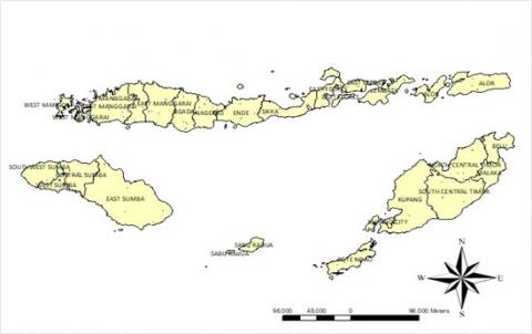
This research was conducted in the province of East Nusa Tenggara, Indonesia. The data used in this study is secondary data obtained from the BPS-Statistics Indonesia, related to the participation rate of junior high schools along with the variables that are suspected to affect it in 22 districts/cities in NTT.
The variables used along with the operational definition can be seen in Table 1.
Labor and institutional indicators further explain the socioeconomic dynamics that shape education outcomes. The Labor Force Participation Rate (LFPR) (X₄) measures the share of the working-age population participating in the labor market. A high LFPR may indicate economic pressure that reduces children’s school attendance, especially in poorer households [19]. Lastly, the number of teachers (X₅) captures the availability of teaching personnel relative to the population, reflecting the human resource capacity of the education system. Teacher availability is consistently linked to improved access, learning quality, and school participation, particularly in remote and low-come regions [21, 59].
Table 1. Variables and operational definitions
|
Variable |
Notation |
Description |
|
Junior High School Participation Rate |
Y |
Refers to the proportion of children of junior high school age who are enrolled in school across districts/cities in East Nusa Tenggara. |
|
Poverty Level |
X₁ |
Indicates the percentage of people living below the poverty line, which may limit households’ ability to support children’s education. |
|
GDP per Capita |
X₂ |
Reflects the economic condition of a region and the general welfare of its population, influencing the capacity to invest in education. |
|
Special Allocation Fund (DAK) |
X₃ |
Represents government transfers allocated to support regional infrastructure and improve education services. |
|
Labor Force Participation Rate (LFPR) |
X₄ |
Shows the share of the working-age population engaged in the labor market, which can signal economic pressures affecting school participation. |
|
Number of Teachers |
X₅ |
Describes the availability of teachers relative to the population, indicating the capacity of the education system to provide adequate services. |
4.1 Result
By using data on school participation rates in 2023 along with factors that are suspected to affect it in 22 districts/cities in NTT province, the distribution can be formed on a digital map. Figure 2 illustrates the distribution of APS in 22 districts/cities. The darker the color gradation, the higher the APS in the district/city, and viceversa.
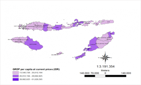
Based on Figure 3, the distribution of the variables used in this study can be classified into three, namely low, medium, and high which can be seen in Table 2.
Figure 2. Digital map of East Nusa Tenggara (NTT) Province
Figure 3. Digital map of East Nusa Tenggara (NTT) Province
Table 2. Classification of district/city distribution by low, medium, and high categories
|
Variabel |
Classification |
||
|
Low |
Medium |
High |
|
|
Gross Enrollment Rate |
Nagekeo, Sikka, East Flores, Southwest Sumba, East Sumba, South Central Timor, Belu |
Manggarai, Ngada, Lembata, Alor, Sumba Tengah, Rote Ndao, Timor Tengah Utara, Kota Kupang |
West Manggarai, East Manggarai, Ende, West Sumba, Sabu Raijua, Kupang Regency, Malacca |
|
Poverty level |
Ngada, Nagekeo, Sikka, East Flores, Kupang City, Malacca, Belu |
West Manggarai, Manggarai, Ende, Alor, Kupang Regency, North Central Timor |
East Manggarai, Lembata, Southwest Sumba, Central Sumba, West Sumba, East Sumba, Sabu Raijua, Rote Ndao, South Central Timor |
|
GDP per capita at current prices |
West Manggarai, Manggarai, East Manggarai, Nagekeo, Sikka, Lembata, Alor, Southwest Sumba, Central Sumba, West Sumba, Sabu Raijua, North Central Timor, South Central Timor, Malacca. |
Ngada, Ende, East Flores, East Sumba, Rote Ndao, Kupang Regency, Belu |
Kupang City |
|
Special Allocation Fund |
Ngada, Nagekeo, Lembata, West Sumba, Sabu Raijua, Kupang City, Malacca |
Manggarai, Ende, Sikka, East Flores, Alor, Southwest Sumba, Central Sumba, Rote Ndao, Belu |
West Manggarai, East Manggarai, East Sumba, Kupang Regency, North Central Timor, South Central Timor |
|
Labor force participation rate |
West Manggarai, Rote Ndao, Kupang City, Belu |
Ngada, Nagekeo, Ende, Sikka, East Flores, Lembata, Sabu Raijua, Kupang Regency, North Central Timor, Malacca |
Manggarai, East Manggarai, Alor, Southwest Sumba, Central Sumba, East Sumba, West Sumba, South Central Timor |
|
Teacher ratio |
Manggarai, Ngada, Nagekeo, Ende, Sikka, East Flores, West Sumba, East Sumba, Kupang City, Kupang Regency, Belu |
|
West Manggarai, East Manggarai, Lembata, Alor, Southwest Sumba, Central Sumba, Sabu Raijua, Rote Ndao, South Central Timor, North Central Timor, Malacca |
Table 3 shows that the school participation rate in the Province of NTT ranges from 73.95% to 105.68%. The poverty rate ranges from 8.61% to 31.78%. GDP per capita varies between IDR 13,549,728 and IDR 61,029,595. The Special Allocation Fund ranges from IDR 93,054,808 to IDR 327,347,244. The labor force participation rate ranges from 64.75% to 83.13%, while the teacher ratio varies from 2.62% to 6.50%.
Linear regression analysis to see the magnitude of the influence of each predictor variable on its response. The output of this analysis can be presented in Table 4.
Table 3. Statistics on the gross number of junior high school registrations in East Nusa Tenggara Province
|
Statistics |
Total Gross Registrations (%) |
Chemicals (%) |
GDP per Capita at Current Prices (IDR) |
Special Allocation Funds (Thousands of IDR) |
Labor Force Participation (%) |
Number of Teachers (%) |
|
Minimum |
73.95 |
8.61 |
13549728 |
93054808 |
64.75 |
2.629 |
|
1st Quartile |
83.80 |
14.33 |
16161222 |
136994490 |
73.70 |
4.266 |
|
Median |
91.75 |
21.82 |
18097432 |
183637333 |
76.50 |
4.692 |
|
Mean |
91.18 |
20.64 |
21231480 |
186114868 |
75.88 |
4.750 |
|
3rd Quartile |
99.33 |
26.58 |
23897736 |
226258704 |
79.06 |
5.305 |
|
Maximum |
105.68 |
31.78 |
61029595 |
327347244 |
83.13 |
6.540 |
Table 4. Output of the Ordinary Smallest Squared Regression (OLS)
|
Variabel |
Coefficient |
Stderror |
Probability |
VIF |
|
Intercept |
124.356701 |
57.404540 |
0.045728 |
-------- |
|
Poverty rate (%) |
-0.287761 |
0.411526 |
0.0494433* |
1.573266 |
|
GDP per capita at current prices (IDR) |
0.000000 |
0.000000 |
0.0907714 |
2.543247 |
|
Special allocation funds (thousands of Rp) |
0.749023 |
0.587301 |
0.037797* |
1.051172 |
|
Labor force participation (%) |
-0.697495 |
0.691779 |
0.0328333* |
2.031529 |
|
Percentage of teachers |
3.425514 |
3.973090 |
0.0401326* |
2.107488 |
VIF = Variance Inflation Factor
Based on Table 4, it can be seen that there is a negative relationship between the poverty level and the participation rate at the junior high school level, which means that every 1% increase in the poverty rate tends to decrease by 0.2878%. The effect of poverty is significant at the level of 5%. On the other hand, GDP per capita does not have a significant effect on junior high school APS. The special allocation fund has a significant effect and has a positive relationship with the APS SMP which means that every 1% increase in the special allocation fund will increase the APS SMP by 0.749%. Furthermore, there is a negative relationship between the labor force participation rate and the junior high school APS which means that every 1% increase in the labor force participation rate decreases by 0.697%. Finally, the percentage of teachers has a significant effect and has a positive relationship at the level of 5%. This means that for every 1% increase in the teacher ratio, the junior high school APS will also increase by 3.4%.
Beyond the statistical significance of individual coefficients, a critical methodological concern in the OLS specification is the potential presence of multicollinearity among the independent variables. As reported in Table 4, the Variance Inflation Factor (VIF) values range between 1.05 and 2.54, well below the conventional threshold of 10 and even beneath the more conservative benchmark of 5. From a purely diagnostic perspective, this indicates that variance inflation due to linear interdependence among predictors is minimal.
However, the interpretation of multicollinearity in this context cannot remain purely procedural. Variables such as poverty rate, GDP per capita, and labor force participation are structurally embedded within the same regional economic ecosystem and are theoretically predisposed to correlation. The relatively low VIF values therefore carry substantive implications: they suggest that each variable captures a distinct dimension of regional socioeconomic structure rather than reflecting redundant manifestations of the same underlying construct.
In other words, the stability of the estimated coefficients is not merely a statistical convenience but an indication that the model specification preserves conceptual differentiation across explanatory factors. This structural independence strengthens the internal validity of the regression results and provides a robust foundation for subsequent spatial modeling. The absence of problematic multicollinearity ensures that any detected spatial dependence in later specifications can be interpreted as genuinely spatial in nature, rather than an artifact of hidden linear relationships among predictors.
Next, it will be seen whether there is a spatial autocorrelation between districts/cities in relation to the variables studied. In this study, a spatial weighter of KNN with k = 2 was used because the researcher wanted to determine the influence of the region on the APS of junior high school based on the distance between regions. The use of a spatial weighting matrix with distance calculation in districts/cities in NTT Province because it can accommodate districts that do not directly intersect with other areas such as Rote Ndao, Sabu Raijua, Lembata, and Alor. An illustration of the KNN weighter can be seen in Figure 4.
Figure 4. The use of k-nearest neighbor (KNN) weights on the East Nusa Tenggara (NTT) provincial map
Meanwhile, visual indication of spatial dependency between regions in NTT. Statistically, it can be seen in Table 5.
Table 5. Results of Moran's I test with k-nearest neighbor (KNN) weights on $\alpha=0.10$
|
Variabel |
Moran's Value I |
Probability |
Significance |
|
Y |
-0,48404 |
0.07617* |
Significant |
|
$X_1$ |
0.29152288 |
0.03842* |
Significant |
|
$X_2$ |
0.15848030 |
0.1411 |
Insignificant |
|
$X_3$ |
-0.03920524 |
0.4825 |
Insignificant |
|
$X_4$ |
-0.24425680 |
0.4992 |
Insignificant |
|
$X_5$ |
0.047723927 |
0.06391* |
Significant |
*) Significant on $\alpha=10 \%$
The value of the Moran index is -0.48404 with a probability value of 0.07617 which is smaller than $\alpha=0.10$. This means that there is a significant negative spatial autocorrelation at the global level for junior high school level APS in the NTT region. Negative spatial autocorrelation suggests that regions with high APS tend to be close to regions with low APS. In addition, the independent variables were also significant in the spatial autocorrelation of the poverty level (and the number of teachers (with the probability of 0.038 and 0.063 respectively being smaller than $\left.\left.X_1\right) X_5\right) \alpha$. This significant value of the Moran index indicates that there are spatial patterns that need to be further analyzed. This means that the value of significant variables in 22 districts/cities in NTT is influenced by the value of the same variable in the nearest location.
Using the KNN weighter, in Figure 5 it can be seen that West Manggarai, Manggarai, East Manggarai, Ngada, and Kupang City are included in the High-High category which means that the APS of Junior High in this area is high and also adjacent to the high APS area. Meanwhile, Ende, West Sumba, Lembata, Sabu Raijua, Kupang Regency, and Malaka are included in the High-Low category. This means that the APS in these areas is high, but the adjacent areas have low APS. Furthermore, nagekeo, southwest Sumba, rote ndao, TTS, and belu can be classified as Low-High areas which means that the APS in these areas is low but adjacent to areas with high APS. In addition, Sikka, East Flores, Alor, and TTU are areas with the Low-Low category. This means that the APS in this area is low, as well as the adjacent areas have low APS as well.
Figure 5. Moran Scatterplot k-nearest neighbor (KNN) weighter
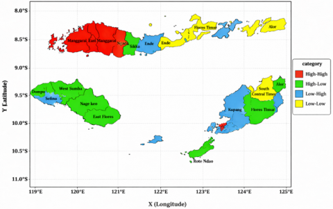
Figure 6. Map of the distribution of first-level school participation rates in East Nusa Tenggara (NTT) with k-nearest Neighbor (KNN) weights
Figure 6 illustrates the spatial clustering pattern of junior high school participation rates in NTT using the LISA based on the KNN weighting approach. The map visually distinguishes four categories of spatial association High-High, Low-Low, High-Low, and Low-High which represent the degree and direction of local spatial dependence among districts. Districts shaded in red (High-High) indicate areas with high participation rates surrounded by other high-performing neighbors, while those in green (Low-Low) denote areas where low participation rates cluster with similarly low-performing regions. Yellow areas (High-Low) and blue areas (Low-High) represent spatial outliers, suggesting districts whose educational performance differs significantly from their neighboring spatial context. The overall spatial pattern clearly exhibits positive spatial dependence, reflecting that school participation rates are not randomly distributed but geographically correlated, meaning that the educational condition in one district is influenced by the neighboring districts' performance.
Spatially, the High-High clusters are concentrated in the western and central parts of Flores Island, particularly in Manggarai, West Manggarai, and East Manggarai Regencies, as well as in Kupang City on Timor Island. These regions demonstrate localized success in education access and participation, which may be attributed to relatively better school infrastructure, teacher distribution, and higher socioeconomic welfare compared to other areas. In contrast, the Low-Low clusters appear dominantly in Sumba Island and parts of Belu, Malaka, and Alor Regencies, where limited transportation networks, low population density, and poverty constrain educational participation. The clustering of low participation rates in these regions indicates that spatial poverty traps may exist—where structural disadvantages are geographically concentrated, reinforcing the difficulty for these areas to catch up. Meanwhile, High-Low and Low-High clusters, identified in areas such as Ende, Lembata, and parts of North Central Timor, highlight spatial anomalies where local conditions differ from surrounding contexts. These mixed patterns suggest that some districts have begun to improve due to localized interventions or urban concentration, but the benefits have not yet diffused to neighboring areas.
The spatial configuration revealed by Figure 6 supports the results of the global Moran’s I statistic, which indicates significant positive spatial autocorrelation across NTT, confirming that school participation rates are spatially dependent. This finding aligns with the SEM results, which identified the presence of spatially correlated residuals—implying that unobserved regional characteristics such as geography, infrastructure, or social capital contribute to inter-district educational inequality. The map visualization thus reinforces the quantitative model findings, showing that educational accessibility in NTT is shaped not only by socioeconomic factors but also by spatial interconnectivity and geographic fragmentation. The existence of concentrated high and low participation clusters underscores the need for spatially differentiated education policies, particularly targeted interventions in Low-Low areas. Improving school accessibility, teacher mobility, and inter-island infrastructure could mitigate spatial barriers and promote educational equity across the province’s geographically fragmented districts.
Based on Table 6, by looking at the value of local spatial autocorrelation through LISA (Local Indicators of Spatial Association), it can be shown that Manggarai district is the only district that experiences spatial autocorrelation. This indicates a positive spatial grouping in the region, where the district plays a role as an area with a good junior high school APS in NTT. An illustration of the significance of this region can be clearly shown on the significance map in Figure 7.

Figure 7. Map of significance of k-nearest neighbor (KNN) weights
Furthermore, we will see spatial autocorrelation with different weights, namely the Gaussian kernel function with bandwith = 2. Based on Table 7, it can be seen that the value of the Moran index indicates a positive spatial autocorrelation. This is amplified by the probability value = 0.003779 less than $\alpha=0.05$.
Table 6. Local Indicator of Spatial Autocorrelation (LISA) value and $Z\left(L_i\right)$ with k-nearest neighbor (KNN) weighting $\alpha=0.10$
|
ID |
Territory |
$L_i$ |
$Z\left(L_i\right)$ |
Probability |
Significance |
|
1 |
Alor |
0.06732825 |
0.5468170 |
0.58450448 |
Insignificant |
|
2 |
Belu |
-0.31390811 |
-0.2820677 |
0.77789162 |
Insignificant |
|
3 |
Ende |
-0.88034807 |
-1.2446880 |
0.21324646 |
Insignificant |
|
4 |
East Flores |
0.28484294 |
0.4239043 |
0.67163564 |
Insignificant |
|
5 |
Kupang City |
0.26224625 |
1.0017442 |
0.31646717 |
Insignificant |
|
6 |
Kupang |
-0.98089604 |
-0.8318514 |
0.40549285 |
Insignificant |
|
7 |
Lembata |
-0.35428129 |
-0.9830728 |
0.32557160 |
Insignificant |
|
8 |
Malaka |
-0.71730897 |
-1.1161913 |
0.26434025 |
Insignificant |
|
9 |
Manggarai |
0.59452287 |
1.8597229 |
0.06292475* |
Significant |
|
10 |
West Manggarai |
1.05389271 |
1.4953879 |
0.13481324 |
Insignificant |
|
11 |
East Manggarai |
0.56716105 |
0.6786306 |
0.49737197 |
Insignificant |
|
12 |
Nagekeo |
-0.54504329 |
-0.8608981 |
0.38929419 |
Insignificant |
|
13 |
Ngada |
0.09464961 |
0.4667585 |
0.64067268 |
Insignificant |
|
14 |
Rote Ndao |
-0.18987108 |
-1.3695948 |
0.17081343 |
Insignificant |
|
15 |
Sabu Raijua |
-1.15697448 |
-1.4258711 |
0.15390556 |
Insignificant |
|
16 |
Sikka |
0.13064184 |
0.2643778 |
0.79148880 |
Insignificant |
|
17 |
West Sumba |
-0.47453725 |
-0.7189170 |
0.47219209 |
Insignificant |
|
18 |
Southwest Sumba |
-0.13458509 |
-0.2637811 |
0.79194862 |
Insignificant |
|
19 |
Central Sumba |
-0.05664762 |
-0.1483459 |
0.88206983 |
Insignificant |
|
20 |
East Sumba |
-0.39899827 |
-0.1947879 |
0.84555902 |
Insignificant |
|
21 |
South Central Timor |
-0.97102630 |
-0.7834111 |
0.43338576 |
Insignificant |
|
22 |
North Central Timor |
0.07007258 |
0.2889436 |
0.77262455 |
Insignificant |
* Significant on $\alpha=10\%$
Table 7. The results of Moran's I test with the weighting of the Gaussian kernel function on $\alpha=0.05$
|
Variables |
Moran's Value I |
Probability |
Conclusion |
|
Y |
0.32156126 |
0.003779 |
Significant |
|
$X_1$ |
0.48727434 |
5.437e-05 |
Significant |
|
$X_2$ |
0.44932941 |
0.0001618 |
Significant |
|
$X_3$ |
0.35676447 |
0.001717 |
Significant |
|
$X_4$ |
0.44231156 |
0.0001964 |
Significant |
|
$X_5$ |
0.35975265 |
0.001602 |
Significant |
|
Error |
0.39595653 |
0.0006649 |
Significant |
* Significant at $\alpha=5\%$ Z0.025 = 1.96, t0.95;5 = 2.570
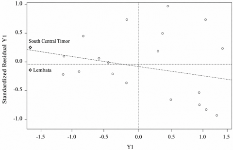
Through this weighting, the five significant free variables have spatial effects in them. Based on the hypothesis, this can be interpreted that there is a strong spatial autocorrelation. Furthermore, to see the type of relationship between adjacent areas, you can look at the Moran Scatterplot as shown in Figure 8.

Figure 8. Moran Scatterplot for Gaussian kernel function weighter
Figure 8 presents the Moran Scatterplot of junior high school participation rates (APS) using the KNN weighting scheme, and it reveals that the spatial distribution of participation across districts in East Nusa Tenggara is systematically structured rather than randomly dispersed. The positive slope of the regression line confirms the presence of global spatial dependence, indicating that participation levels in one district are statistically associated with those in neighboring districts. APS, therefore, operates within a relational spatial field rather than as an isolated administrative outcome.
The predominance of districts in Quadrant III (Low–Low) carries significant structural implications. This configuration indicates that low participation rates are geographically clustered, forming contiguous zones of disadvantage. Such clustering suggests more than localized educational underperformance; it reflects territorially embedded structural constraints. Districts with limited infrastructure, constrained fiscal capacity, and fragile institutional reach are not isolated anomalies but are spatially surrounded by similarly constrained territories. This spatial proximity reinforces cumulative disadvantage, creating what may be interpreted as a geographically reproduced inequality regime. In these areas, educational deprivation is not episodic—it is spatially sedimented.
In contrast, the High–High cluster—comprising West Manggarai, Manggarai, East Manggarai, Ngada, Kupang City, and Kupang Regency—represents spatial consolidation of educational advantage. These districts exhibit high APS values and are embedded within spatial environments characterized by similar performance. Such clustering reflects concentrated institutional capacity, relatively stronger infrastructure, and more stable teacher allocation systems. Educational performance in these regions appears to benefit from spatial reinforcement, where administrative stability and resource availability accumulate geographically rather than diffuse evenly across the province.
The High–Low configuration (e.g., West Sumba, Lembata, and Malaka) introduces a more nuanced spatial dynamic. These districts demonstrate relatively high participation despite being surrounded by lower-performing areas. This pattern may indicate localized governance effectiveness or targeted fiscal interventions that have produced internal improvements without generating spillover effects. In spatial terms, these districts function as performance enclaves rather than diffusion nodes, suggesting that proximity alone does not guarantee regional convergence.
Conversely, the Low–High districts—such as Nagekeo and Rote Ndao—illustrate the limits of geographic adjacency. Despite being positioned near higher-performing neighbors, their participation rates remain comparatively low. This pattern underscores that spatial interaction in NTT is mediated by structural filters, including maritime discontinuity, transport irregularity, fiscal absorption capacity, and administrative reach. Geographic closeness, therefore, does not automatically translate into developmental spillover. Spatial dependence in archipelagic regions operates within infrastructural and institutional constraints.
What renders Figure 8 analytically decisive is the asymmetry of its spatial configurations. Advantage and disadvantage do not distribute evenly, nor do they follow a uniform diffusion logic. Some districts accumulate institutional strength, others remain embedded in spatial traps, and a few occupy transitional positions. This heterogeneity directly challenges the independence assumption underlying conventional OLS regression and substantiates the necessity of spatial econometric modeling.
Figure 8 thus provides empirical evidence that junior high school participation in East Nusa Tenggara is embedded within a differentiated socio-spatial architecture. Educational outcomes are co-produced through geographic proximity, institutional capacity, and infrastructural accessibility. The scatterplot does not merely categorize districts into quadrants; it exposes the structural geography of educational inequality—where space is not a backdrop, but an active determinant shaping the distribution of opportunity.
The spatial distribution of junior high school participation rates across the 22 districts of NTT Province using the Gaussian Kernel weighting function. Unlike the KNN approach, which defines spatial proximity based on a fixed number of neighbors, the Gaussian Kernel model applies a continuous distance-based weighting scheme that accounts for the gradual decline in spatial influence with increasing distance. The map identifies four local spatial association categories—High-High, Low-Low, High-Low, and Low-High—representing the intensity and direction of spatial autocorrelation. The High-High clusters (red regions) indicate districts with high school participation surrounded by similarly high-performing areas, while the Low-Low clusters (green regions) denote areas of consistently low participation. High-Low (yellow) and Low-High (blue) clusters reflect spatial outliers that deviate from neighboring patterns, highlighting regions undergoing transition or affected by unique local factors.
The spatial pattern observed in Figure 9 reveals a clear east–west divide in educational participation across NTT. The High-High clusters are primarily located in Manggarai, West Manggarai, East Manggarai, and East Sumba, which are relatively more developed districts with better infrastructure. These areas exhibit strong positive spatial association, implying that educational attainment tends to cluster in more urbanized and economically active regions. Conversely, Low-Low clusters appear in Sumba Barat Daya, Central Sumba, and parts of Belu, suggesting that low participation rates persist within geographically isolated and socioeconomically constrained districts. These patterns indicate that the Gaussian kernel function successfully captures spatial diffusion effects, where the influence of distance is continuous and multidirectional, revealing more nuanced relationships than the discrete KNN model. The High-Low and Low-High outlier zones, such as Kupang Regency and Ngada, represent transitional regions where educational performance differs significantly from surrounding areas, possibly due to policy interventions or differential school resource allocation.
Overall, the spatial configuration displayed in Figure 9 reinforces the findings from the SEM, which confirmed significant spatial dependence across districts. The concentration of High-High and Low-Low clusters supports the presence of localized inequality and spatial clustering in educational outcomes, consistent with the positive Moran’s I statistic obtained using the Gaussian kernel weighting. However, the presence of spatial outliers also reveals the heterogeneity of educational development within the province, underscoring the role of geographical distance and infrastructure disparities in shaping participation levels. This visualization thus highlights the necessity for spatially adaptive education policies that consider not only district-level socioeconomic factors but also the continuous spatial interactions between regions, particularly in an archipelagic context where physical connectivity directly affects educational access and quality.
This study provides robust empirical evidence of spatial dependence in junior high school participation rates across districts in NTT, Indonesia. The results of the SEM demonstrate that poverty exerts a significant negative effect on participation—where a 1% increase in poverty reduces the participation rate by approximately 0.59%—while teacher availability exerts a positive influence, with every 1% increase associated with a 0.93% improvement in participation. The model’s explanatory power (R² = 0.332) suggests that nearly one-third of participation variability can be explained by spatial and socioeconomic factors. Diagnostic tests, including the Moran’s Index (-0.48404; p = 0.07617) and the LM statistics, confirm the existence of both global and local spatial autocorrelation, validating the application of the SEM as the most appropriate model based on its lowest AIC value. The identification of High-High clusters in Manggarai and Low-Low clusters in Sumba and Belu further underscores the spatial concentration of educational inequality within the province.
Beyond statistical confirmation, these spatial patterns have profound policy implications. The existence of spatial clusters indicates that educational inequality in NTT is not randomly distributed but structurally embedded in the geography of the province. This finding calls for spatially targeted and regionally coordinated education policies rather than uniform national programs. Districts identified as Low-Low clusters should be prioritized for teacher redistribution schemes, poverty alleviation efforts, and infrastructure development—particularly in remote and island areas where physical accessibility remains a barrier to schooling. Conversely, High-High clusters such as Manggarai can serve as regional learning hubs, facilitating knowledge transfer and mentorship to neighboring districts. Moreover, integrating education planning with transport, communication, and digital infrastructure is essential to ensure that spatial connectivity translates into equitable educational access. These insights highlight the necessity for a multi-sectoral, spatially informed approach to achieving Sustainable Development Goal 4 (Quality Education) in archipelagic regions.
Methodological reflections and future research directions further extend the study’s contribution. Although the SEM explains a meaningful portion of spatial variation, the moderate R² (0.332) indicates that other unobserved factors—such as infrastructure quality, inter-island transport connectivity, school accessibility, and digital inclusion—may also drive disparities. The analysis, limited to cross-sectional data from 2023, cannot capture temporal changes or policy impacts over time. Future studies should therefore adopt spatial panel models to explore longitudinal dynamics and compare the persistence of spatial effects. Additionally, testing alternative spatial weighting structures—such as Queen, Rook, or adaptive distance-based kernels—would enhance model robustness and comparability. Expanding the analytical framework to include qualitative and institutional dimensions, such as governance effectiveness, community engagement, and local cultural attitudes toward education, could provide deeper insight into the spatial mechanisms of inequality.
This study advances both empirical understanding and methodological practice in spatial education research. It establishes that educational participation in island regions like NTT is shaped not only by socioeconomic variables but also by spatial interdependencies across districts. Addressing these inequalities requires policies that recognize the geographic logic of education—policies that are data-driven, spatially adaptive, and socially inclusive. By integrating spatial econometrics with education policy design, this research contributes to a more grounded, regionally responsive framework for promoting equitable education in Indonesia’s archipelagic context and beyond.
[1] Azzahra, A., Rahayu, R., Marlina, N.S., Saebah, N., Saputro, W.E. (2024). The role of education in economic growth and breaking the chain of poverty in Indonesia. Journal of Management, Economic, and Financial, 2(2): 55-63.
[2] Urata, S., Kuroda, K., Tonegawa, Y. (2023). Sustainable Development Disciplines for Humanity: Breaking Down the 5Ps—People, Planet, Prosperity, Peace, and Partnerships (p. 187). Springer Nature. https://doi.org/10.1007/978-981-19-4859-6
[3] van Niekerk, A.J. (2025). The New Global Economy and Economic Inclusion: Achieving the SDGs Together. In West to East: A New Global Economy in the Making? Achieving the SDGs, pp. 163-213. https://doi.org/10.1007/978-3-031-93267-0_5
[4] Sulashvili, N., Khusseyn, V., Hussin, D., Gabunia, L., et al. (2025). Perspectives on English language acquisition, role and its impact in enhancing on education mobility, socio-cultural, institutional integration and medical labor market integration in Europe and worldwide in the context of educational globalization. Georgian Scientists, 7(4): 59-96. https://doi.org/10.52340/gs.2025.07.04.03
[5] Chen, M.K., Shih, Y.H. (2025). The role of higher education in sustainable national development: Reflections from an international perspective. Edelweiss Applied Science and Technology, 9(4): 1343-1351. https://doi.org/10.55214/25768484.v9i4.6262
[6] (BPS): B.P.S. (2024). Database Indikator Sosial dan Pendidikan 2024. BPS-Statistics Indonesia. https://www.bps.go.id/id/publication/2024/11/22/c20eb87371b77ee79ea1fa86/statistik-pendidikan-2024.html.
[7] (BPS): B.P.S. (2023). Statistik Pendidikan Indonesia 2023. BPS-Statistics Indonesia. https://www.bps.go.id/id/publication/2023/11/24/54557f7c1bd32f187f3cdab5/statistik-pendidikan-2023.html.
[8] Hakim, A. (2020). Faktor penyebab anak putus sekolah. Jurnal Pendidikan, 21(2): 122-132. https://doi.org/10.33830/jp.v21i2.907.2020
[9] Dietz, R.D. (2002). The estimation of neighborhood effects in the social sciences: An interdisciplinary approach. Social Science Research, 31(4): 539-575. https://doi.org/10.1016/s0049-089x(02)00005-4
[10] Gu, J. (2016). Spatial diffusion of social policy in China: Spatial convergence and neighborhood interaction of vocational education. Applied Spatial Analysis and Policy, 9(4): 503-527. https://doi.org/10.1007/s12061-015-9161-3
[11] Gulson, K.N., Symes, C. (2007). Knowing One's Place: Educational Theory, Policy, and the Spatial Turn. In Spatial Theories of Education, pp. 1-16. Routledge. https://doi.org/10.4324/9780203940983-7
[12] Park, Y., Rogers, G.O. (2015). Neighborhood planning theory, guidelines, and research: Can area, population, and boundary guide conceptual framing? Journal of Planning Literature, 30(1): 18-36. https://doi.org/10.1177/0885412214549422
[13] Brattbakk, I. (2014). Block, neighbourhood or district? The importance of geographical scale for area effects on educational attainment. Geografiska Annaler: Series B, Human Geography, 96(2): 109-125. https://doi.org/10.1111/geob.12040
[14] Ghosh, S. (2013). Participation in school choice: A spatial probit analysis of neighborhood influence. The Annals of Regional Science, 50(1): 295-313. https://doi.org/10.1007/s00168-011-0469-x
[15] Tang, Y., Jing, L., Li, H., Atkinson, P.M. (2016). A multiple-point spatially weighted k-NN method for object-based classification. International Journal of Applied Earth Observation and Geoinformation, 52: 263-274. https://doi.org/10.1016/j.jag.2016.06.017
[16] Kibanov, M., Becker, M., Mueller, J., Atzmueller, M., Hotho, A., Stumme, G. (2018). Adaptive KNN using expected accuracy for classification of geo-spatial data. In Proceedings of the 33rd Annual ACM Symposium on Applied Computing, pp. 857-865. https://doi.org/10.1145/3167132.3167226
[17] Ver Hoef, J.M., Temesgen, H. (2013). A comparison of the spatial linear model to nearest neighbor (k-NN) methods for forestry applications. PloS One, 8(3): e59129. https://doi.org/10.1371/journal.pone.0059129
[18] Sotiropoulou, K.F., Vavatsikos, A.P. (2023). A decision-making framework for spatial multicriteria suitability analysis using PROMETHEE II and k nearest neighbor machine learning models. Journal of Geovisualization and Spatial Analysis, 7(2): 20. https://doi.org/10.1007/s41651-023-00151-3
[19] Adejumo, O.O., Asongu, S.A., Adejumo, A.V. (2021). Education enrolment rate vs employment rate: Implications for sustainable human capital development in Nigeria. International Journal of Educational Development, 83: 102385. https://doi.org/10.1016/j.ijedudev.2021.102385
[20] Hasan, Z. (2022). The effect of human development index and net participation rate on the percentage of poor population: A case study in Riau Province, Indonesia. International Journal of Islamic Economics and Finance Studies, 8(1): 24-40. https://doi.org/10.54427/ijisef.964861
[21] Duflo, E., Dupas, P., Kremer, M. (2015). School governance, teacher incentives, and pupil–teacher ratios: Experimental evidence from Kenyan primary schools. Journal of Public Economics, 123: 92-110. https://doi.org/10.3386/w17939
[22] Labib, S.M., Huck, J.J., Lindley, S. (2021). Modelling and mapping eye-level greenness visibility exposure using multi-source data at high spatial resolutions. Science of the Total Environment, 755: 143050. https://doi.org/10.1016/j.scitotenv.2020.143050
[23] Pramoedyo, H., Ngabu, W., Riza, S., Iriany, A. (2024). Spatial analysis using geographically weighted ordinary logistic regression (GWOLR) method for prediction of particle-size fraction in soil surface. IOP Conference Series: Earth and Environmental Science, 1299(1): 012005. https://doi.org/10.1088/1755-1315/1299/1/012005
[24] Roodman, D., Nielsen, M.Ø., MacKinnon, J.G., Webb, M.D. (2019). Fast and wild: Bootstrap inference in Stata using boottest. The Stata Journal, 19(1): 4-60. https://doi.org/10.1177/1536867X19830877
[25] Gomes, M.J.T.L., Cunto, F., da Silva, A.R. (2017). Geographically weighted negative binomial regression applied to zonal level safety performance models. Accident Analysis & Prevention, 106: 254-261. https://doi.org/10.1016/j.aap.2017.06.011
[26] Anggelitha, T., Widiyanto, W., Suryanadi, J., Wulandari, A. (2025). The effect of technology-based learning on learning motivation of Buddhist Sunday school. Journal of Education, Religious, and Instructions, 3(1): 48-59. https://doi.org/10.60046/joeri.v3i1.131
[27] Nurdessyanah, A., Maryani, E., Sapriya, S. (2025). The influence of the problem-based learning model on the improvement of geography literacy skills. Journal of Innovation and Research in Primary Education, 4(3): 789-799. https://doi.org/10.56916/jirpe.v4i3.1593
[28] Jaya, I.G.N.M., Toharudin, T., Abdullah, A.S. (2018). A Bayesian spatial autoregressive model with k-NN optimization for modeling the learning outcome of the junior high schools in West Java. Model Assisted Statistics and Applications, 13(3): 207-219. https://doi.org/10.3233/mas-180435
[29] Janatabadi, F., Ermagun, A. (2024). Access weight matrix: A place and mobility infused spatial weight matrix. Geographical Analysis, 56(4): 746-767. https://doi.org/10.1111/gean.12395
[30] Purwaningsih, T., Winarko, E., Mustofa, K. (2025). Enhancing accuracy of spatiotemporal model estimation using modified binary distance spatiotemporal weight matrix. International Journal of Intelligent Engineering & Systems, 18(8): 383-397. https://doi.org/10.22266/ijies2025.0930.24
[31] Isnan, S., bin Abdullah, A.F., Shariff, A.R., Ishak, I., et al. (2025). Moran’s I and Geary’s C: Investigation of the effects of spatial weight matrices for assessing the distribution of infectious diseases. Geospatial Health, 11(s1). https://doi.org/10.4081/gh.2016.380
[32] Musdalifah, S., Hardiansyah, S. (2024). Application of the k-nearest neighbor ensemble method in predicting the human development index and its relationship with the unemployment rate in central Sulawesi Province. The Journal of Academic Science, 1(8): 979-988. https://doi.org/10.59613/w1ebc495
[33] Ru, Y., Tennant, E., Matteson, D.S., Barrett, C.B. (2026). Spatial heterogeneity in machine learning-based poverty mapping: Where do models underperform?. Geography and Sustainability, 7(2): 100413. https://doi.org/10.1016/j.geosus.2026.100413
[34] Wang, M., Gao, F., Dong, J., Li, H.C., Du, Q. (2023). Nearest neighbor-based contrastive learning for hyperspectral and LiDAR data classification. IEEE Transactions on Geoscience and Remote Sensing, 61: 1-16. https://doi.org/10.1109/tgrs.2023.3236154
[35] Sun, L., Zhang, J., Ding, W., Xu, J. (2022). Feature reduction for imbalanced data classification using similarity-based feature clustering with adaptive weighted K-nearest neighbors. Information Sciences, 593: 591-613. https://doi.org/10.1016/j.ins.2022.02.004
[36] Kubara, M., Kopczewska, K. (2024). Akaike information criterion in choosing the optimal k-nearest neighbours of the spatial weight matrix. Spatial Economic Analysis, 19(1): 73-91. https://doi.org/10.1080/17421772.2023.2176539
[37] Halder, R.K., Uddin, M.N., Uddin, M.A., Aryal, S., Khraisat, A. (2024). Enhancing K-nearest neighbor algorithm: A comprehensive review and performance analysis of modifications. Journal of Big Data, 11(1): 113. https://doi.org/10.1186/s40537-024-00973-y
[38] Zuo, W., Zhang, D., Wang, K. (2008). On kernel difference-weighted k-nearest neighbor classification. Pattern Analysis and Applications, 11(3): 247-257. https://doi.org/10.1007/s10044-007-0100-z
[39] Fan, G.F., Guo, Y.H., Zheng, J.M., Hong, W.C. (2019). Application of the weighted k-nearest neighbor algorithm for short-term load forecasting. Energies, 12(5): 916. https://doi.org/10.3390/en12050916
[40] Sohn, M.H., You, T., Lee, S.L., Lee, H. (2003). Corporate strategies, environmental forces, and performance measures: A weighting decision support system using the k-nearest neighbor technique. Expert Systems with Applications, 25(3): 279-292. https://doi.org/10.1016/s0957-4174(03)00070-8
[41] Soemartojo, S.M., Ghaisani, R.D., Siswantining, T., Shahab, M.R., Ariyanto, M.M. (2018). Parameter estimation of geographically weighted regression (GWR) model using weighted least square and its application. AIP Conference Proceedings, 2014(1): 020081. https://doi.org/10.1063/1.5054485
[42] Lai, J., Zhu, W., Cui, D., Mao, L. (2023). Extension of the GLMM. HP package to zero-inflated generalized linear mixed models and multiple regression. Journal of Plant Ecology, 16(6): rtad038. https://doi.org/10.1093/jpe/rtad038
[43] Anselin, L. (2022). Spatial Econometrics. In Handbook of Spatial Analysis in the Social Sciences, pp. 101-122. https://doi.org/10.4337/9781789903942.00014
[44] Brunsdon, C., Comber, A. (2021). Opening practice: Supporting reproducibility and critical spatial data science. Journal of Geographical Systems, 23(4): 477-496. https://doi.org/10.1007/s10109-020-00334-2
[45] Florax, R.J., Folmer, H., Rey, S.J. (2003). Specification searches in spatial econometrics: The relevance of Hendry’s methodology. Regional Science and Urban Economics, 33(5): 557-579. https://doi.org/10.1016/S0166-0462(03)00002-4
[46] Elhorst, J.P., Lacombe, D.J., Piras, G. (2012). On model specification and parameter space definitions in higher order spatial econometric models. Regional Science and Urban Economics, 42(1-2): 211-220. https://doi.org/10.1016/j.regsciurbeco.2011.09.003
[47] See, L. (2021). Web-based tools for exploratory spatial data analysis. In Handbook of Regional Science, pp. 1671-1689. https://doi.org/10.1007/978-3-662-60723-7_115
[48] Billé, A.G., Salvioni, C., Benedetti, R. (2018). Modelling spatial regimes in farms technologies. Journal of Productivity Analysis, 49(2): 173-185. https://doi.org/10.1007/s11123-018-0529-7
[49] de Baar, J.H., Garcia-Marti, I., van der Schrier, G. (2023). Spatial regression of multi-fidelity meteorological observations using a proxy-based measurement error model. Advances in Science and Research, 20: 49-53. https://doi.org/10.5194/asr-20-49-2023
[50] Jaya, C.K., Sunitha, R., Mathew, A.T. (2019). Security prediction of high voltage transmission system (HVTS) based on k-nearest neighbor (k-NN) classifier technique. Journal of Intelligent & Fuzzy Systems, 36(6): 5773-5782. https://doi.org/10.3233/jifs-181617
[51] UNESCO Institute for Statistics. (2022). Report on UIS activities in 2022. https://www.uis.unesco.org/sites/default/files/medias/fichiers/2025/08/2022_UIS_Narrative_Report.pdf.
[52] World Bank. (2025). Indonesia poverty and equity brief: October 2025 (English). http://documents.worldbank.org/curated/en/099638104212531827.
[53] Rahman, A., Sirojuzilam, S., Lubis, I., Pratomo, W.A. (2023). Income inequality between provinces in Indonesia. Jurnal Ekonomi Malaysia, 57(3): 59-74.
[54] Liu, W., Li, J., Zhao, R. (2023). The effects of rural education on poverty in China: A spatial econometric perspective. Journal of the Asia Pacific Economy, 28(1): 176-198. https://doi.org/10.1080/13547860.2021.1877240
[55] Spada, A., Fiore, M., Galati, A. (2024). The impact of education and culture on poverty reduction: Evidence from panel data of European countries. Social Indicators Research, 175(3): 927-940. https://doi.org/10.1007/s11205-023-03155-0
[56] Alnour, M., Bilgili, F., Khan, K. (2026). Spatial dimensions of energy poverty alleviation and socioeconomic sustainability in Sub-Saharan Africa. Sustainable Development. https://doi.org/10.1002/sd.70723
[57] Andhini, S., Gunawan, J., Chen, H.Y. (2023). Influence of general allocation fund, special allocation fund, and capital expenditure on financial performance of local government. International Journal of Contemporary Accounting, 5(2): 125-140. https://doi.org/10.25105/ijca.v5i2.17381
[58] Pravitasari, A.E., Rustiadi, E., Priatama, R.A., Murtadho, A., et al. (2021). Spatiotemporal distribution patterns and local driving factors of regional development in Java. ISPRS International Journal of Geo-Information, 10(12): 812. https://doi.org/10.3390/ijgi10120812
[59] Tipayalai, K., Subchavaroj, C. (2024). Assessing the spatial impact of educational attainment on poverty reduction in Thailand. Education Economics, 32(4): 538-555. https://doi.org/10.1080/09645292.2023.2244702
[60] Bayard, S., Imlig, F., Schmid, S. (2022). Socio-spatial conditions of educational participation: A typology of municipalities in the Canton of Zurich. Education Sciences, 12(2): 73. https://doi.org/10.3390/educsci12020073
[61] Seddon, T. (2014). Renewing sociology of education? Knowledge spaces, situated enactments, and sociological practice in a world on the move. European Educational Research Journal, 13(1): 9-25. https://doi.org/10.2304/eerj.2014.13.1.9
[62] Kristanto, G.A., Saiya, H., Kemala, D., Pamungkas, S. (2025). Assessing Rural Sustainability in Nangapanda, East Nusa Tenggara, Indonesia. In a Liveable Kampung: The Challenges of Urban Expansion in Greater Jakarta and East Nusa Tenggara, pp. 143-168. Singapore: Springer Nature Singapore. https://doi.org/10.1007/978-981-96-7866-2_8
[63] Kaban, P.A., Supardi, K., Kurniawan, R., Kim, Y., et al. (2024). Investigating adolescent vulnerability in Indonesia: A socio-remote sensing big data analytics study using night light data. IEEE Access, 12: 14800-14818. https://doi.org/10.1109/ACCESS.2024.3355963
[64] Tuhfah, K.S., Arifin, A.F.A., Izdhihar, M.F., Tallo, A.J. (2024). Spatial configuration based on relationship between buildings and road network in Kupang City, East Nusa Tenggara Province, Indonesia. Arteks: Jurnal Teknik Arsitektur, 9(1): 89-98. https://doi.org/10.30822/arteks.v9i1.2894
[65] Maschke, S., Wellnitz, V. (2020). The method of the socio-spatial map for the reconstruction of transformative educational processes in educational contexts. International Journal for Research on Extended Education, 7(2): 17-18. https://doi.org/10.3224/ijree.v7i2.08
[66] Widodo, B.S., Suprapto, F.A., Saginov, K., Prastiyono, H., et al. (2025). Integration of geospatial data in education management systems: A multiple study in eastern Java regions, Indonesia. Geo Journal of Tourism and Geosites, 62(4): 2240-2248. https://doi.org/10.30892/gtg.62421-1587
[67] Zhu, A.X., Turner, M. (2022). How is the third law of geography different? Annals of GIS, 28(1): 57-67. https://doi.org/10.1080/19475683.2022.2026467.
[68] Zhang, J., Zhang, K., Zhao, F. (2020). Research on the regional spatial effects of green development and environmental governance in China based on a spatial autocorrelation model. Structural Change and Economic Dynamics, 55: 1-11. https://doi.org/10.1016/j.strueco.2020.06.001
[69] Bernard, J., Keim-Klärner, S. (2023). Disadvantaged and disadvantaging regions: Opportunity structures and social disadvantage in rural peripheries. Tijdschrift Voor Economische en Sociale Geografie, 114(5): 463-478. https://doi.org/10.1111/tesg.12589
[70] Bernard, J., Steinführer, A., Klärner, A., Keim-Klärner, S. (2023). Regional opportunity structures: A research agenda to link spatial and social inequalities in rural areas. Progress in Human Geography, 47(1): 103-123. https://doi.org/10.1177/03091325221139980
[71] Davies, J., Donnelly, M. (2024). Spatial division of opportunity: Local economic context, elite trajectories, and the widening participation industry. Social & Cultural Geography, 25(6): 852-871. https://doi.org/10.1080/14649365.2023.2203119
[72] Otero, G., Carranza, R., Contreras, D. (2023). Spatial divisions of poverty and wealth: Does segregation affect educational achievement? Socio-Economic Review, 21(1): 617-641. https://doi.org/10.1093/ser/mwab022
[73] LeSage, J., Pace, R.K. (2009). Introduction to Spatial Econometrics. Chapman and Hall/CRC.
[74] Tomul, E., Savasci, H.S. (2012). Socioeconomic determinants of academic achievement. Educational Assessment, Evaluation and Accountability, 24(3): 175-187. https://doi.org/10.1007/s11092-012-9149-3
[75] Du, H., Cai, Y., Zhang, Q. (2026). Dispossessing the vulnerable or building resilience? Assessing the long-term impacts of rural land expropriation on poverty alleviation sustainability in China. Habitat International, 167: 103633. https://doi.org/10.1016/j.habitatint.2025.103633
[76] Tao, M., Lin, B., Silva, E. (2024). China's household's energy poverty mitigation: An inclusive finance perspective. Energy, 313: 134114. https://doi.org/10.1016/j.energy.2024.134114
[77] Dahan, M., Nisan, U. (2022). Late payments, liquidity constraints and the mismatch between due dates and paydays. Water Resources Research, 58(1): e2021WR030303. https://doi.org/10.1029/2021wr030303
[78] Long, T., Bu, K., Du, P., Wang, Z. (2024). Can educational investment mitigate the impact of aging on household leverage ratio? International Review of Economics & Finance, 89: 1335-1347. https://doi.org/10.1016/j.iref.2023.09.001
[79] Wood, L., Rolleri, L.A. (2014). Designing an effective sexuality education curriculum for schools: Lessons gleaned from the South (ern) African literature. Sex Education, 14(5): 525-542. https://doi.org/10.1080/14681811.2014.918540
[80] Wei, B., Mao, X., Liu, S., Liu, M., et al. (2024). Breaking the poverty trap in an ecologically fragile region through ecological engineering: A close-up look at long-term changes in ecosystem services. Journal of Environmental Management, 358: 120921. https://doi.org/10.1016/j.jenvman.2024.120921
[81] Janz, T., Augsburg, B., Gassmann, F., Nimeh, Z. (2023). Leaving no one behind: Urban poverty traps in Sub-Saharan Africa. World Development, 172: 106388. https://doi.org/10.1016/j.worlddev.2023.106388
[82] Yang, Z., Yang, D., Sun, D., Zhong, L. (2023). Ecological and social poverty traps: Complex interactions moving toward sustainable development. Sustainable Development, 31(2): 853-864. https://doi.org/10.1002/sd.2425
[83] Kawuryan, S.P., Sayuti, S.A., Dwiningrum, S.I.A. (2021). Teachers quality and educational equality achievements in Indonesia. International Journal of Instruction, 14(2): 811-830.
[84] Kingdon, G.G., Muzammil, M. (2003). The political economy of education in India: Teacher politics in Uttar Pradesh. (No Title).
[85] Hanushek, E.A., Woessmann, L. (2020). The economic impacts of learning losses.
[86] Faguet, J.P. (2014). Decentralization and governance. World Development, 53: 2-13. https://doi.org/10.1016/j.worlddev.2013.01.002
[87] Filmer, D., Fox, L. (2014). Youth Employment in Sub-Saharan Africa. World Bank Publications.
[88] Tadjoeddin, M.Z., Yumna, A., Gultom, S.E., Rakhmadi, M.F., Suryahadi, A. (2021). Inequality and violent conflict: New evidence from selected provinces in Post-Soeharto Indonesia. Journal of the Asia Pacific Economy, 26(3): 552-573. https://doi.org/10.1080/13547860.2020.1773607
[89] Widyastaman, P.A., Hartono, D. (2024). Geographic distribution of economic inequality and crime in Indonesia: Exploratory spatial data analysis and spatial econometrics approach. Applied Spatial Analysis and Policy, 17(2): 547-571. https://doi.org/10.1007/s12061-023-09556-5
[90] Lee, K.S., Eom, J.K. (2025). Spatiotemporal dynamics of visitors to Jeju Island: Hotspot and spatial autocorrelation analyses using mobile phone data. PLoS One, 20(4): e0321694. https://doi.org/10.1371/journal.pone.0321694
[91] Song, Y., Cibin, A. (2024). Optimizing spatial weight matrices in spatial econometrics: A graph-theoretic approach based on shortest path algorithms. International Review for Spatial Planning and Sustainable Development, 12(2): 181-200. https://doi.org/10.14246/irspsd.12.2_181
[92] Rüttenauer, T. (2022). Spatial regression models: A systematic comparison of different model specifications using Monte Carlo experiments. Sociological Methods & Research, 51(2): 728-759. https://doi.org/10.1177/0049124119882467
[93] Pallikonda, A.K., Bandarapalli, V.K., Vipparla, A. (2025). Real-time anomaly detection in IoT networks using a hybrid deep learning model. Acadlore Transactions on AI and Machine Learning, 4(4): 235-246. https://doi.org/10.56578/ataiml040401
[94] Mandave, D.D., Patil, L.V. (2025). A Statistically rigorous comparison of MobileNetV2 and EfficientNet-B0 for facial expression recognition on the FER2013 benchmark. Information Dynamics and Applications, 4(4): 189-200. https://doi.org/10.56578/ida040401