Ramisetti Uma Maheswari*![]() | J. Avanija
| J. Avanija![]()
© 2026 The authors. This article is published by IIETA and is licensed under the CC BY 4.0 license (http://creativecommons.org/licenses/by/4.0/).
OPEN ACCESS
Remote sensing imagery has become an essential data source for large-scale urban monitoring, transportation analysis, and military surveillance. However, accurate vehicle type detection in high-resolution aerial images remains challenging due to small object size, complex backgrounds, and significant variations in object orientation and scale. To address these issues, this study proposes a hybrid deep learning framework that integrates geometric data augmentation with a Densely Connected Transformer-in-Transformer (Dense-TNT) architecture. The proposed approach combines the strong local feature extraction capability of DenseNet with the global contextual modeling ability of Transformer-in-Transformer modules, enabling more effective representation of both fine-grained spatial details and long-range dependencies. In addition, geometric augmentation strategies, including rotation, scaling, flipping, and translation, are employed to improve model robustness against orientation and scale variations in aerial imagery. Experiments conducted on two benchmark datasets, VEDAI and ISPRS Potsdam, demonstrate that the proposed Dense-TNT framework consistently outperforms several representative methods, including Faster-RCNN, YOLOv3, AGMFNet, and TMAFNet. The model achieves an overall accuracy of 88.99% on the VEDAI dataset and 89.51% on the ISPRS Potsdam dataset, indicating its effectiveness for vehicle type detection in complex remote sensing scenarios. These results confirm that the integration of geometric augmentation and hybrid convolution-transformer architectures provides a robust solution for small object detection in high-resolution aerial imagery.
remote sensing imagery, vehicle type detection, geometric augmentation, DenseNet, transformer-in-transformer, hybrid CNN–transformer network, small object detection
Bounding box is used to create region of interest in the input images which can be used for target detection [1, 2]. Remote sensing (RS) is classified into three classes based on changed imaging bands: 1) optical RS, 2) synthetic aperture radar (SAR), and 3) infrared RS, amongst others. The target identification process in optical RSIs is required for various applications, such as identifying geological hazards, urban planning, mapping land-use environmental monitoring, updating Geographic Information Systems (GIS), and precision farming. Vehicle type recognition in aerial images is needed for critical applications such as military and civilians. The approach mentioned by authors is used for traffic control and military target attacks [3].
This approach provides valuable support for applications such as real-time vehicle data collection, accident monitoring, and addressing illegal parking [4]. Aerial vehicle type identification enables the collection of substantial combat information in military contexts [5]. Different methods for vehicle identification from aerial images have been advancing recently with improved efficiency. Authors implemented the filter to every possible location within the image using the sliding-window method, which is among the commonly employed techniques [6]. Initially, manually crafted features and shallow learning-related characteristics constrained the ability to effectively represent and extract features. Sliding-window approach led to repetitive calculations, thereby increasing processing burden associated with results. Numerous researchers have introduced recent innovations in computer vision aimed at greatly enhancing the object detection process in remote sensing imagery. However, object recognition techniques developed for typical images cannot be directly utilized on aerial images. This happens due to issues such as varying object sizes, degraded images, arbitrary orientations and inconsistent object intensities [7, 8].
The Dense-TNT model uses Geometric Augmentations to help identify different types of vehicles in remote sensing images. It combines strong data enhancement methods with a mixed design that includes convolutional layers and transformers. The proposed approach uses Transformer-in-Transformer (TNT) blocks for better modeling of features. The use of dense convolution layers helps in local feature extraction. By utilizing these techniques, the accurate detection of vehicle types is possible by overcoming the challenges faced, easing the task of remote sensing.
1.1 Motivation of the research
In complex scenarios for better detection of vehicle types for transportation and urban planning the need for remote sensing data becomes very important. The issues that arise during this process include the variation in image size, orientation and occlusion. Most of the traditional method encounters his problem. Considering this issue the Dense-TNT framework combining geometric augmentation has been proposed. In order to capture the features properly. The proposed approach utilizes the transformers, convolution layers and dense net. The robustness of the proposed method was improved applying Geometric augmentation to the images.
During vehicle detection process in remote sensing images, the visibility of object is affected due to the variation in resolution and image orientation. High vehicle type likeness, along with shadows, occlusions, and dense urban backgrounds, often results in inaccurate diagnosis. Limited annotated datasets and processing requirements further limit model performance. To detect vehicle categories accurately and robustly, complex architectures combining geometric augmentations and convolutional-transformer features are required.
1.2 Main contribution of our work
· To develop an innovative structure combining geometric augmentations with the Dense-TNT architecture to increase vehicle type organization in aerial imagery. By integrating geometric augmentations (rotations, scaling, flipping, and translations), the methodology improves model robustness to orientation and scale variations.
· The Dense-TNT model synergizes DenseNet's local feature extraction capabilities with the Transformer-in-Transformer's global spatial dependency learning, ensuring better performance in detecting diverse vehicle types.
· Experimental results on benchmark datasets highlight its accuracy, precision, and scalability, making it a practical solution for remote sensing vehicle detection tasks.
The rest of the content of this research is organized as follows: Section 2 focuses on the background analysis of vehicle type diagnosis utilizing RS images. Section 3 provides a complete overview of our suggested technique. In Section 4, we discuss the experimental results obtained from two different datasets. Section 5 focuses on the conclusion and future work.
Transformer and deep learning models were used to improve the efficiency of vehicle detection in remote sensing images. These methods have benefits in providing better accuracy and efficiency, but have limitations such as scalability and working with diversified datasets. Considering these limitations, the authors [9] used vision transformer architectures combined with multihead attention in order to model spatial relationships. The accuracy of this model is around 97.5% and also the model maintains around 96% accuracy with the compressed version. The increase in accuracy is due to the use of transformer architecture to capture the dependencies in long-range. The model’s limitation is high computation cost on training large scale data.
The authors [10] proposed deep learning architecture combining segmentation and attention to handle variations in unlabelled dataset. Also, this framework uses data from various sources which increases the complexity of the model. The deep learning architectures with deep residual network combining sealion optimization method was proposed [11]. The UAV based detection of vehicle monitoring was proposed. The deep learning architecture used was hybrid YOLO and GhoshNet [12]. The accuracy of the model was better and efficient for vehicle type detection.
The UAV image detection process involves using satellite dataset with high resolution. The use of 3 dimensional feature maps integrated with YOLOv3 architecture. This approach improves accuracy considering the spatial-depth features. The accuracy of the model is about 94% [13]. Lightweight convolution model based on the YOLOv4 architecture was used to detect small objects in aerial images. Also, the computational cost of this model was low. These advantages were achieved by using conditional diffusion process and conditional variational Autoencoder. The model can handle irregularities with better accuracy and computational efficiency handling diversified dataset [14, 15].
2.1 Research gap
The traditional methods will not capture global relationships, but the transformer models work accurately even with low resolution images. Also, the availability of dataset is limited and the inputs are noisy and low quality. These issues should be addressed to work with real time applications. The framework proposed should handle diversified dataset having the effective method for local feature extraction and geometric augmentation.
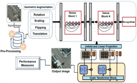
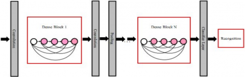
Figure 1 shows the proposed framework for vehicle type detection, combining geometric augmentations and transformers with densely connected convolutional layers. As a preprocessing step, the input remote sensing images are rotated, scaled and flipped through geometric augmentations. This process helps to work with diverse orientations in aerial images. The ability of the model to learn spatial distortion and work in different imaging conditions is possible through geometric augmentations.
Figure 1. Block diagram of proposed model Dense-TNT
Next step is to process the images through DenseNet blocks for feature extraction through dense connectivity which also facilitates the stable flow of gradient. This process can be used to recognize even overlapping vehicles that are smaller in size. Then the generated feature maps are given as input to Transformer-in-Transformer module the core component of the framework. The fine grained patch relationships of the feature maps are captured by inner transformer layers. Then the outer transformer layer captures the broader dependencies of patches across different scenes based on the given input images. The attention mechanism of the transformer architecture helps the model in learning detailed representation of the images. This process helps to differentiate same category of vehicles in different backgrounds.
Next step is to construct unified feature representation by fusing the patch embeddings of inner and outer transformers Finally the classification head uses this feature representation to identify the vehicle types. The accuracy of the process is improved through the use of geometric augmentation for feature extraction, and encoding of inner and outer transformers and classification. Through this approach the proposed hybris model provides better accuracy and scalability in detecting vehicle types in remote sensing images.
3.1 Problem analysis
The main objective is to combine CNN and ViT versions in order to create an end-to-end vehicle detection mechanism. Using satellite RS photos of different vehicle types taken in different locations and with different weather circumstances, the suggested model does image processing and produces better results for vehicle type detection.
3.2 Pre-processing
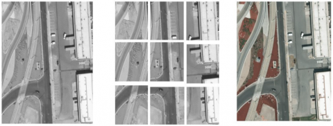
The image size in the experiment varies based on the reconstruction scale after the image has been rebuilt [9]. For example, an image that was 800 × 800 pixels before reconstruction is now 1600 × 1600 pixels. The object detection result is displayed in Figure 2, where the red square in the right photos represents the border. This change is applied during the object detection phase to maintain compatibility with the original method input size and avoid detection problems for small objects caused by image scaling.
Figure 2. Schematic diagram of image pre-processing
To minimize the loss of edge object data during images segmentation, the initial step involves segmenting the image using overlapping sliding windows. The input image has dimensions of 1600 × 1600 pixels, the segmentation step size is 600 pixels, and the overlapped region measures 200 pixels. This process results in nine final image slices, each measuring 800 × 800 pixels. The following formula can be utilized to compute the number of images slices produced after segmentation:
$b=(W D-w d) /\left(w d-w d_1\right)+1$ (1)
$a=(H T-h t) /\left(h t-h t_1\right)+1$ (2)
where, WD and HT are the width and height of the original image size, correspondingly. wd and ht are the width and height of the image slice, correspondingly; wd1 and ht1 are the width and height of the overlapping region, correspondingly, though b and a are the number of rows and columns in the images slice.
Second, the segmented images are concatenated during the object diagnosis phase, to prevent the repetitive identification of cars in overlapping areas. For instant results, the separated images are sent to the object detection process. These images are then excluded from accessing the diagnosis outcomes of the original images. The objects identified based on positional data within the image slices are mapped back to the absolute coordinates of the original images using Eqs. (1) and (2). The fusion technique uses these equations to determine the relative location of the picture slice's upper-left corner and the matching coordinates in the original images. The final detection results are obtained when the NMS (Non-Maximum Suppression) technique is applied to remove redundant diagnosis outcomes caused by overlapping regions, especially for the outcomes near the edges of the image fusion.
3.3 Geometric augmentations
In order to overcome the challenges in remote sensing data, geometric augmentations like scaling and rotation applied to training images. These augmentations include:
Rotations:
$I\left(x^{\prime}, y^{\prime}\right)=I(x \cos \theta-y \sin \theta, x \sin \theta+y \cos \theta)$ (3)
Scaling:
$I^{\prime}(x, y)=I\left(s_x x, s_y y\right)$ (4)
where, $s_x$ and $s_y$ are scaling factors.
Flipping: Horizontal or vertical inversions are used to diversify the training data.
Translation: Shifting image pixels by transformations $T_x$ and $T_y$.
These transformations enable the model to learn invariant features under diverse conditions.
3.4 Dense-TNT architecture
The Dense-TNT architecture combines two powerful computational frameworks: DenseNet and the TNT model. This hybrid approach is specifically designed to tackle the challenges of vehicle type detection in remote sensing images, where both local detail and global context are crucial for accurate detection and classification. Below is a detailed theoretical breakdown of its components:
3.4.1 DenseNet for local feature extraction
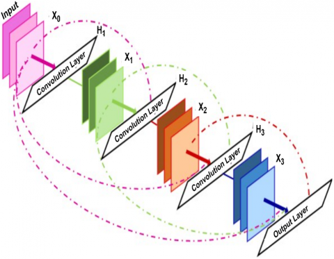
As mentioned in the previous sections, CNNs' use of convolution procedures and kernel structures usually results in better local fixed information extraction capabilities [16]. Therefore, when creating our efficient image recognition model, we kept the convolutional layer. In this work, DenseNet was used as the localisation information extractor to address the issue of losing fine-grained localisation features. For the purpose of obtaining localised spatial information, DenseNet was created especially. Different ResNet and other popular CNN models that use sequential connections between layers, DenseNet employs a feed-forward network to connect each convolutional layer to every other layer. This approach is referred to as dense connectivity [17].
This can be mathematically expressed as:
$Z_i^*=H_i\left(\left[Z_0, Z_1, \ldots \ldots, Z_{i-1}\right]\right)$ (5)
where, $H_i(i)$ represents a composite function consisting of convolution, batch standardization, and a ReLU activation function. The concatenation of feature maps from preceding levels ensures:
The vanishing gradient problem is addressed in the proposed approach and the feature maps of previous convolution layers are utilized by every layer. This approach preserves dependencies being lost during feature extraction. These features are essential to handle complexity of the data during conditions such as low light environment and cloudy weather.The detailed architecture of the deep learning model used in the proposed approach, DenseNet is specified in Figure 3. The architecture reveals that the feature maps of earlier stages are passed to every layer in the architecture. Moreover, the feature map size can be modified through the convolution layers present between two adjacent blocks of the DenseNet architecture.
Figure 3. DenseNet model structure diagram
3.4.2 Transformer-in-Transformer for global contextual understanding
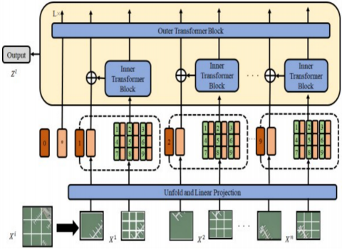
The ability of ViT to extract global long-sequence dependencies has enabled its successful application in various contexts, demonstrating its efficiency. However, ViT and CNNs still exhibit differences in their performance when it comes to local information aggregation. Combining ViT with CNNs provides a simpler approach to equipping transformer architectures with the ability to capture local data, even though several studies have proposed modifications to enhance ViT's local extraction capabilities. The design of TNT is illustrated in Figure 4.
Figure 4. Transformer-in-Transformer (TNT) architecture model
Similarly, TNT [18] was chosen as the substitute for our suggested hybrid model following a thorough review of the literature. The Transformer finds it difficult to identify relationships based only on the 2D patch layout, even if the usual ViT architecture splits input images into long sequence patches without taking local correlation data into account. As the name implies, the TNT design uses an exterior Transformer to spread information between patches and an inside Transformer to simulate the correlations between sub-patches. A hierarchical structure is embedded in TNT:
Patch and Sub-Patch Division: Each image is divided into patches, and to capture finer details, each patch is further subdivided into sub-patches.
Patches are treated as "visual sentences” $\left(X_i\right)$, and sub-patches as "visual words” $\left(Y_i\right)$, embedded hierarchically:
$X_i \rightarrow Y_i=\left[y_{i, 1}, y_{i, 2}, \ldots, y_{i, m}\right]$ (6)
Internal Transformer for Local Attention: The internal transformer operates within sub-patches to model local relationships.
$Y_i^{\prime}=Y_{i-1}+{MSA}\left(L N\left(Y_{i-1}\right)\right)$ (7)
$Y_i=Y_i^{\prime}+M L P\left(L N\left(Y_i^{\prime}\right)\right)$ (8)
Here, MLP stands for Multi-Layer Perceptron, LN for Layer Normalization, and MSA for Multi-Head Self-Attention.
External Transformer for Global Attention: The external transformer models global interactions between patches:
$Z_i^{\prime}=Z_{i-1}+{MSA}\left(L N\left(Z_{i-1}\right)\right)$ (9)
$Z_i=Z_i^{\prime}+M L P\left(L N\left(Z_i^{\prime}\right)\right)$ (10)
In order to retain global spatial relationships, the hierarchical mechanism enables TNT to preserve localized details.
3.4.3 Dense-TNT overview model
Finally, hybrid TNT and DenseNet model has been proposed as shown in Figure 4. The convolutional layer is used to extract local fixed features, the transformer-based layer is used to ensure robust baseline performance. TNT architecture is more effective at capturing global data and provides a better comprehension than standard ViT. The convolution and kernel process makes DenseNet excel in image recognition by providing deeper localized feature extraction ability than CNN variants. Through the process of extracting local features from the data processed by this hybrid structure, the proposed Dense-TNT model can further enhance recognition performance under challenging environmental conditions. The proposed Dense-TNT neural network, composed of DenseNet and TNT components, is illustrated in Figure 5. The recognition layer serves as the classifier, determining the likelihood of the input vehicle's variety. Additional learnable embeddings in the example are indicated by the symbol *.
Figure 5. The design of the proposed Dense-TNT neural network
|
Algorithm 1: Pseudocode for Dense-TNT proposed model |
|
Input: Remote sensing images dataset (D), augmentation parameters $\left(\theta, T_x, T_y, s_x, s_y\right)$ Output: Predicted vehicle type probabilities (O) Step 1: Data Pre-processing FOR each image I in dataset D: Apply Geometric Augmentations I_rotated = Rotate (I, θ) # θ: rotation angle I_scaled = Scale $\left(I, s_x, s_y\right)$ # $s_x, s_y$: scaling factors I_flipped = Flip (I) # Horizontal or vertical flip I_translated = Translate $\left(I, T_x, T_y\right)$ # $T_x, T_y$: translation offsets Normalize (I_augmented) # Normalize pixel values to [0, 1] Divide I_augmented into patches {$X_1, X_2, \ldots, X_n$} FOR each patch $X_i$: Divide $X_i$ into sub-patches {$y_{i, 1}, y_{i, 2}, \ldots, y_{i, m}$} Step 2: Dense-TNT Model DenseNet Module (Local Feature Extraction) FOR layer i in DenseNet layers: $Z_i^*=H_i\left(\left[Z_0, Z_1, \ldots \ldots, Z_{i-1}\right]\right)$ $H_i$ includes Convolution, BatchNorm, ReLU TNT Module (Global Feature Extraction) FOR patch $X_i$ in {$X_1, X_2, \ldots, X_n$}: # Internal Transformer: Local correlations within sub-patches $Y_i^{\prime}=Y_{i-1}+\operatorname{MSA}\left(L N\left(Y_{i-1}\right)\right)$ $Y_i=Y_i^{\prime}+M L P\left(L N\left(Y_i^{\prime}\right)\right)$ External Transformer: Global correlations among patches $Z_i^{\prime}=Z_{i-1}+M S A\left(L N\left(Z_{i-1}\right)\right)$ $Z_i=Z_i^{\prime}+M L P\left(L N\left(Z_i^{\prime}\right)\right)$ Step 3: Classification Layer Compute feature vector Z* = Output (TNT) FOR each vehicle class i in {1, 2, ..., C}: $v_i=W^T Z+b$ # Eq. (9) $o_i=\frac{e^{v_i}}{\sum_{j=1}^C e^{v_j}}$ # Softmax normalization Step 4: Training and Evaluation $ComputeLoss=-\sum\left(y_i * log \left(o_i\right)\right)$ # Cross-entropy Loss between predicted probabilities O and ground truth labels Update model parameters using AdamW optimizer with settings Learning rate (α) = 1e-4 Beta1 (β1) = 0.9 Beta2 (β2) = 0.999 Weight decay (λ) = 1e-2 Batch size = 16 or 32 Evaluate model with Accuracy, Precision, Recall, F1-score Output vehicle type probabilities O for each input image |
3.5 Advantages of proposed model
4.1 Experiment settings
The following experiments maintained all parameters, including training and baseline models. ViT and PoolFormer were used as the baseline models. ViT is commonly used to solve image processing issues. ViT with two and twelve layers, PoolFormer with s12 and s24 parameter sizes, and Dense-TNT with s12 and s24 parameter sizes were all employed. The starting and Dense-TNT model variable combinations are shown in Table 1. The dense blocks of the Dense-TNT s12 and Dense-TNT s24 models consisted of five convolutional layers with 5 × 5 kernels and a stride of 1.
Table 1. Parameter settings [3]
|
Model |
Attention Heads (H) |
Hidden Size (D) |
Number of Layers (L) |
MLP Size |
|
PoolFormer s24 |
- |
512 |
24 |
- |
|
PoolFormer s12 |
- |
384 |
12 |
|
|
Vision Transformer (ViT-L/12) |
16 |
1024 |
12 |
4096 |
|
Vision Transformer (ViT-L/2) |
16 |
1024 |
2 |
4096 |
|
Dense-TNT s24 |
8 |
512 |
24 |
- |
|
Dense-TNT s12 |
8 |
384 |
12 |
- |
A computer with an i5-8600K CPU, a 1TB HDD, a GeForce 1050Ti 4GB GPU, 16GB of RAM, and a 250GB SSD was used to simulate the suggested model utilizing Python 3.6.5. The limitation settings are as follows: batch size: 5; epoch count: 50; learning rate: 0.01; dropout: 0.5; activation function: ReLU. The models used in this study include Faster-RCNN [19], YOLOv3 [20], AGMFNet [21], and TMAFNet [22].
4.2 Dataset description
Two benchmark datasets are utilized for the research evaluation of the Dense-TNT method: VEDAI [23] and ISPRS [24] Potsdam. The VEDAI dataset consists of 3,687 aerial images, primarily designed for vehicle detection tasks, providing diverse scenarios and challenging small object detection. The ISPRS Potsdam dataset, with 2,244 high-resolution aerial images, focuses on urban scene classification and segmentation, providing detailed annotations for buildings, vegetation, cars, and other urban features.
Table 2. Details for VEDAI dataset
|
Class |
Number of Images |
|
Van |
100 |
|
Pickup |
950 |
|
Plane |
47 |
|
Tractor |
190 |
|
Camping Car |
390 |
|
Boat |
170 |
|
Car |
1340 |
|
Other |
200 |
|
Truck |
300 |
|
Overall images |
3687 |
For a rigorous evaluation, both datasets are systematically partitioned into training, validation, and test sets. Specifically, 70% of the images are allocated for training, 15% for validation, and the remaining 15% for testing, ensuring that each split preserves the diversity and complexity of the scenes. This allocation allows for effective model learning, hyperparameter tuning, and unbiased assessment of generalization performance.
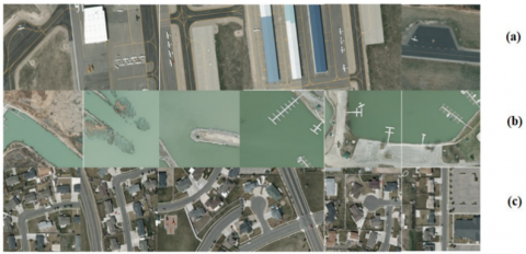
Tables 2 and 3 provide a comprehensive summary of these datasets, highlighting their characteristics such as image resolution, classes, and annotation details. Figure 6 illustrates representative samples from both datasets, showcasing the variety and complexity of the imagery used for Dense-TNT evaluation.
Table 3. Details on ISPRS Postdam dataset
|
Class |
Number of Images |
|
Van |
181 |
|
Pickup Car |
40 |
|
Truck |
33 |
|
Car |
1990 |
|
Overall images |
2244 |
Figure 6. Sample images for dataset: (a) Plane, (b) Boat, (c) Car
4.3 Performance evaluation metrics
Precision quantifies the percentage of true positive forecasts correctly identified positives out of all positive forecasts made by a model. It indicates the accuracy of favourable predictions.
$Precision=\frac{T P}{T P+F P}$ (11)
A model's recall quantifies its ability to accurately identify every relevant instance. It is sometimes referred to as the true positive rate or sensitivity.
$Re c all=\frac{T P}{T P+F N}$ (12)
The F-Score, also known as the F1-Score, is the harmonic mean of recall and precision. It evaluates the balance between these two metrics in a classification task, particularly when the data is unbalanced. It is most effective when the costs of false positives and false negatives differ.
$F- Score =2 \times \frac{{Precision} \times {Recall}}{{Precision}+{Reccall }}$ (13)
The Matthews Correlation Coefficient (MCC) is a statistical metric used to evaluate the quality of binary classifications, considering true negatives (TN), false positives (FP), false negatives (FN), and true positives (TP). It provides a balanced score even in cases with unequal class distributions.
$M C C=\frac{(T P \times T N)-(F P \times F N)}{\sqrt{(T P+F P)(T P+F N)(T N+F P)(T N+F N)}}$ (14)
FPS (Frames Per Second) is the number of individual frames or images displayed each second in a movie or animation. It is a metric for assessing how smooth the motion appears in a video.
$F P S=\frac{ { Number~of~Frames~Displayed }}{ { Time~in~ Sec o nds }}$ (15)
A model's accuracy is a performance metric that represents the percentage of correct forecasts compared to the overall number of forecasts.
$Accuracy=\frac{T P+T N}{T P+T N+F P+F N}$ (16)
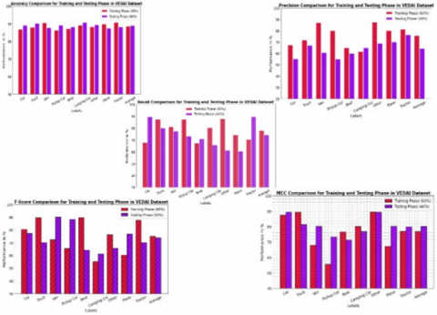
Table 4 and Figure 7 summarize the performance of the Dense-TNT technique for vehicle classification on the VEDAI dataset, evaluated across multiple metrics: Accuracy, Precision, Recall, F-Score, and MCC. The model's presentation was assessed during both the training phase (60% of the dataset) and the testing phase (40%). The Car class demonstrated robust Accuracy of 89.12% during testing, an improvement from 86.98% during training. The Precision values as been dropped in the testing phase (55.32%) compared to training (67.45%). It has been observed that the Truck class shows better accuracy of 90.23% in testing. For Van class, Accuracy dropped slightly from 90.66% during training to 87.76% in testing. The reduction in Precision and Recall, shows challenges in generalizing this class. Throughout testing, the Pickup Car class showed increased accuracy (89.22%) but decline in precision and recall. While the F-Score and MCC metrics showed minor discrepancies, indicating potential for improvement, the Boat and Camping Car classes indicated steady increases in accuracy during testing (88.33% and 90.99%, respectively). Throughout the combined phases, the other class maintained strong MCC values and steady accuracy (89.44%), demonstrating great reliability. Throughout the testing phase, both the Plane and Tractor classes demonstrated excellent performance; the Tractor class maintained high Recall and MCC values in spite of minor training-related reductions in Precision. Although there is a noticeable drop in Precision and Recall after testing, the average values for all classes show stable overall Accuracy (88.99%), indicating opportunities for improvement in balancing these metrics. Total, the Dense-TNT method established reliable presentation, efficiently classifying vehicles on the VEDAI dataset, with testing metrics affirming its generalization abilities. However, variations in Precision and Recall across specific classes indicate potential opportunities for optimization. Results indicate that differences in accuracy and MCC between training and testing are generally not statistically significant (p > 0.05), confirming robust generalization. However, precision for small-object classes (e.g., Car, Pickup Car) shows a modest but significant drop in the testing phase (p < 0.05), highlighting challenges in small vehicle detection. The Dense-TNT model shows strong overall accuracy on the VEDAI dataset (88.99%), but performance varies across classes; notably, the Van class experiences a drop in accuracy, precision, and recall during testing, highlighting areas where the model’s generalization could be further optimized.
Figure 7. Vehicle classifier outcome of Dense-TNT technique on VEDAI dataset
Table 4. Vehicle classifier outcome of Dense-TNT technique on VEDAI dataset [6, 22]
|
Labels |
Accuracy |
Precision |
Recall |
F-Score |
MCC |
|
Training Phase (60%) |
|||||
|
Car |
86.98 |
67.45 |
67.76 |
80.44 |
87.44 |
|
Truck |
88.11 |
71.98 |
87.33 |
89.54 |
89.23 |
|
Van |
90.66 |
87.33 |
81.11 |
72.21 |
67.88 |
|
Pickup Car |
86.45 |
80.22 |
87.33 |
65.34 |
55.44 |
|
Boat |
87.33 |
65.23 |
67.22 |
89.54 |
76.65 |
|
Camping Car |
89.23 |
61.76 |
80.33 |
55.23 |
80.11 |
|
Other |
88.44 |
87.76 |
87.83 |
76.22 |
89.55 |
|
Plane |
89.91 |
80.22 |
74.23 |
60.22 |
67.23 |
|
Tractor |
90.91 |
81.55 |
70.34 |
87.44 |
76.87 |
|
Training Phase (60%) |
|||||
|
Car |
89.12 |
55.32 |
89.43 |
77.33 |
89.23 |
|
Truck |
90.23 |
67.23 |
80.22 |
70.11 |
81.22 |
|
Van |
87.76 |
60.98 |
77.44 |
89.98 |
80.33 |
|
Pickup Car |
89.22 |
55.12 |
73.34 |
88.23 |
73.35 |
|
Boat |
88.33 |
59.98 |
70.98 |
64.34 |
71.22 |
|
Camping Car |
90.99 |
65.23 |
65.87 |
61.22 |
76.76 |
|
Other |
89.44 |
68.98 |
61.22 |
65.66 |
89.23 |
|
Plane |
87.54 |
70.23 |
60.55 |
76.87 |
80.33 |
|
Tractor |
88.33 |
76.65 |
89.76 |
70.22 |
79.91 |
Table 5. Comparative analysis of performance metrics on VEDAI dataset
|
Methods |
Accuracy |
Precision |
Recall |
F-Score |
MCC |
|
Dense-TNT (Proposed) |
88.99 |
64.41 |
74.31 |
73.77 |
80.17 |
|
Faster-RCNN |
76.34 |
54.99 |
65.89 |
61.18 |
74.23 |
|
YOLOv3 |
81.33 |
50.55 |
61.11 |
70.34 |
72.88 |
|
AGMFNet |
74.23 |
62.77 |
72.33 |
67.76 |
69.91 |
|
TMAFNet |
65.39 |
60.91 |
70.21 |
66.23 |
62.44 |
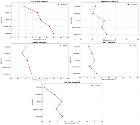
Table 5 and Figure 8 compare performance metrics for several techniques on the VEDAI dataset, emphasizing the superiority of the proposed Dense-TNT model. Dense-TNT achieved the highest accuracy (88.99%), precision (64.41%), recall (74.31%), F-score (73.77%), and Matthews Correlation Coefficient (MCC, 80.17%), demonstrating consistent performance across all parameters. In contrast, Faster-RCNN, YOLOv3, AGMFNet, and TMAFNet exhibited lower performance, with accuracy ranging from 65.39% to 81.33% and MCC values ranging from 62.44 to 74.23. These results highlight Dense-TNT's effectiveness in addressing challenges with the VEDAI dataset.
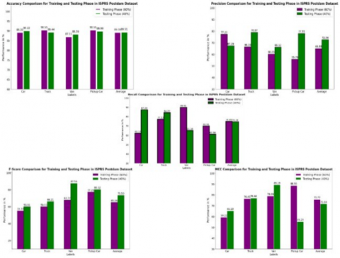
Table 6 and Figure 9 present the performance evaluation of the Dense-TNT technique for vehicle classification on the ISPRS Potsdam dataset. The table compares organization metrics, including Accuracy, Precision, Recall, F-Score, and MCC, during the training phase (60% of the data) and testing phase (40% of the data) for four vehicle categories: Car, Truck, Van, and Pickup Car. Across all categories, the Dense-TNT technique demonstrates strong performance, with average Accuracy reaching 89.38% in the training phase and slightly improving to 89.51% in the testing phase. Precision and Recall show balanced values, with averages of 64.88% and 74.83% during training and 72.54% and 74.44% during testing, respectively. The F-Score and MCC values indicate consistent classification reliability, achieving averages of 65.06 and 75.77 during training and 73.50 and 71.64 during testing. Among individual categories, the classification of "Truck" stands out with a high Recall (77.33%) during training, while "Pickup Car" demonstrates a strong F-Score (80.32%) during testing. These findings underscore the Dense-TNT technique's resilience and versatility in accurately recognizing various vehicle types under diverse environmental conditions.
Figure 8. Comparative analysis of performance metrics on VEDAI dataset
Table 6. Vehicle classifier outcome of Dense-TNT technique on ISPRS Postdam dataset [6]
|
Labels |
Accuracy |
Precision |
Recall |
F-Score |
MCC |
|
Training Phase (60%) |
|||||
|
Car |
89.33 |
77.23 |
62.17 |
55.33 |
59.22 |
|
Truck |
90.55 |
66.33 |
77.33 |
59.91 |
76.45 |
|
Van |
87.11 |
60.23 |
89.91 |
67.77 |
78.89 |
|
Pickup Car |
90.55 |
55.76 |
69.91 |
77.23 |
88.55 |
|
Car |
89.33 |
77.23 |
62.17 |
55.33 |
59.22 |
|
Training Phase (60%) |
|||||
|
Car |
67.29 |
87.39 |
59.91 |
65.19 |
67.29 |
|
Truck |
78.87 |
84.22 |
66.21 |
76.98 |
78.87 |
|
Van |
66.12 |
65.18 |
87.56 |
89.19 |
66.12 |
|
Pickup Car |
77.91 |
60.98 |
80.32 |
55.23 |
77.91 |
|
Car |
67.29 |
87.39 |
59.91 |
65.19 |
67.29 |
Table 7. Comparative analysis of performance metrics on ISPRS Postdam dataset
|
Methods |
Accuracy |
Precision |
Recall |
F-Score |
MCC |
|
Dense-TNT (Proposed) |
89.51 |
72.54 |
74.44 |
73.50 |
71.64 |
|
Faster-RCNN |
86.76 |
68.33 |
72.91 |
69.13 |
66.54 |
|
YOLOv3 |
80.33 |
70.22 |
71.44 |
72.87 |
70.22 |
|
AGMFNet |
78.33 |
60.31 |
67.87 |
67.89 |
68.17 |
|
TMAFNet |
68.21 |
62.87 |
70.34 |
61.18 |
65.98 |
Figure 9. Vehicle classifier outcome of Dense-TNT technique on ISPRS Postdam dataset
Figure 10. Comparative analysis of performance metrics on ISPRS Postdam dataset
Table 7 and Figure 10 present a comparative analysis of performance metrics for various methods evaluated on the ISPRS Potsdam dataset. The proposed Dense-TNT method achieves the highest accuracy (89.51%) and consistently outperforms others across precision (72.54%), recall (74.44%), F-score (73.50%), and MCC (71.64%), highlighting its robustness in balancing predictive performance. Faster-RCNN, a widely used object detection framework, demonstrates moderate performance with an accuracy of 86.76% and a precision-recall trade-off slightly inferior to Dense-TNT. YOLOv3, known for real-time object detection, shows slightly lower accuracy (80.33%) but a relatively competitive F-score (72.87%) and MCC (70.22%), suggesting effective detection with limitations in precision. AGMFNet and TMAFNet, while yielding acceptable recall rates, underperform in accuracy and F-score compared to Dense-TNT, with TMAFNet showing the weakest overall metrics. These results underscore Dense-TNT's superiority in leveraging advanced architectural strategies for high-resolution aerial imagery tasks.
Table 8. FPS (Frames per Second) analysis for Dense-TNT technique with existing systems
|
Methods |
FPS |
|
Proposed |
1.654 |
|
Faster-RCNN |
9.887 |
|
YOLOv3 |
8.113 |
|
AGMFNet |
7.335 |
|
TMAFNet |
5.876 |
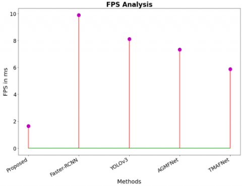
Figure 11. FPS (Frames per Second) analysis for Dense-TNT technique with existing systems
Table 8 and Figure 11 present the FPS (Frames Per Second) analysis comparing the Dense-TNT technique with existing systems. The suggested technique achieves an FPS of 1.654, which is significantly lower than that of other systems, including Faster-RCNN (9.887), YOLOv3 (8.113), AGMFNet (7.335), and TMAFNet (5.876). Although Dense-TNT achieves high accuracy, its lower FPS may limit real-time applicability, and further evaluation is needed to determine suitability for practical deployment. The proposed technique operates at a reduced frame rate, this trade-off may indicate a focus on accuracy or computational complexity, highlighting its unique advantages in specific applications compared to faster but potentially less precise methods.
4.4 Ablation study
The ablation study on the Geometric Augmentations-based Dense-TNT model highlights the impact of various components on its performance in vehicle type detection within RS images. The baseline Dense-TNT model achieves moderate accuracy; nevertheless, integrating geometric augmentations such as rotations, scaling, flipping, and their combinations significantly improves its robustness against variations in vehicle orientation, size, and positioning. The arrangement of all augmentations provides the best overall display, but flipping achieves the most accuracy among individual augmentations. This highlights the crucial part geometric augmentations play in improving the model's generalisation to a variety of real-world situations, which raises the accuracy and dependability of its detection.
Table 9. Ablation study for proposed model
|
Technique |
Accuracy |
|
Baseline (Dense-TNT) |
78.54 |
|
Dense-TNT + Geometric Augmentations (Rotations) |
84.34 |
|
Dense-TNT + Geometric Augmentations (Scaling) |
70.16 |
|
Dense-TNT + Geometric Augmentations (Flipping) |
86.44 |
|
Dense-TNT + All Geometric Augmentations |
89.25 |
Table 9 and Figure 12 show the results of an ablation research that investigated the effect of geometric augmentations on the accuracy of the Dense-TNT model for vehicle type diagnosis. The baseline model achieves an accuracy of 78.54%, which can be greatly improved by applying individual geometric augmentations. Between the augmentations, flipping has the best accuracy (86.44%), followed by rotation (84.34%). Scaling results in a rather low development, with an accuracy of 70.16%. When all augmentations are merged, the model achieves its highest accuracy of 89.25%, demonstrating the effectiveness of using multiple geometric changes to improve model robustness and presentation.
Figure 12. Ablation study for proposed model
4.5 Limitations and challenges
While Geometric Augmentations-based Dense-TNT produces promising results for vehicle type detection in RS pictures, it has significant limits and problems. The computational complexity of the Dense-TNT architecture may result in faster training times and higher resource requirements, making it unsuitable for real-time or resource-constrained queries. Furthermore, relying on geometric augmentations may not adequately address instances with severe fluctuations in image quality, lighting conditions, or occlusions. Data scarcity for specific vehicle kinds in remote sensing dataset containers further limits the model's capacity to generalize across various contexts. Balancing model robustness with computing efficacy remains a significant problem for wider use in real-world contexts.
A method integrating geometric augmentations with the Dense-TNT architecture was proposed in order to enhance vehicle type detection in remote sensing images. Geometric augmentations, were utilized to overcome the challenges arising from variations in scale and orientation. The proposed model, combining DenseNet for local feature extraction with TNT mechanism for global spatial dependency modeling, improves accuracy of detection compared to existing approaches. The model exhibits reduced precision for small or similar vehicle classes, and its lower FPS may restrict real-time applicability.
Future work includes incorporating advanced data augmentation techniques, such as generative adversarial networks (GANs), to address lack of data and improve robustness. The integration of multi-modal data, including LiDAR and thermal imagery, could enhance detection under challenging environmental conditions. Also, developing lightweight Dense-TNT variants may enable real-time deployment on edge devices, to apply in diverse real-time environments.
|
X |
Patch |
|
Y |
Sub patch |
|
WD |
width |
|
HT |
height |
|
X |
Mean |
|
MSA |
Multihead Self Attention |
|
MLP |
Multilayer Perceptron |
|
oj |
Softmax normalization |
|
TNT |
Transformer in Transformer |
|
ReLU |
Residual connection |
|
TP, TN |
True Positive, True Negative |
|
FP, FN |
False Positive, False Negative |
|
Greek symbols |
|
|
λ |
Weight decay |
|
α, β1, β2 |
Learning rate |
[1] Chen, Y., Qin, R., Zhang, G., Albanwan, H. (2021). Spatial temporal analysis of traffic patterns during the COVID-19 epidemic by vehicle detection using planet remote-sensing satellite images. Remote Sensing, 13(2): 208. https://doi.org/10.3390/rs13020208
[2] Zhou, W., Shen, J., Liu, N., Xia, S., Sun, H. (2022). An anchor-free vehicle detection algorithm in aerial image based on context information and transformer. IEEE Geoscience and Remote Sensing Letters, 19: 1-5. https://doi.org/10.1109/LGRS.2022.3202186
[3] Punithavathi, I.H., Dhanasekaran, S., Duraipandy, P., Lydia, E.L., Sivaram, M., Shankar, K. (2022). Optimal dense convolutional network model for image classification in unmanned aerial vehicles based ad hoc networks. International Journal of Ad Hoc and Ubiquitous Computing, 39(1-2): 46-57. https://doi.org/10.1504/IJAHUC.2022.120944
[4] Karnick, S., Ghalib, M.R., Shankar, A., Khapre, S., Tayubi, I.A. (2022). A novel method for vehicle detection in high-resolution aerial remote sensing images using YOLT approach. Multimedia Tools and Applications, 81(17): 23551-23566. https://doi.org/10.1007/s11042-022-12613-9
[5] Hoanh, N., Pham, T.V. (2024). A multi-task framework for car detection from high-resolution uav imagery focusing on road regions. IEEE Transactions on Intelligent Transportation Systems, 25(11): 17160-17173.
[6] Shen, J., Liu, N., Sun, H. (2021). Vehicle detection in aerial images based on lightweight deep convolutional network. IET Image Processing, 15(2): 479-491. https://doi.org/10.1049/ipr2.12038
[7] Kumar, S., Jain, A., Rani, S., Alshazly, H., Idris, S.A., Bourouis, S. (2022). Deep neural network based vehicle detection and classification of aerial images. Intelligent Automation & Soft Computing, 34(1): 119-131. https://doi.org/10.32604/iasc.2022.024812
[8] Upadhye, S., Neelakandan, S., Thangaraj, K., Babu, D.V., Arulkumar, N., Qureshi, K. (2023). Modeling of real time traffic flow monitoring system using deep learning and unmanned aerial vehicles. Journal of Mobile Multimedia, 19(2): 477-496. https://doi.org/10.13052/jmm1550-4646.1926
[9] Zhu, H., Lv, Y., Meng, J., Liu, Y., Hu, L., Yao, J., Lu, X. (2023). Vehicle detection in multisource remote sensing images based on edge-preserving super-resolution reconstruction. Remote Sensing, 15(17): 4281. https://doi.org/10.3390/rs15174281
[10] Wu, X., Li, W., Hong, D., Tian, J., Tao, R., Du, Q. (2020). Vehicle detection of multi-source remote sensing data using active fine-tuning network. ISPRS Journal of Photogrammetry and Remote Sensing, 167: 39-53. https://doi.org/10.1016/j.isprsjprs.2020.06.016
[11] Ageed, Z.S., Yasin, H.M., Rashid, Z.N., Zeebaree, S.R. (2023). Leveraging high resolution remote sensing images for vehicle classification using sea lion optimization with deep learning model. Journal of Smart Internet of Things, 2022(1): 97-113. https://doi.org/10.2478/jsiot-2022-0007
[12] Qiu, Z., Bai, H., Chen, T. (2023). Special vehicle detection from UAV perspective via YOLO-GNS based deep learning network. Drones, 7(2): 117. https://doi.org/10.3390/drones7020117
[13] Javadi, S., Dahl, M., Pettersson, M.I. (2021). Vehicle detection in aerial images based on 3D depth maps and deep neural networks. IEEE Access, 9: 8381-8391. https://doi.org/10.1109/ACCESS.2021.3049741
[14] Momin, M.A., Junos, M.H., Mohd Khairuddin, A.S., Abu Talip, M.S. (2023). Lightweight CNN model: automated vehicle detection in aerial images. Signal, Image and Video Processing, 17(4): 1209-1217. https://doi.org/10.1007/s11760-022-02328-7
[15] Li, Z., Liang, H., Wang, H., Zheng, X., Wang, J., Zhou, P. (2023). A multi-modal vehicle trajectory prediction framework via conditional diffusion model: A coarse-to-fine approach. Knowledge-Based Systems, 280: 110990. https://doi.org/10.1016/j.knosys.2023.110990
[16] She, X., Zhang, D. (2018). Text classification based on hybrid CNN-LSTM hybrid model. In 2018 11th International symposium on computational intelligence and design (ISCID), Hangzhou, China, pp. 185-189. https://doi.org/10.1109/ISCID.2018.10144
[17] Huang, G., Liu, Z., Van Der Maaten, L., Weinberger, K.Q. (2017). Densely connected convolutional networks. In Proceedings of the IEEE Conference on Computer Vision and Pattern Recognition, pp. 4700-4708.
[18] Han, K., Xiao, A., Wu, E., Guo, J., Xu, C., Wang, Y. (2021). Transformer in transformer. Advances in Neural Information Processing Systems, 34: 15908-15919. https://proceedings.neurips.cc/paper_files/paper/2021/file/854d9fca60b4bd07f9bb215d59ef5561-Paper.pdf.
[19] Zhang, H., Shao, F., Chu, W., Dai, J., Li, X., Zhang, X., Gong, C. (2024). Faster R-CNN based on frame difference and spatiotemporal context for vehicle detection. Signal, Image and Video Processing, 18(10): 7013-7027. https://doi.org/10.1007/s11760-024-03370-3
[20] Wang, K., Liu, M., Ye, Z. (2021). An advanced YOLOv3 method for small-scale road object detection. Applied Soft Computing, 112: 107846. https://doi.org/10.1016/j.asoc.2021.107846
[21] Gao, T., Li, Z., Wen, Y., Chen, T., Niu, Q., Liu, Z. (2023). Attention-free global multiscale fusion network for remote sensing object detection. IEEE Transactions on Geoscience and Remote Sensing, 62: 1-14. https://doi.org/10.1109/TGRS.2023.3346041
[22] Gao, T., Liu, Z., Zhang, J., Wu, G., Chen, T. (2023). A task-balanced multiscale adaptive fusion network for object detection in remote sensing images. IEEE Transactions on Geoscience and Remote Sensing, 61: 1-15. https://doi.org/10.1109/TGRS.2023.3289878
[23] Pepsissalom. (2023). VEDA: Vehicle Detection in Aerial Imagery Dataset [Data set]. Kaggle. https://www.kaggle.com/datasets/pepsissalom/vedaidataset.
[24] Kaggle. Datasets. https://www.kaggle.com/datasets, accessed on Jan. 5, 2026.