Aymen A. Hameed![]() | Noor Aldeen A. Khalid*
| Noor Aldeen A. Khalid*![]() | Ali Ibrahim Khaleel
| Ali Ibrahim Khaleel![]()
© 2025 The authors. This article is published by IIETA and is licensed under the CC BY 4.0 license (http://creativecommons.org/licenses/by/4.0/).
OPEN ACCESS
Recognition of traffic signs is essential in driving assistance systems, enabling drivers to better interpret their environment and prevent accidents. Important driving instructions and regulations, such as speed limits, pedestrian crossings, or upcoming turns, can be automatically detected by intelligent systems as part of the Advanced Driver-Assistance Systems (ADAS) dataset. Various automotive industry suppliers are actively developing this technology to minimize road sign misinterpretations and avoid accidents. This study applies image processing techniques for recognizing Chinese traffic signs, utilizing a dataset from a publicly available Chinese traffic sign recognition database. The paper evaluates the effectiveness of combining Histogram of Oriented Gradients (HOG) feature extraction with several classifiers, specifically Support Vector Machine (SVM), Decision Tree, and K-Nearest Neighbors (K-NN). This study addresses the challenge of real-time traffic sign recognition under variable conditions by proposing an ensemble method optimized for embedded systems. Results indicate that the HOG combined with the SVM classifier achieves the highest accuracy at 99.8%. Additionally, a voting classifier approach was explored, combining the outputs from K-NN, SVM, and Decision Tree classifiers to improve recognition accuracy. This ensemble approach significantly enhanced accuracy, achieving an accuracy of 99.996%, slightly higher than the SVM classifier alone at 99.994%. However, the voting classifier required more computational resources and had higher execution times. Eventually, the proposed traffic sign recognition method was tested on a Raspberry Pi embedded platform to assess practical applicability. Findings confirmed that while SVM slightly outperformed the other individual classifiers, the voting classifier provided higher overall accuracy, highlighting the advantages of ensemble methods in traffic sign recognition.
traffic sign recognition, HOG, SVM, ensemble learning, embedded systems, ADAS, Chinese traffic signs
The Intelligent Transportation System (ITS) is described as a system that uses communication and sensor techniques, advanced electronic equipment, to detect environmental situations and cars for drivers, which reduces the stress of driving and makes driving easier and safer. There are different devices, such as a computer vision system, ultrasonic waves, microwaves, radar, and infrared rays [1, 2].
Automatic traffic sign recognition (TSR) is an Advanced Driver Assistance Systems (ADAS). Traffic sign provides important graphical information such as; speed limitation, driving on proper lanes, lanes for pedestrians, roadway access, current traffic condition, avoiding obstacles, the direction of destination, etc. which help drivers while driving. Failure to notice traffic signs may indirectly or directly lead to traffic accidents [3]. A TSR system offers important information about the surroundings and traffic by recognizing and extracting feature the traffic signs which gives warning to drivers in any situation while the vehicle is running on the street [1]. There are several aspects that need to be taken into consideration while developing the TS, such as Variable lighting conditions, blurring and fading effects, impacted visibility, various signpost appearances, motion artefacts, disordered viewpoint and background, and a Sign that is partially obscured and impaired [4].
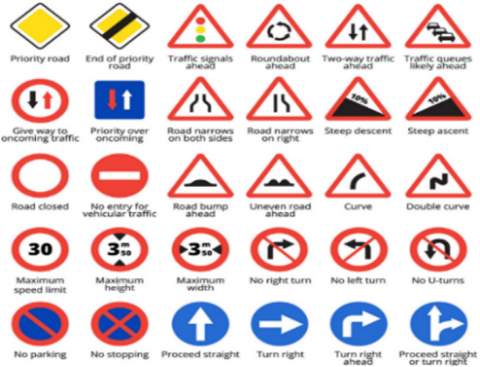
Traffic sign recognition is the technology that interprets the signs to the driver and also refers to as an assistance system. As shown in Figure 1, traffic signs are crucial for conveying essential information to drivers. Recognition is reliant on the combination of classification and detection [5]. Among the various methods available the one that is more important is chosen. Thus, detecting region of interest is achieved by using classification and Histogram of oriented gradient thereby using a support vector machine (SVM) [6].
Figure 1. Road traffic sign
Several paper and technical work have been done both in the academic and industrial areas on rendering, image processing, and perception. Topics like human perception of images and display optimization, image detection, recognition and classification are extremely important for both paper and development of popular products like TV sets, tablets, gaming devices, smartphones, digital cinema head-mounted displays, and traffic sign recognition and detection [7].
Image processing is a sort of signal processing in which an image, such as a photograph or video frame, serves as input, and a corresponding set of parameters relating to the image is produced as output, again in the form of a video frame or photograph. Numerous factors render image processing essential, including undesirable camera motion, an unsteady camera, or the need to compress a huge image for usage in certain applications [2].
The state of arts is an example of aforementioned method such as in the study [8] extraction of HOG and single classifier trained by ELM which has been used to acquire very highly efficient in computation and high recognition accuracy and by proposing an efficient technique for TSR that leverages one extreme learning machine (ELM) for multiclass identification after extracting variant HOG features from traffic signs. According to Liu et al. [9], the field sample collection used to trained the database in which the NN already trained the SGD optimizer utilized during training for learning efficiency by using a recognition framework named scale-aware TSR obtained high accuracy but the complexity high. The SVM methods incorporate the appropriate information, thereby demonstrating excellent performance regarding HSI classification which cooperates with a discrete space model (DSM). Another paper article Proposed a system that improved microarray images feature selection for cancer classification using K-NN based CPSO got accuracy between 83% to 100% in all dataset [10].
According to Eitel et al. [11], traffic sign recognition thus obtained varies from one group to another. More efforts are needed because of the non-availability of the standard datasets to determine the best among the methods. The system response cannot be predicted accurately based on certain circumstances like meteorological circumstances, misalignment of the sign, varying illumination levels, and occlusion [3]. Each paper uses its dataset having a minimum number of images thereby making the result less reliable due to the fact the specification as regarding the influence of images factors used in the experiment is not clear. Recently, few papers reveal their database, which includes images in large numbers that are compiled together to a database and made available for paper community.
In this paper use image processing methodologies to identify Chinese traffic signs, leveraging a dataset from a publicly accessible Chinese traffic sign recognition database. The study assesses the efficacy of integrating Histogram of Oriented Gradients (HOG) feature extraction utilizing diverse classifiers, comprising Support Vector Machine (SVM), Decision Tree, and K-Nearest Neighbors (K-NN) [12].
This paper structured as follow: Section 1 discusses how important it is for Advanced Driver-Assistance Systems (ADAS) to be able to recognize traffic signs. It also addresses the main contributions of the study and pertinent literature on traffic sign recognition methods and common classification Algorithms Section 2 hihglight the dataset that used for this study, going into detail on the features of the Chinese traffic sign database. It also explains the methods used, including how the data was prepared, the classification models (SVM, K-NN, and Decision Tree), and the ensemble voting system. Section 3 address the outcomes of the experimental results and the discussion, which includes evaluation metrics, comparisons of the accuracy of different classifiers, and the effectiveness of the ensemble approach.
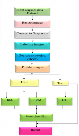
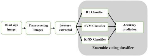
The proposed methodology in this paper has been applied to address the objectives of this study which is employed on The Chinese Traffic Sign Database, which available online (Traffic Sign Recognition Database). The proposed method uses the histogram of oriented gradients (HOG) as feature extraction and three classification algorithms then at the end multiply the result of these three algorithms by its weight and take the mean by using the voting algorithm, in order to achieve high accuracy. Before this step, the performance evaluation for the three algorithms should already exist. The development of the implementation was performed based on the OpenCV predefined and NumPy libraries that provide several images processing tasks. The evaluation of the algorithms based on image accuracy. In the hardware, the code done by Anaconda3 Python then attach the dataset and the code to the Raspberry Pi in order to assess the embedded system vs Spyder software (python) using execution time, the paper Schematic diagram is shown in Figure 2.
Figure 2. Schematic diagram of system operation
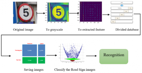
The proposed work includes three stages; image processing, classification, recognition as illustrated in Figure 3 the stage of image processing involved to convert the RGB image to gray scale image in order to avoid low vision and reduce the accuracy of image classification before the images need to be resized, in this process all the images be the same size for easy extracting feature and classification. The histogram of oriented gradient (HOG) is used to recognize the road sign by extracting features. Further one of the most important aspects training the images, that used thousands of images, this method used machine learning is to evaluate an algorithm by splitting a data set into two, one of those sets (the training set), on which learned some properties; which is the other set (the testing set), finally used three algorithms to classify trained images, by comparing the support vector machine (SVM) with other algorithms which are K-nearest neighbor and Decision Tree. Eventually, voting algorithm used to get high accuracy, the result of this algorithm and SVM compared with each other.
Figure 3. The process image recognition
2.1 Image dataset
The Traffic Sign Recognition Database (TSRD) consists of traffic sign images which are 6164 in number and comprises of 58 categories of traffic sign. The database where images are stored divided into two sub-databases as training database and testing database. The testing database includes 1994 images while the training database contains 4170 images. All images on the database annotated, i.e. the four coordinates of the sign and the category [13, 14]. To clarify the dataset and ensuring a fair assessment of model performance, the dataset is split into roughly 68% for training and 32% for testing.
A photo and image resizer is a superb tool that helps maintain websites, send images via email or resize large images for printing purposes. Aside from aiding in determining the size (in pixels) of an image, it also reduces the file size. In this paper, the image is resized to facilitate the process of feature extraction. All pictures used resized to the same x-dimension and y-dimension of (150*150) respectively.
2.2 Convert a color image to grayscale
An RGB image is also known as a color image. The pixels of a color image are determined by three values with each of the RGB (Red, Blue, and Green) components having one of the pixel scalar value. An M-by-N-by-3 array belonging to uint16, uint8, single, or double class whose pixel values defines the value of the intensity. For double or single arrays, the values range from 0 to 1 while uint8 values are within the range of 0 to 255 and class uint16 values range from 0 to 65535. It is also known as an intensity, grayscale, or gray level image. For the int16 class, values range from [-32768, 32767] [15, 16].
An image gray level denotes the quantization interval number in grayscale image processing. Presently, the most frequently used storage technique is 8-bit storage. An 8-bit grayscale image comprises of a number of gray levels (256) where Each pixel intensity varies from 0 to 255, with 0 representing black and 255 representing white. Another storage method that commonly used is 1-bit storage. This method consists of two gray levels, with which 0 is black, and 1 is white, and is mostly used in bio-medical images and referred to as binary image. Due to the fact that it is easy to work with binary images, images of other formats are mostly converted to binary format when used for edge detection or recognition, enhancement and so on [3]. In this study, RGB images were converted to grayscale, especially in traffic sign images because of weather fluctuation which might make the extraction of image features difficult. Furthermore, memory size reduced. There are several methods to convert an image to grayscale, but this work used a simple method which is a common method as shown in the equation below where the average value of the three colors (RGB) taken. Therefore, for a color image, the value of r is added to that of g and b then divided by 3 in order to achieve the desired image in grayscale format.
$Grayscale=\left( R+G+\frac{B}{3} \right)$ (1)
2.3 Histogram of Oriented Gradients (HOG)
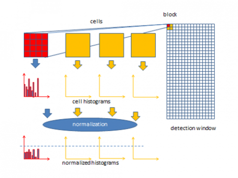
This is a feature descriptor that is used to find target objects in image processing and computer vision. The HOG descriptor counts the incidences of gradient orientation in the area localized in an image such as the Region of Interest (ROI) [17]. The implementation of HOG executed in some steps. Firstly, the image divided into small regions that are connected called cells. For every cell, HOG edge orientations or directions for pixels in the cell computed. After that, an individual cell discretized into angular bins in accordance with the orientation of the gradient. The pixel for individual cell delivers a weighted gradient to its matching angular bin. Moreover, sets of adjacent cells treated as blocks which are spatial regions. The grouping of cells into blocks is fundamental for the grouping and normalization of histograms. Lastly, histogram groups are normalized and denote the block histogram as shown in Figure 4.
Figure 4. The process of HOG
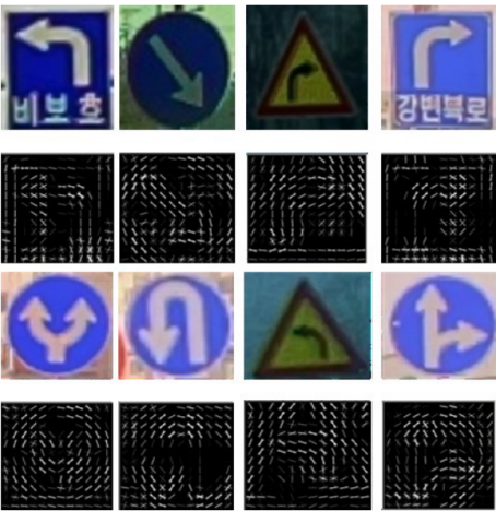
Practically, vertical and horizontal gradients are first calculated. The image split to cells of dimension 8×8, each of which HOG is derived. One of the major reasons feature descriptors are used to describe an image patch is because it provides a compact representation. The patch gradient comprises of two values (direction and magnitude) per pixel summing up to 8x8x2 = 128 numbers, to construct histogram of gradients in these 8×8 cells. This technique requires filtering the data intensity or color of the image with the following filter kernels as shown in Figure 5 and the HOG parameter listed in Table 1. To calculate the magnitude and direction of the gradient using the following formula
$\text{g}=\sqrt{\text{g}_{\text{x}}^{2}+\text{g}_{\text{y}}^{2}}$ (2)
$\text{ }\!\!\theta\!\!\text{ }=\text{arctan}\frac{{{\text{g}}_{\text{y}}}}{{{\text{g}}_{\text{x}}}}$ (3)
Figure 5. Training images for traffic sign recognition
Table 1. Configuration of HOG parameters in feature extraction
|
Parameters |
Value or Type |
|
Orientations |
8 |
|
Pixels per cell |
4*4 |
|
Cells per block |
2*2 |
|
Block norm |
L2 |
|
Visualize |
True |
2.4 Classification
Image classification algorithms used since the early 1970s when the information on land observation became accessible. Nearly all these algorithms range from the methods of visual interpretation to advanced machine learning algorithms. In this section, comparison between three algorithms done, and lastly, a voting algorithm is used to combine those three algorithms in order to enhance accuracy as shown in Figure 6.
Figure 6. Initialization of three exemplary classifiers for soft voting
2.4.1 Support Vector Machine (SVM)
Support Vector Machine (SVM) constructs a hyperplane or a collection of hyperplanes in a large or infinite-dimensional space applicable for various applications, including regression and classification. Intuitively, the hyper-plane which possesses the greatest distance to the closest training data nodes of any object class achieves a good separation which is referred to as functional margin. In general, the more the functional margin, the lesser the classifier’s generalization [18]. The SVM classifier defines as:
$min\frac{1}{2}{{w}^{T}}w+C\underset{i=1}{\overset{n}{\mathop \sum }}\,{{\zeta }_{i}}$ (4)
${{y}_{i}}\left( {{w}^{T}}\phi \left( {{x}_{i}} \right)+b \right)\ge 1-{{\zeta }_{i}},$ (5)
where, ${{\text{ }\!\!\zeta\!\!\text{ }}_{\text{i}}}\ge 0,\text{i}=1,\ldots .,\text{n}$, C > 0 is the upper bound, and (X, Y) stands for a group of feature vectors and a set of class labels in the training dataset respectively. W denotes the weight vector for learned decision hyperplane while b referred to as the model bias. ${{\zeta }_{i}}$ are the slack variables that demonstrate the distance of a particular instance from its proper side of the decision boundary in a geometric viewpoint, and it is a non-zero value for cases violating the constraint $\text{yi }\!\!~\!\!\text{ }\left( \text{w}.\text{xi }\!\!~\!\!\text{ }+\text{ }\!\!~\!\!\text{ b} \right)\text{ }\!\!~\!\!\text{ }\ge \text{ }\!\!~\!\!\text{ }1$. The C parameter is a trade-off amid minimization of error and maximization of margin, with a larger value of C putting more concentration on error minimization.
In this system, an SVM trained with Radial Basis Function (RBF) kernel, where two parameters C and gamma must be put into consideration. The parameter C, which is prevalent to all kernels in SVM, trades-off the misclassification of training samples against decision surface simplicity. A high C aims to correctly classify all training examples, while a low C smoothens the decision surface. Gamma defines the degree of influence of a sole training example. The bigger gamma is the nearer other samples must be for them to be affected. Where an appropriate choice of parameter gamma and C is significant to the performance of the SVM. To compute the RBF kernel between two vectors. The kernel defines as equation below.
$k\left( x,y \right)={{e}^{-\gamma {{\left| \left| y-x \right| \right|}^{2}}}}$ (6)
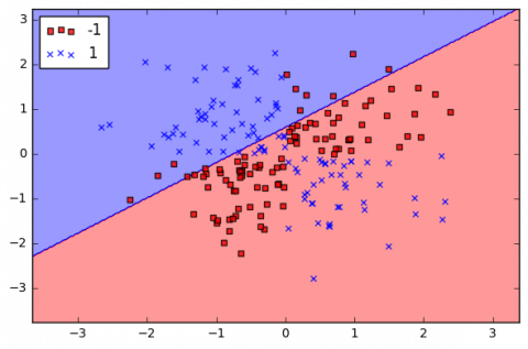
where, the x and y are the input vector and $\text{ }\!\!\gamma\!\!\text{ }$ is a slope, most of the time, the data will be composed of n vectors $\text{xi},$ for each xi will be related with a value$\text{ }\!\!~\!\!\text{ yi}$ showing whether the element belongs to the class (+1) or not (-1) as in Figure 7. Yi can only have two possible values -1 or +1. Moreover, most of the time, for instance when the text needs to be classified, the vector xi ends up having a lot of dimensions.$\text{ }\!\!~\!\!\text{ }xi$ is a p-dimensional vector provided it has p-dimensions as in Table 2. So, a dataset D is the set of n couples of elements $xi,yi$. Thus, the formal definition of an initial dataset in set theory is as follows:
$D=\left\{ \left( xi,yi \right)xi\in {{\mathbb{R}}^{p}},yi\in \left\{ -1,1 \right\} \right\}~{{i}^{2}}=1$ (7)
Figure 7. Data separated by an RBF kernel
Table 2. SVM parameter
|
SVM Parameter |
Values |
|
C |
1.0 |
|
Kernal |
Rbf |
|
Degree |
3 |
|
Gama |
Scale |
|
Shrinking |
True |
|
Probability |
True |
|
Tol |
0.001 |
|
Cashe_Size |
200 |
|
Verbose |
False |
|
Max_Iteration |
-1 |
|
Decision_Function_Shape |
Ovr |
2.4.2 Decision Trees (DTs)
Decision Trees is a method of supervised learning with no parameters which used for regression and classification [19, 20]. The aim of the Decision Tree is to create a model that guesses target variable values by studying simple decision guidelines that were deduced from the data features which can manage both categorical and numerical data and also requires little data preparation. Furthermore, it is adept in identifying multiple classes on a given dataset. Given the data at node m is denoted by $\text{Q}$, for any candidate split $\text{ }\!\!\theta\!\!\text{ }=\left( \text{j},\text{tm} \right)$ containing threshold $\text{tm}$ and a feature$\text{ }\!\!~\!\!\text{ j}$, segregate the data into $\text{Qleft}\left( \text{ }\!\!\theta\!\!\text{ } \right)$ and $\text{Qright}\left( \text{ }\!\!\theta\!\!\text{ } \right)$ subsets.
$Qleft\left( \theta \right)=\left( x,y \right)|{{x}_{j}}\le {{t}_{m}}$ (8)
$Qright\left( \theta \right)=Q\backslash Qleft\left( \theta \right)~$ (9)
2.4.3 K-Nearest Neighbour (KNN)
K-Nearest Neighbour is a well-known and often utilized algorithm in machine learning. Classification is performed based on the proximity of a chosen feature to the nearest one. The K value enables us to ascertain the volume of data to be evaluated based on the extent of data the categorization will generate. Eq. (11) delineates the distances between objects. Where the value of the n-neighbour is 10. Furthermore, the goal of KNN is to learn an optimal linear transformation matrix of size (components, features), This, as shown in the Eq. (10), maximizes the total across all samples i of an opportunity pi that i is properly identified.
$\begin{matrix} argmax \\ L \\\end{matrix}\underset{i=0}{\overset{N-1}{\mathop \sum }}\,pi$ (10)
$d\left( i,j \right)=\sqrt{\underset{k=1}{\overset{p}{\mathop \sum }}\,{{({{X}_{ik}}-{{X}_{jk}})}^{2}}}$ (11)
2.5 Voting classifier
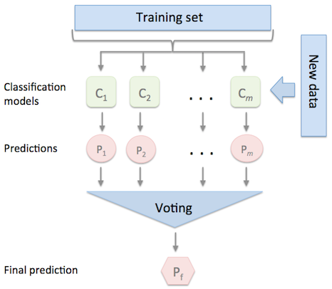
Conceptually combine diverse machine learning-based classifiers and use the mean predicted probabilities soft vote or majority vote to foretell the class labels. Hence, this classifier is suitable for a set of evenly well-performing models to stabilize their weaknesses. The class label returned as $\text{argmax}$ of the total predicted probabilities in soft voting. Figure 8 and Figure 9 indicate the voting steps.
Figure 8. Main steps of voting classifier
Figure 9. The voting classifier process
Certain weights could be allocated to every classifier via the weight’s parameter. As the weights allocated, the probabilities of the envisioned class for every classifier are collected, then multiplied by the weight of the classifier and lastly, the average is determined. Weights were assigned proportionally to each classifier’s standalone accuracy on the validation set. The resulting class label is obtained from the class label having the largest average probability. Three classifiers taken with three-class classification problems where several values of weights assigned to all classifiers. The class with the highest average probability chosen as the predicted class label.
2.5.1 Hard voting
In hard voting, they assign the final class label as the class label most commonly expected by classification models. Hard voting is the easiest vote-majority scenario. Which predicts the class tag $\hat{y}$ by majority vote (plurality) of each Classifier ${{C}_{j}}$.
$\hat{y}=mode\left\{ {{c}_{1}}\left( x \right),{{c}_{2}}\left( x \right),\ldots .,{{c}_{m}}\left( x \right) \right\}$ (12)
Assuming that three classifiers classify a training sample as below:
$\hat{y}=mode\left\{ 0~,0~,1 \right\}=0$ (13)
Through majority vote, labels the sample as "class 0." Besides the simple majority vote (hard vote), as mentioned in the previous section, we can measure a weighted majority vote by adding a weight ${{\text{w}}_{\text{j}}}$ with classifier ${{\text{C}}_{\text{j}}}$:
$\hat{y}={{i}^{argmax}}\underset{j=1}{\overset{m}{\mathop \sum }}\,{{w}_{j}}{{x}_{A}}\left( {{C}_{j}}\left( x \right)=i \right) $ (14)
where, ${{\text{x}}_{\text{A}}}$ is the function characteristic [${{\text{C}}_{\text{j}}}\left( \text{x} \right)=\text{i}\in A$, and A is a specific class set labels. Assignment of weights {w1, w2, w3} which yields a prediction
${{i}^{argmax}}\left[ w1*i0+w2*i0+w3*i1 \right]=1$ (15)
In this paper the method of hard voting is determined by the above equation, the SVM given highest weight because of its high accuracy, the remain values gives to KNN and Decision Tree.
2.5.2 Soft voting
In soft voting, class labels are determined depending on the predicted classifier p parameters; this method is recommended only if the classifiers are good-calibrated.
$\hat{y}={{i}^{\arg max~}}\underset{j=1}{\overset{m}{\mathop \sum }}\,{{w}_{j}}{{p}_{ij}}$ (16)
where, Wj is the weight allocated to the j. By using the weight, the average probabilities can determine as in equation below.
$p\left( i0|x \right)=~\sum classifie{{r}_{acc}}*wj$ (17)
$p\left( i1\mid x \right)=~\sum \left( 1-classifie{{r}_{acc}} \right)wj$ (18)
However, the weights {w1, w2, w3} which yield a prediction $\hat{y}$ =1.
$\hat{y}={{i}^{argmax}}\left[ p\left( i0x \right)+p\left( i1\mid x \right) \right]=1$ (19)
The vote classifier used in this paper to enhance the accuracy of Chinese traffic sign recognition which used different classifiers, SVM, KNN, Decision Tree. The ensemble classifier depends on the averages of the classifier accuracy and its probability.
To achieve the desired results of the proposed work, several methods used to obtain high accuracy, which starts from converting the RGB to grayscale to illuminate the insignificant information. Histogram of oriented gradients (HOG) used for extracting the feature of an image by using edge detection method, and finally Support Vector Machine was used to classify the images. To validate the algorithm performance, K-Nearest Neighbours (K-NN) algorithm, Decision Tree algorithm, and Voting classifier that combines SVM, KNN, and DTs were applied, and the results then were compared to SVM.
Finally, the system was deployed into a Raspberry Pi Model B+ to show that it can implemented on a low capability, embedded device. As expected, the execution time on PC is much lower than the execution time of the Raspberry Pi. Nonetheless, the results show that the implementation of Raspberry Pi does not degrade the recognition accuracy.
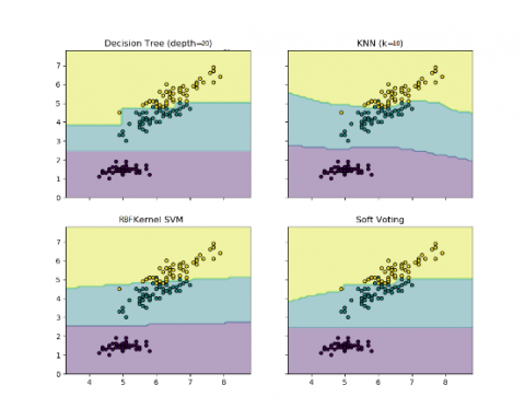
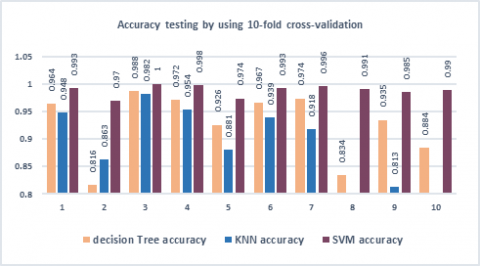
The comparison made between three algorithms: SVM, K-NN, and Decision Tree, in Figure 10 the SVM algorithm has proposed this dissertation since based on the literature, SVM has a reputation for giving high accuracy for traffic sign recognition. The results showed that SVM achieved higher accuracy for all value of k-fold splits. The highest accuracy is obtained at k=3 with 100% accuracy while the KNN and Decision Tree got 98.2% and 98.8% respectively.
Figure 10. The accuracy comparison between SVM, KNN, and DTs
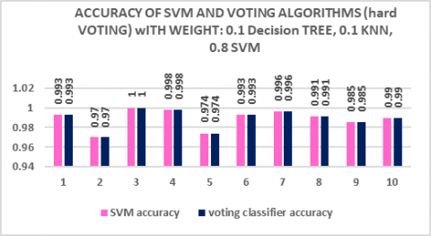
3.1 Accuracy results for voting algorithm (Hard voting)
Figure 11 depicts the results when the voting classifier uses hard voting, which depends on selecting a model from an ensemble to determine the final prediction with a straightforward majority vote for precision. The candidate classifier selected by hard voting depends on the highest weight given. The comparison between SVM and voting classifier shown in the Figure 11. In the 10-fold cross-validation, the SVM got higher accuracy to compare with KNN and DTs; it obtained the majority voting, which means that the voting classifier chooses the SVM accuracy values.
Figure 11. The accuracy comparison between SVM and voting classifier with the hard voting aggregation method
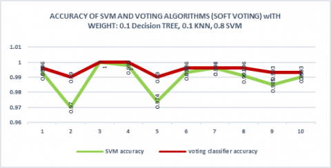
3.2 Accuracy results for voting algorithm (Soft voting)
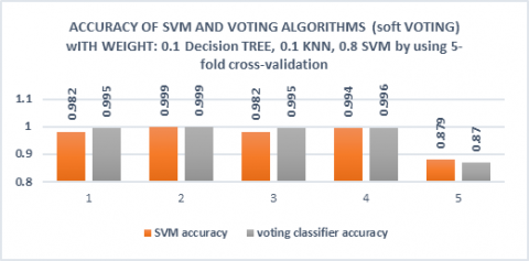
In this experiment, the voting classifier uses soft voting, which uses the classifier's predicted probabilities (p) to predict the class labels. The results of the voting classifier by using soft voting depend on the weight given to each of the base classifiers. First, the weights are assigned as follows. The Decision Tree set to 0.1, K-NN set 0.1 and SVM was 0.8. Figure 12 shows comparison between SVM and voting classifiers based on accuracy. From the results, voting classifier obtained greater accuracy in nine of ten folds. Both SVM and voting classifiers achieved 100% accuracy at fold 3. Further, the voting classifier obtained 100% at fold 4.
Figure 12. Accuracy comparison between SVM and Voting classifier (soft voting) when weight (0.1, 0.1, 0.8)
A high level of accuracy compares SVM and voting classifier. In this figure, nine out of 10 instances, the voting classification has achieved higher accuracy. More so, SVM and voting classifier nevertheless accomplished 100% accuracy when K=3. In regards, when the K=4, the voting classification obtained 100 percent.
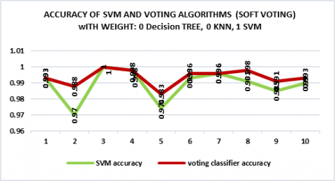
Figure 13. Accuracy comparison between SVM and Voting classifier (soft voting) when weight (0, 0, 1)
The voting classification used in the simulation based on the combination of three support vector machines, K-Nearest neighbour, and Decision Tree algorithms. It can see from Figure 13 the classification has been given more accuracy in nine out of ten cases. The comparison between SVM and voting classifiers based on high accuracy. However, when K=3, SVM and voting classification attained 100% accuracy. Also, when the K=4 the voting classifier and SVM achieved same 99.8%. Furthermore, 0 for DTs, 0 for KNN, and 1 for SVM were used in Figure 13.
The experimental in this figure shows a comparison between the SVM and voting classifier; the voting classifier depends on ensemble three algorithm which are SVM, KNN, and Decision Tree. Voting classifiers obtained high accuracy in nine out of tenth cases. However, SVM and voting classifiers achieved 100% accuracy when K=3. Further the voting classifier got 100% when the K=4. Moreover, the weight used in table, was 0.2 for DTs, was 0.2 for KNN, and 0.6 for SVM. The weight used in this experiment gives better results than other experimental.
From Figure 14, it can see that voting classifier used in the simulation which depends on the combination of three algorithms that support vector machine, K-Nearest algorithm, and Decision Tree algorithm that splits data into five k-fold. In Figure 14, voting classifier obtained greater accuracy in three out of five cases than SVM. Also, the SVM achieved 0.009 higher than voting classifier when K=5. Further the voting classifier and SVM got 0.999 % when the K=2. Moreover, the weight used in table 0.1 for DTs, is 0.1 for KNN, and 0.8 for SVM.
Figure 14. The comparison between SVM, Voting classifier
Table 3 illustrates the comparison of PC with the real time Raspberry Pi’s execution timing which demonstrate the Raspberry Pi's processing limitations for real-time traffic sign recognition, especially in situations requiring quick decisions due to dynamic or fast driving. Despite the system's high classification accuracy, it achieves the lowest execution time compared to its counterpart, making it suitable for static sign recognition but not for high-speed scenarios.
Table 3. Time comparison of Chinese traffic sign recognition on PC and Rasperry Pi
|
Classifier |
On PC |
On Raspberry Pi |
|
Decision Tree |
42.044s |
426.48s |
|
K-NN |
42.044s |
426.8s |
|
SVM |
612.47s |
2831.88s |
|
Voting |
657.12s |
3139.08s |
Traffic Sign Recognition (TSR) systems are crucial in intelligent transportation systems (ITS) to address the issue of the continuous traffic sign rise and accidents. The approach involves converting images from RGB to grayscale, extracting feature histograms for edge detection, and using support vector machine (SVM) for image recognition. The SVM classifier achieves the highest accuracy compared to KNN and DTs algorithms, with the highest accuracy achieved when the k-fold equals three. Soft voting classifiers also achieve the highest accuracy. The best accuracy was achieved using a weighted ensemble where weights were assigned proportionally to each classifier’s standalone accuracy on the validation set, with Decision Trees receiving the highest weight (0.8), and Decision Trees and K-NN each assigned 0.1. Hard voting results in lower accuracy than soft voting. Raspberry Pi is chosen due to its small size, lightweight, low power consumption, and flexibility in development. It is more convenient than PC-based traffic sign recognition schemes in smart cars due to its open source code and free software development on Linux. The experimental results indicate that Raspberry Pi boards are an efficient technique based on the achieved results.
[1] Hussain, S., Abualkibash, M., Tout, S. (2018). A survey of traffic sign recognition systems based on convolutional neural networks. In 2018 IEEE International Conference on Electro/Information Technology (EIT), Rochester, MI, USA, pp. 570-573. https://doi.org/10.1109/EIT.2018.8500182
[2] Chakravorty, P., Das, A.B. (2024). Advances in high moisture extrusion cooking for meat analogue with 3D and 4D printing approaches: A comprehensive review. Discover Food, 4: 137. https://doi.org/10.1007/s44187-024-00222-4
[3] An, F.P., Wang, J.R., Liu, R.J. (2024). Road traffic sign recognition algorithm based on cascade attention-modulation fusion mechanism. IEEE Transactions on Intelligent Transportation Systems, 25(11): 17841-17851. https://doi.org/10.1109/TITS.2024.3439699
[4] Boukerche, A., Hou, Z.J. (2021). Object detection using deep learning methods in traffic scenarios. ACM Computing Surveys (CSUR), 54(2): 1-35. https://doi.org/10.1145/3434398
[5] Lim, X.R., Lee, C.P., Lim, K.M., Ong, T.S. (2023). Enhanced traffic sign recognition with ensemble learning. Journal of Sensor and Actuator Networks, 12(2): 33. https://doi.org/10.3390/jsan12020033
[6] Fredianelli, L., Carpita, S., Bernardini, M., Del Pizzo, L. G., Brocchi, F., Bianco, F., Licitra, G. (2022). Traffic flow detection using camera images and machine learning methods in ITS for noise map and action plan optimization. Sensors, 22(5): 1929. https://doi.org/10.3390/s22051929
[7] Müller, A., Österlund, H., Marsalek, J., Viklander, M. (2020). The pollution conveyed by urban runoff: A review of sources. Science of the total environment, 709: 136125. https://doi.org/10.1016/j.scitotenv.2019.136125
[8] Cervantes, J., Garcia-Lamont, F., Rodríguez-Mazahua, L., Lopez, A. (2020). A comprehensive survey on support vector machine classification: Applications, challenges and trends. Neurocomputing, 408: 189-215. https://doi.org/10.1016/j.neucom.2019.10.118
[9] Liu, Z.W., Qi, M.Y., Shen, C., Fang, Y., Zhao, X.M. (2021). Cascade saccade machine learning network with hierarchical classes for traffic sign detection. Sustainable Cities and Society, 67: 102700. https://doi.org/10.1016/j.scs.2020.102700
[10] Masud Rana, M., Ahmed, K. (2019). Feature selection and biomedical signal classification using minimum redundancy maximum relevance and artificial neural network. In Proceedings of International Joint Conference on Computational Intelligence: IJCCI 2018, pp. 207-214. https://doi.org/10.1007/978-981-13-7564-4_18
[11] Eitel, A., Springenberg, J.T., Spinello, L., Riedmiller, M., Burgard, W. (2015). Multimodal deep learning for robust RGB-D object recognition. In 2015 IEEE/RSJ International Conference on Intelligent Robots and Systems (IROS), Hamburg, Germany, pp. 681-687. https://doi.org/10.1109/IROS.2015.7353446
[12] Mienye, I.D., Jere, N. (2024). A survey of decision trees: Concepts, algorithms, and applications. IEEE Access, 12: 86716-86727. https://doi.org/10.1109/ACCESS.2024.3416838
[13] Song, S.Q., Ye, X.F., Manoharan, S. (2025). E-MobileViT: A lightweight model for traffic sign recognition. Industrial Artificial Intelligence, 3(1): 3. https://doi.org/10.1007/s44244-025-00024-2
[14] Cavagnero, N., Rosi, G., Cuttano, C., Pistilli, F., Ciccone, M., Averta, G., Cermelli, F. (2024). PEM: Prototype-based efficient maskformer for image segmentation. In Proceedings of the IEEE/CVF Conference on Computer Vision and Pattern Recognition, pp. 15804-15813.
[15] Jia, J., Kang, J., Chen, L., Gao, X., Zhang, B., Yang, G. (2025). A comprehensive evaluation of monocular depth estimation methods in low-altitude forest environment. Remote Sensing, 17(4): 717. https://doi.org/10.3390/rs17040717
[16] Pan, X., Zhang, Z.J., Liu, Y.Z,, Yang, C.C., Chen, Q.F., Cheng, L., Lin, J.X., Chen, R.Q. (2019). Graph-based rgb-d image segmentation using color-directional-region merging. In ICASSP 2019 - 2019 IEEE International Conference on Acoustics, Speech and Signal Processing (ICASSP), Brighton, UK, pp. 2417-2421. https://doi.org/10.1109/ICASSP.2019.8682701
[17] Khalid, S., Muhammad, N., Sharif, M. (2019). Automatic measurement of the traffic sign with digital segmentation and recognition. IET Intelligent Transport Systems, 13(2): 269-279. https://doi.org/10.1049/iet-its.2018.5223
[18] LeCun, Y., Jackel, L., Bottou, L., Brunot, A., et al. (1995). Comparison of learning algorithms for handwritten digit recognition. In International Conference on Artificial Neural Networks, 60(1): 53-60.
[19] Breiman, L., Friedman, J., Olshen, R.A., Stone, C.J. (1984). Classification and Regression Trees. Chapman and Hall/CRC.
[20] Zadeh, A., Nosoudi, N., Halley, R., Kiani, C., Ramirez-Vick, J.E. (2025). Predictive analytics for de novo malignancies after lung transplantation. Intelligent Decision Technologies, 19(2): 1040-1053. https://doi.org/10.1177/18724981241296492